Abstract
The significant increase in non-performing loans (NPLs) during the escalating recession of the Greek economy motivates us to study the predictive power of credit rating models in periods of economic shocks. In parallel, we examined the responsibilities of bank management in the expansion of NPLs in this adverse environment. Certain studies connect bad loans with turbulent conditions. Our paper weighs the relative significance of both economic shock and management effectiveness using data at an individual level, which provides the originality of our study. We use a unique dataset of small business loans that were granted during 2005 (expansion period) by a large commercial Greek bank, and we explore their performance between 2010 and 2012 (early recession period). In the context of a stepwise methodology, we compare the Bank’s credit scoring model with three other prediction models (binomial logistic regression, decision tree, and multilayer perceptron neural network) to check both the predictive ability of credit scoring models during recession and the effectiveness of bank management. The comparative analysis confirms the management’s responsibilities in granting NPLs, since the Bank’s model exhibited the worst predictive performance. Additionally, we find that adverse external conditions lead to an increase in NPLs and decrease the predictive performance of all credit scoring models. The study offers a reliable methodological tool for lending management in economic downturns.
1. Introduction
Micro and small enterprises (MSEs) represent up to 99% of all businesses operating in the European Union. Moreover, they are strongly dependent on the banking system since 75–80% of all enterprises are bank-financed, especially with short-term bank loans. (European Banking Authority [EBA], 2016). MSEs’ credit risk seems to be high since their financial reporting quality is lower and the asymmetric information is higher than those of other businesses (Duarte et al., 2016). After the financial crisis of 2008, the level of non-performing loans (NPLs) for MSEs was the highest in most EU countries (18.5%, European Banking Authority [EBA], 2016), proving that they are more vulnerable to adverse economic conditions than other enterprise groups. According to Christodoulou-Volos (2025), lower economic growth, higher inflation, and higher interest rates correlate with an increase in non-performing loans (NPLs). Moreover, economic policy uncertainty, unemployment, capital adequacy, and liquidity risk during recession periods affect NPLs (Papadamou & Pitsilkas, 2025). Maztoul (2025) studied a dataset of 131 OECD commercial banks for 10 years. The empirical findings provide strong evidence that banks’ financial performance is negatively affected by non-performing loans (NPLs) and that institutions with higher ESG (Environmental, Social, and Governance) scores tend to have lower NPL ratios. The study concludes that enhancing sustainability practices contributes to improved financial performance by mitigating credit risk. Integrating sustainability into banking operations strengthens risk management, which in turn supports financial outcomes. Moreover, the results highlight that the Social and Governance components play a significant role in this relationship, while the Environmental component has a more ambiguous impact. These findings underscore the importance for banks to improve their ESG performance due to its positive influence on loan quality and overall financial health.
Accurately modeling NPLs is critically important for a wide range of stakeholders seeking to assess bank performance, including shareholders, bank managers, competitors, regulators, and credit rating agencies (Karagiannis & Kourtzidis, 2025).
In this paper, we focus on the evaluation process of bank financing, as we believe that the management of NPLs is crucial for financial stability, especially during recession periods. In this direction, we try to find out if the remarkable increase in NPLs is a result of poor bank managerial ability in risk-taking behavior (Andreou et al., 2016) or the country’s adverse macroeconomic conditions. When bank managers apply poor credit scoring models or ignore the model rating to increase the number of loans granted and their market share during expansion periods, they then expect a greater increase in NPLs in periods of recession. On the other hand, we also argue that during economic downturns, the level of NPLs could mark a significant increase that strongly challenges management decisions. Manz (2019) presented a literature review of 44 studies on determinants of NPLs published for the period 1987 to 2017 in 30 peer-reviewed journals. The paper concluded that the interaction of loan- and asset-specific events with macroeconomic and bank-specific factors remains poorly understood and deserves additional empirical research.
Although there is some literature on poor bank managerial ability (Berger & DeYoung, 1997; Williams, 2004; Louzis et al., 2012; Belaid et al., 2017), this does not evaluate lending management during recessionary periods. In such periods, credit risk materializes and raises concerns for a further increase in the NPL ratio. In this way, external environmental deterioration fully reveals bad management decisions that are taken more easily in the growth period (in which loan demand booms), resulting in a continuously decreasing performance of marginally efficient loans. Although specific studies connect bad loans with turbulent conditions (Quagliariello, 2007; Konstantakis et al., 2016), to the best of our knowledge, no study weighs the relative significance of both dimensions of NPLs, systematically considering adverse external effects and using data at an individual level, providing our study’s originality.
In our paper, we compare the Bank’s credit scoring model with three other prediction models that the literature proposes, such as binomial logistic regression, decision tree, and multilayer perceptron neural network, to answer our research questions. The comparative analysis confirms the management’s responsibilities in granting NPLs, since the Bank’s model exhibited the worst predictive performance. Additionally, we find that adverse external conditions lead to an increase in NPLs and decrease the accuracy of all empirical methods used in the study.
The Greek economy is a bank-based system, similar to other European countries, such as Spain, Portugal, Italy, etc. (Duarte et al., 2016). So, the study of the responsibilities of banking management in the significant increase in NPLs during the recession is a typical case study that can lead to general conclusions. Although the EU average NPL ratio was up to 6% in September 2015, the NPL ratio in Greece was extremely high (43.5%), which is the second-highest NPL ratio in Europe after the NPL ratio of 50% in Cyprus (European Banking Authority [EBA], 2016). In our paper, we examine whether the increase in NPLs from August 2010 to July 2012 is due to bad management during the expansion period or is a matter of the escalating recession of the economy.
The Greek retail banking system is oligopolistic, consisting of four systemic institutions that provide similar services and products and have a similar structure in terms of retail network and organizational form. The data was collected manually and consists of 3.294 loans to small businesses that were granted in 2005, a year during which the Greek economy was in a phase of redefinition after the 2004 Olympic Games. We explore the performance of small business loans from August 2010 to July 2012 (early recession period of the Greek economy). During the recession period, all systemic Greek banks were under the supervision of the European Central Bank (ECB) and the Bank of Greece. Accordingly, the high homogeneity of the Greek systemic banks gives our results high representativeness for the entire Greek banking sector.
Our paper contributes to the existing literature related to NPLs’ determinants (Louzis et al., 2012) and the literature of credit scoring models (Crook et al., 2007; Louzada et al., 2012) in diverse ways. First, this offers a reliable response to whether bad loan performance is the result of bad management or caused by an adverse external environment. In particular, the findings confirm the bad management hypothesis and demonstrate that poor decision-making is very vulnerable to economic fluctuations. Moreover, we observe that loans that were 90 days past due in the first year indicated a further deterioration in the second year. As an important implication, it seems to be an urgent focus for banks to avoid loans becoming more than 90 days past due. Secondly, the paper considers, for the first time, a relatively large number of micro and small-sized borrowers’ idiosyncratic features, thus substantially differing from the current literature (e.g., Louzis et al., 2012; Anastasiou et al., 2016) that emphasizes both macroeconomic factors and bank-specific characteristics for NPLs accumulation at the aggregated level. Moreover, the paper assesses the relative accuracy of several credit scoring models using data from emerging economies (Abdou et al., 2007; Louzada et al., 2012; Mileris & Boguslauskas, 2011), where banks’ credit scoring models record the worst accuracy compared to the models proposed in the literature. In this paper, we use three credit scoring models widely used in the literature, and we focus on the efficiency and the evolution of all credit scoring models over time to answer the bad management and bad luck hypotheses.
The rest of the paper is structured as follows. In Section 2, we present a literature review of bad management and credit scoring models. In Section 3, we provide the dataset and its descriptive statistics. In Section 4, we set the research methodology, and we provide a short presentation of the different credit scoring models. In Section 5, we present our main results. In Section 6, we discuss the main findings of our study and we conclude the paper.
2. Literature Review
2.1. Bad Management Hypothesis
According to the bad management hypothesis, introduced by Berger and DeYoung (1997), poor management skills in the underwriting process (credit scoring models), appraisal of pledged collaterals, and monitoring borrowers are associated with increases in future problem loans. Under these circumstances, “bad managers” follow a liberal credit policy to boost current earnings, increase market shares, and, in conjunction with the income smoothing activities by borrowers in expansionary phases, they conduct inadequate credit risk loan assessment. There are some studies on the bad management hypothesis at the aggregate level (Berger & DeYoung, 1997; Partovi & Matousek, 2019; Louzis et al., 2012; Williams, 2004) that provide interesting findings but ignore the substantial impact of crisis effects on bank lending decision-making.
Exogenous crisis effects can challenge bad management decisions further. In this framework, certain studies examine bad loans under turbulent conditions (Quagliariello, 2007; Konstantakis et al., 2016; Makri et al., 2014; Tmava & Spahiu, 2025; Undji & Sheefeni, 2025); however, they do not consider strategic firm-specific considerations, Bank lending managerial options, and micro-level data. Akuoko-Kanadu and Mahmud (2025) applied the Arellano–Bond Generalized Method of Moments dynamic panel estimation technique to a sample of 493 banks across 31 Sub-Saharan African (SSA) countries between 2011 and 2019. Their findings indicate that corruption and economic growth have had significant, but opposite, effects on NPLs in the region—corruption exerting a positive influence and economic development a negative one. In a turbulent environment, commercial banks face increased credit risk due to the reduced cash flows of their business borrowers. At the same time, household borrowers receive lower income payments because of wage cuts or unemployment. In this high-risk environment, the rise in problem loans and the decline in collateral values lead to a significant tightening of credit conditions, as banks become increasingly unwilling to provide new credit. Thus, Berger and DeYoung (1997) suggest that external events cause an increase in problem loans for the Bank, and consequently, a decrease in performance. The specific hypothesis suggests a circular relationship between the macroeconomic environment and loan quality, implying that in expansion years, borrowers’ incomes improve, and thus their capacity to repay their loans increases. In turn, when the economy enters a recessionary phase, NPLs augment as unemployment rises, disposable income declines, and borrowers face difficulties in repaying their debt obligations.
2.2. Credit Scoring Techniques
The global financial crisis of 2008 has focused the attention of financial institutions on the control and management of credit risk. A good credit risk assessment method can help financial institutions lend to trusted borrowers, thereby increasing their profits, and refuse lending to unreliable borrowers, thereby reducing losses. The precision of the credit rating model of prospective borrowers is critical for the profitability of financial institutions (Wang et al., 2012). Even a 1% improvement in the accuracy of recognizing bad borrowers leads to a significant reduction in losses for financial institutions (Hand & Henley, 1997). The accuracy of scoring models is crucial for banks’ profitability, as credit management needs to identify potential bad clients and minimize the chance of default (Lee et al., 2002). Researchers developed several credit scoring models that could be categorized into two main techniques. In the first category, there are the statistical credit scoring models, such as Linear Discriminant Analysis (Altman & Saunders, 1998), Logistic Regression Analysis (Lee et al., 2002; Gordy, 2000), and Multivariate Adaptive Regression Splines (Friedman, 1991). The most popular technique, logistic regression, allows for the best accuracy (Louzada et al., 2012). In the second category, there are the neural network machine learning models, such as Artificial Neural Networks (Zopounidis & Doumpos, 2002), Decision Trees (Dilsha & Kiruthika, 2014), Case-Based Reasoning (Shin & Han, 2001), and Support Vector Machines (Trustorff et al., 2011). Many researchers claim that the artificial intelligence models are more accurate than the statistical credit scoring models since the relationship between variables is non-linear (Lee et al., 2002).
To measure the predicted performance of a credit scoring model, we could use both statistical (average accuracy, precision, specificity, etc.) and information measures (entropy, etc.). In general, researchers choose the credit scoring models according to the dataset, the independent variables, and the purpose of the classification (Twala, 2010). On the other hand, Sun and Vasarhelyi (2018) developed a deep neural network to evaluate the risk of credit card delinquency based on the client’s characteristics and spending behaviors using a dataset of 711,397 credit card holders from a large bank in Brazil. Compared with machine-learning algorithms of logistic regression, naive Bayes, traditional artificial neural networks, and decision trees, they found that the proposed deep neural networks have a better overall predictive performance with the highest F scores and area under the receiver operating characteristic curve.
In many cases, banks are developing their credit scoring models to evaluate the probability of default of potential borrowers. Studying the literature, we found that in most cases, the models used by the banks performed worse than the models suggested by the relevant literature. Louzada et al. (2012) compared the performance of the model applied by a Brazilian bank with different scoring models, and they showed that the Bank’s model performed worst. Mileris and Boguslauskas (2011) suggested that the credit scoring they used had better accuracy than the Lithuanian Bank’s scoring model. Similarly, Abdou et al. (2007) found that the credit scoring model which an Egyptian bank uses scored the lowest accuracy compared to logistic regression and discriminant analysis models.
In our paper, we compare the Bank’s credit scoring model with three other credit scoring techniques (i.e., Logistic Regression, Decision Tree, and Multilayer Perceptron Neural Networks) and we examine their behavior during the worsening recession of the Greek economy.
3. The Evolution of the Greek Economy
Greece’s entrance into the Eurozone in 2002 and the Olympic Games of 2004 led the Greek economy to remarkable growth in the first years of the millennium. During this period, Greek banks pursued an expansionary policy in the field of private sector lending and participation in the financing of public debt. Greek banks also implemented an aggressive lending policy to households and MSEs because of intense competition. However, the global financial crisis and, most importantly, the structural problems of the Greek economy led to a prolonged recession period from September 2008 (Aggelopoulos & Georgopoulos, 2015).
As shown in Table 1, the GDP growth stalled after the Olympic Games of 2004, but during 2006 and 2007, the Greek economy recorded remarkable growth. The GDP declined for the first time in 2008 by 0.3% (after fifteen years of continuous growth). In 2011, the reduction of GDP rose to −9.1%, but after the restructuring of sovereign debt in 2012 (Private Sector Involvement), the reduction of GRD was limited to −3.2%. The gross debt as a percentage of GDP increased from 103.1% in 2007 to 172.1% in 2011 and reached 177.7% in 2013, despite the sovereign debt’s restructuring. At the same time, private debt as a percentage of GDP increased from 114.6% in 2007 to 144.4% in 2011 and 147.8% in 2013. As a result, the creditworthiness of the Greek economy in October 2009 was downgraded, and the yield spread between Greek and German bonds was significantly widening. Given the deteriorating financial condition of the Greek economy, the percentage of NPLs dramatically increased, since both households and enterprises were unable to pay their loan obligations. The percentage of non-performing business loans of Greek banks increased significantly after the outbreak of the financial crisis (in September 2008), while there was a significant further increase from 2010 onwards. At the end of 2013, the NPL ratio had increased dramatically to 39.5%. Generally, the restructuring of NPLs is a significant concern for the ECB and EBA.

Table 1.
Statistics of the Greek economy and the NPL ratio of the Greek banking sector over the period 2003 to 2013.
4. Research Methodology
In our paper, we set the loans’ performance as the dependent variable at three time points. We observe the performance of loans in August 2010, August 2011, and July 2012. Thereafter, to control the effectiveness of bank management, we check the accuracy of the Bank’s model compared with the performance of three other models (Binomial Logistic Regression, Decision Tree, and Multilayer Perceptron Neural Network). Furthermore, to check the bad luck hypothesis, we observe the evolution of the predicting ability of all models during the escalating recession of the Greek economy.
4.1. Loan Characteristics and Borrowers’ Features
Loan characteristics and borrower’s features were determined as independent variables to demonstrate a credit scorecard and measure the probability of default of business loans. Particularly, we use qualitative information (such as bank relationship, residence status, etc.) to predict the credit risk of an MSE (Gupta et al., 2015). The independent variables are justified by the “Five Cs of Credit” (DeVaney & Lytton, 1995), which represent five general borrower’s characteristics, trying to estimate the probability of default (Character of the borrower, Capital, Collateral, Capacity, and Economic Conditions). In our analysis, we use ten independent variables that were used in the Bank’s model (borrowers’ idiosyncratic). To make the results of the models comparable with the scorecard applied by the Bank at the time the loans were granted, macroeconomic factors have not been added as independent variables in our research. The definition of each variable is summarized in Table 2.
Table 2.
Loan characteristics and borrowers’ features.
4.2. Logistic Regression
According to Siddiqi (2006), logistic regression is a common technique used to develop scorecards in most financial industry applications where the predicted variable is categorical. In cases where the predicted variable is binary (good/bad), multiple logistic regression is used. Logistic regression uses a set of predictor characteristics to predict the probability of a specific outcome. The equation for the logit transformation of the probability of an event is shown by the following:
where
- p = posterior probability of “event”, given inputs;
- xi = independent variables;
- β0 = intercept of the regression line;
- βk = parameters.
Logit transformation is the log of the odds, that is, log(p(event)/p(non-event)), and is used to linearize posterior probability and limit the outcome of estimated probabilities in the model to between 0 and 1. Maximum likelihood is used to estimate parameters β1 to βk. These parameter estimates measure the rate of change of logit for a one-unit change in the independent variable (adjusted for the other inputs), that is, they are the slopes of the regression line between the target and their respective independent variables x1i to xki.
In our paper, we use as independent variables the loan characteristics and the borrowers’ features that are presented in Table 2. Appendix A presents the coefficients of the binary logistic regressions we used. So, the logistic regression of our model is formulated as follows:
where
- Yi = A dummy variable taking the value 1 if a loan is non-performing or the value 0 if the loan is performing;
- BH = Firm’s owner’s bad trading past;
- Ag = Age of the firm’s owner;
- BR = Relationship between the firm’s owner and the Bank;
- Co = Type of collateral;
- LTT = Loan to turnover ratio;
- OF = Own facilities;
- P = Mortgage-free property;
- R = Residence status;
- LT = Loan type;
- Yr = Years of operation;
- β0 = Intercept of the regression line;
- βk = Parameters.
4.3. Classification and Regression Trees
The term “classification” refers to the act of assigning an object to one of the predefined classes within a set of classes. Each object in a dataset has several attributes (X1, …, Xk), where Π(Χi) is the domain of attribute Xi. In addition, each object has an attribute C, which denotes the class to which it belongs, with Π(C) symbolizing the domain of the attribute of class C. The categorization involves finding a function f: Π(X1) x… x Π(Xk) → Π(C), which is called the classification model. If we know the values of the attributes X1, …, Xk of an object, but not the value of the attribute C, then we apply a categorization model and assign the object to the class f(X1, …, Xk). A decision tree is one of the most popular classification models (Figure 1).
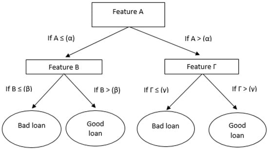
Figure 1.
A decision tree case.
The decision tree is a graph with the classic tree structure, where we distinguish the following: (a) an initial or decision node, which is the root, (b) the inner nodes, which are the edges or branches, and (c) the outer nodes, which are the leaves. At each node (inner or outer) outside the root, a directed edge enters from another node. Each inner node corresponds to a feature used to separate the tree further. At the edges coming out of the root or any inner node, there is a control condition based on the separator characteristic. The process of constructing a decision tree is iterative. It can be briefly described as follows: First, we select an attribute, which refers to the root of the tree, and then construct an edge and a node for each of the distinct values of the attribute. These two steps are repeated continuously until all the attributes are inserted into the nodes of the tree. In the literature, we found different algorithms that were used for constructing a decision tree (ID3. C5.0, and CART (Quinlan, 1986)). The classification and regression trees (CART models) are a classification method that has been used successfully in credit scoring (Zopounidis & Doumpos, 2002).
In our paper, we use a CART model. Appendix C presents the information on our CART models. As “initial or decision” nodes, we set the loan characteristics, the categories of each characteristic are defined as “edges” or “branches,” and as “leaves,” we set the performance of each loan (performing or non-performing). We finally chose the minimum number of loan characteristics that maximizes the average accuracy and minimizes the estimated misclassification cost.
4.4. Multilayer Perceptron Neural Network
A multilayer perceptron neural network consists of a set of input nodes that make up the input layer, one or more hidden layers made up of computing neurons, and an output layer also made up of computing neurons (Figure 2). The input signal (input standard) moves through the network forward, i.e., from one level to the next. Multilayer perceptron neural networks are usually trained with supervised learning rules. An algorithm that is very often used for this purpose is known as the Back-Propagation algorithm and is based on the rule of learning with error correction.
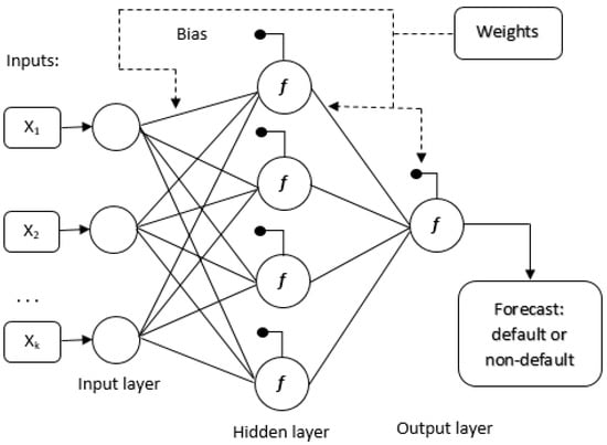
Figure 2.
Artificial neural network—multilayer perceptron.
Two types of signals are transmitted in the network: (1) Function signals. A function signal is an input signal (stimulus) that starts at the input nodes of the network, propagates forward, from neuron to neuron, and ends at the output neurons of the network. In each neuron of the network through which the signal passes, it is calculated as a function of all the incoming signals and the corresponding weights of the synapses that end up in that particular neuron. (2) Error signals. An error signal starts at the output neurons of the network and propagates backwards from level to level. In each neuron, this signal is calculated from an error-dependent function.
Each neuron, in the input layer (i = 1, …, n), yields the value of an estimator of the vector x. Each neuron in the hidden layer (j = 1, …, q) produces the so-called activation
Neurons in the output layer (k = 1, …, m) behave like the neurons in the hidden layer to produce the network output result:
where wij and wjk are weights.
The logarithmic function:
or the alternative tangent hyperbolic function:
are commonly used in the upper output of the network for the functions f and g. The logarithmic function is appropriate to the output layer if we have a binary classification problem, as in credit scoring, so that the output can be considered a default probability. The structure of a neural network with a single hidden layer is capable of approximating any continuous, bounded, and integrable function.
Appendix B presents the information on the Multilayer Perceptron Neural Networks we used. Our model is as follows:
where
- Yi = A dummy variable taking the value 1 if a loan is non-performing or the value 0 if the loan is performing;
- BH = Firm’s owner’s bad trading past;
- Ag = Age of the firm’s owner;
- BR = Relationship between the firm’s owner and the Bank;
- Co = Type of collateral;
- LTT = Loan to turnover ratio;
- OF = Own facilities;
- P = Mortgage-free property;
- R = Residence status;
- LT = Loan type;
- Yr = Years of operation;
- wij and wjk are weights.
4.5. The Dataset
The dataset contains loans that were granted to micro and small enterprises (MSEs—EU definitions for SMEs define a firm as micro if it has less than 10 employees and an annual turnover of less than 10 million and as small if it has less than 50 employees with an annual turnover of less than 10 million). The loans’ features and borrowers’ characteristics are collected manually from the Bank’s Management Information System (MIS). The final dataset contained 3294 loans of Greek MSEs that were granted during 2005 (expansion period). We study their performance from August 2010 to July 2012, two years after the onset of the financial crisis and the bankruptcy of Lehman Brothers Holdings Inc. (September 2008). During this period, Greek banks implemented two re-capitalizations to avoid collapse.
To obtain a loan, the prospective borrower fills in their details in an application. In particular, this provides information on the financial situation of the company, its primary demographic characteristics, and its loan and deposit cooperation with the Bank. The applications are registered in the credit scoring model of the Bank by a Small Business officer and receive an evaluation: “Approve”, “Referral”, and “Reject”. Then, the credit director decides whether or not to approve the loan, taking into account the SB officer’s suggestion and the Bank’s guidelines. Therefore, the final financing decision is based on the subjective judgment of credit directors, beyond the categorization of the credit scoring model.
Table 3 shows the evolution of NPLs by rating category based on the Bank’s scorecard. We mention that loans, although rejected by the scorecard of the examined Bank, were granted, with the worst performance throughout the studied period; following loans that were designated as ‘Referral’, while ‘Approve’ loans noted smaller percentages of NPLs. The percentage of non-performing loans that were classified as “Reject” was very high from August 2010 (23.92%) and increased dramatically to 42.11% in July 2012. However, the recession affected all types of loans as well. The percentage of non-performing “Approve” loans increased from 4.58% in August 2010 to 21.15% in July 2012. Moreover, deep recession (and the respective rise of NPLs) significantly deteriorated the predictive power of all credit scoring models, thus further weakening the effectiveness of such lending evaluation tools, considerably challenging bank management.
Table 3.
Non-performing loans per decision of the Bank’s credit scoring model.
The descriptive statistics are presented in Table 4. The loan’s performance was determined as the dependent variable. Specifically, a loan is classified as non-performing when the delay exceeds 90 days, according to the basic rules of Basel II. In the literature, the behavior of loans is controlled both in a particular month and during a period, usually 12 months (Makri et al., 2014; Louzis et al., 2012). We control the loans’ behavior for three months during two years (August 2010, August 2011, and September 2012). The percentage of NPLs rose from 7.7% in August 2010 to 27% in September 2012.
Table 4.
Structure of the dataset (3294 total loans).
As regards the loan type, the dataset consists of 275 loan applications for business equipment, 428 loan applications for business property, 1884 applications for credit lines and overdrafts, and finally 707 applications related to fixed-term working capital loans. Moreover, 43.3% of the loans are unsecured and 56.7% are covered. Regarding the occurrence of existing cooperation with the Bank, 71.9% of borrowers had a previous relationship with the Bank, while 28.1% were new customers. Also, 41% of the loans were granted to businesses operating up to 5 years in the same field, while the remaining 59% were granted to businesses operating for more than 5 years.
Moreover, 49.6% of businesses had their own facilities, and only 9.3% of the business owners experienced a bad trading past. A total of 82.4% of the borrowers and the guarantors had mortgage-free property; 68.1% of the borrowers lived in their home, 17.9% lived with their parents, and only 14% lived in a rental home.
The mean years of operation of the businesses was 10.3 years, and the mean age of the businesses’ owners was 42.55 years. Finally, regarding the loan-to-turnover ratio, the mean LTT was 31.9% with a standard deviation of 0.640.
Figure 3 shows the evolution of loan arrears between the first period (08/2010–07/2011) and the second period (08/2011–07/2021). In particular, we study the maximum days of delay (bucket) that each loan showed during the first and second period. Firstly, we can see that 88% of loans that were more than 90 days late during the first period are still more than 90 days late during the second period. On the other hand, only 67% of the loans without delays during the first period remain up-to-date (no delays) during the second period, while the remaining 33% show some delays. At the same time, 52% of the loans that showed a delay of up to 30 days in the first period showed a deterioration in the second period, and 23% showed a delay of more than 90 days. The percentage of loans with a delay of more than 90 days during the second period increases further when we study the loans with a maximum delay of up to 60 and 90 days, respectively, during the first period. A total of 51% of loans with a maximum delay of up to 60 days and 59% of loans with a maximum delay of up to 90 days during the first period showed a delay of more than 90 days during the second period. We therefore observe that avoiding the transfer of a loan at a delay level of more than 30 days is critical to avoid the increased possibility of a loan being classified as non-performing (bucket 90+) within the next 12 months.
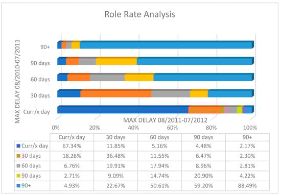
Figure 3.
Temporal scaling NPLs per bucket for the 3294 loans between the first and the second year of the studied period. Notes: Figure 3 presents an analysis of delays according to the days a loan is overdue. The vertical axis measures the number of days of overdue debt during the first period (August 2010 to July 2011). The horizontal axis measures the number of days of overdue loans during the second period (August 2011 to July 2012). The longer the delay of a loan during the first twelve-month period, the greater the possibility of displaying the same or more days of delay in the second 12-month period.
5. Results
Table 5 presents the correlations between the independent variables. Specifically, the Pearson correlations appear on the lower diagonal and the Spearman correlations appear on the upper diagonal. We observe that most observations are statistically significant at the 1% or 5% level. At the same time, we observe that the correlations range at levels lower than 0.5, indicating low to moderate correlations between the independent variables. Therefore, there is no issue of multicollinearity.
Table 5.
Pearson and Spearman correlation matrix.
To ensure the robustness of the models and eliminate the risk of overfitting of the three proposed models, we proceeded to separate the sample into a training sample (approximately 70% of the cases) and a test sample (approximately 30% of the cases). We then compared the efficiency of the models between the two subsamples. As we observe in Table 6, the differences between the training sample and the control sample are less than 2% for all models. Therefore, the reliability and robustness of the models are ensured. We then proceeded to calculate the metrics Average Accuracy, F1, and Estimated Misclassification Cost of the models, using the results of the test sample and comparing them with the Bank’s credit rating model.
Table 6.
Cross-validation results on predictive performance.
The comparative analysis is presented in Table 7. To compare the predictive performance of the credit scoring models studied, we calculate the average accuracy, the F1 metric, and the estimated misclassification cost for the testing sample of the dataset. By average accuracy, we mean the percentage of correct predictions. As an F1 metric, we set the mean of the percentage of all actual NPLs that are successfully identified (recall) and the percentage of actual NPLs in all predicted NPLs (precision). Finally, by estimated misclassification cost (EMC), we mean the total cost incurred by granting a bad loan and not granting a good loan.
Table 7.
Predictive performance of credit scoring models for the testing sample (average accuracy, F1 metric, estimated misclassification cost).
Our first result is that, over time, the Bank’s credit scoring model performed worse than the three benchmark ones widely used in the literature. We observe that the Bank’s credit scoring model remains the least effective in each case regarding all metrics. The difference in average accuracy is considered statistically significant as it exceeds two percentage points from the average of the three proposed models. Moreover, the difference in EMC is up to 30% from the average of the proposed models in August 2010 (20% in July 2012), confirming the bank management’s responsibilities in granting problem loans.
In August 2010, the decision tree model performed better than the other models. On the other hand, the multilayer perceptron neural network model offered the best performance in August 2011 and July 2012.
The main result of the above analysis is that the overtime performance of the Bank’s credit scoring model is worse than the performance of the three credit scoring models used in the literature. It is worth mentioning that the difference in the EMC between the Bank’s credit scoring model and the three models studied increases as the recession in the Greek economy deepens.
Regarding the three credit scoring models that are used in the literature, the average accuracy reduced from a mean of over 92% in August 2010 (89% for the Bank’s credit scoring model) to a mean of 74% in July 2012 (72% for the Bank’s credit scoring model). At the same time, the F1 metric reduced from a mean of 96% in August 2010 (94% for the Bank’s credit scoring model) to a mean of 84% in July 2012 (83.2% for the Bank’s credit scoring model). Finally, the estimated misclassification cost increased during the recession from a mean of 0.04 in August 2010 (0.057 for the Bank’s credit scoring model) to 0.13 in July 2012 (0.16 for the Bank’s credit scoring model).
The remarkable reduction in the accuracy of all models we used in our paper during the escalation of the Greek economy’s recession confirms that the external environment can significantly affect the performance of a loan. In other words, the probability of default depends not only on the borrower’s features but also on the financial status of the domestic Economy, confirming, in that way, the bad luck hypothesis.
6. Conclusions and Limitations
From the above analysis, we found that the poor effectiveness of bank management is related to the increase in NPLs in turbulent periods. More specifically, we found that the studied bank applied a low-performance prediction model as compared to four prediction models proposed by relevant literature, such as the multilayer perceptron neural network, the binomial logistic regression, and the decision tree. This finding is followed by studies on emerging economies (such as those of Louzada et al., 2012, for Brazil; Mileris & Boguslauskas, 2011, for Lithuania; Abdou et al., 2007, for Egypt), revealing that banks typically use relatively ineffective credit scoring models with controversial predictive ability. Furthermore, our analysis confirmed the ambiguous results of other studies (Twala, 2010; Wang et al., 2012; Mileris & Boguslauskas, 2011) as regards the relative predictive performance of the aforementioned four models.
Our study has further important implications regarding bad decision-making in bank lending. In particular, we found that bad bank management deteriorated loan portfolio performance due to the failure to assess the outcomes of its credit scoring model. This conclusion is consistent with the corresponding conclusions of the existing literature (Berger & DeYoung, 1997; Partovi & Matousek, 2019; Louzis et al., 2012; Williams, 2004), which attribute the increase in MPLs to ineffective bank management. So, management’s decision to approve loans that were classified as ‘Reject’ (despite the contrary outcome of the credit scoring model) was wrong and detrimental to the Bank’s results, as these borrowers were the first that defaulted the agreed payments from the beginning of the recession; consequently, this irrational management policy undermined a regular loan repayment over time. This situation highlights other aspects of the problem, such as the achievement of personal goals by management at the time of loan approval (moral hazard). However, our study does not focus on this dimension.
This study’s results strongly indicate that economic fluctuations inevitably lead to bad management decisions over time. More specifically, such decisions, driven by a more relaxed credit policy during the expansion (profited from low interest rates), dramatically worsened NPLs during the subsequent recession. Consequently, we found that external adverse effects not only revealed bad management decisions (which were taken in a previous optimistic era) but also strengthened their adverse effects throughout the recession. This result is expected as in periods of recession, the liquidity of businesses decreases, banks reduce financing to businesses, and there is difficulty in repaying obligations. Therefore, businesses with low creditworthiness are unable to obtain additional financing to cover their obligations. At the same time, their revenues decrease, resulting in losses.
Our study concludes that bank management is responsible for both the granting of low-quality loans and the respective application of inefficient evaluation techniques that become even more ineffective during the recession. The inefficiency of the Bank’s scoring model is consistent with the findings of the existing literature. Based on published studies (Berger & DeYoung, 1997; Partovi & Matousek, 2019; Louzis et al., 2012; Williams, 2004), the credit scoring models applied by banks are less effective than the models recommended in the literature. It should be mentioned that banks even ignore the evaluation outcome of their prediction models, further undermining their professional management style. The above study’s findings strongly confirm the responsibilities of poor management.
On the other hand, we found a rapid accumulation of NPLs as the recession deepened, underlining the crucial role of external adverse effects as an additional factor in the formation of new NPLs. This conclusion is consistent with the findings of the existing literature (Quagliariello, 2007; Konstantakis et al., 2016; Makri et al., 2014; Tmava & Spahiu, 2025; Undji & Sheefeni, 2025). The predictive performance of all credit scoring models remarkably reduced during the prolonged recession period.
Consequently, our study has important implications for managers and policymakers. A central message is that the avoidance of new NPL creation via control mechanisms indeed constitutes a big challenge for bank management. From this point of view, loans with a delay of more than 90 days in the first year indicated a further deterioration in the second year. As an important challenge, it seems to be an urgent focus of banks to avoid transition of loans in more than 90 days delay since in times of recessions, new attractive loans are limited, so they can not cover the performance damage from rising NPLs (contrary to the periods of growth in which losses from NPLs are easily outweighed by new funding).
This study presents certain limitations that should be mentioned. Specifically, our study focuses on the evolution of the predictive ability of credit scoring models and the effectiveness of bank management during the recession of the Greek economy. The loan data was collected manually from the Bank’s information system. Therefore, there is a possibility of incorrect entries.
For this research, only loan and borrower characteristics were used, and not macroeconomic data. In a subsequent phase, the models could be enriched with macroeconomic data in order to examine the increase in predictive ability during recessionary periods. In this case, there is a risk of a significant increase in rejections during periods of growth, which could lead to a decrease in market share.
At the same time, the collection of data from only one bank is a limitation of this research. However, the conclusions of the research can be generalized given that the banking market in Greece is oligopolistic and the bank under study is one of the four systemic banks operating in Greece. Finally, the time lag between the implementation of the banking model and the development of the three proposed models creates limitations regarding the evaluation of the efficiency of banking management.
Author Contributions
Conceptualization, V.G.; methodology, V.G. and S.K.; software, V.G. and S.K.; validation, V.G. and S.K.; formal analysis, V.G.; investigation, V.G. and S.K.; writing—original draft preparation, V.G. and S.K.; writing—review and editing, V.G. and S.K.; supervision, V.G. and S.K.; project administration, V.G. All authors have read and agreed to the published version of the manuscript.
Funding
This research received no external funding.
Institutional Review Board Statement
Not applicable.
Informed Consent Statement
Not applicable.
Data Availability Statement
Data is unavailable due to privacy restrictions.
Conflicts of Interest
The authors declare no conflicts of interest.
Appendix A. Binary Logistic Regression
| Logistic Regression August 2010 | ||||||||
| B | S.E. | Wald | df | Sig. | Exp(B) | 95% C.I. for EXP(B) | ||
| Lower | Upper | |||||||
| Years | −0.031 | 0.013 | 5.888 | 1 | 0.015 | 0.969 | 0.945 | 0.994 |
| Age | 0.025 | 0.010 | 5.979 | 1 | 0.014 | 1.026 | 1.005 | 1.047 |
| Adverse | 0.628 | 0.256 | 6.021 | 1 | 0.014 | 1.874 | 1.135 | 3.095 |
| Property | −0.350 | 0.204 | 2.950 | 1 | 0.086 | 0.704 | 0.472 | 1.051 |
| LTT | 0.008 | 0.139 | 0.003 | 1 | 0.956 | 1.008 | 0.768 | 1.323 |
| Type | 6.862 | 3 | 0.076 | |||||
| Type(1) | −0.667 | 0.411 | 2.642 | 1 | 0.104 | 0.513 | 0.230 | 1.147 |
| Type(2) | 0.447 | 0.332 | 1.806 | 1 | 0.179 | 1.563 | 0.815 | 3.000 |
| Type(3) | −0.236 | 0.215 | 1.208 | 1 | 0.272 | 0.790 | 0.518 | 1.203 |
| Owfac | −0.646 | 0.178 | 13.227 | 1 | 0.000 | 0.524 | 0.370 | 0.742 |
| Residence | 0.743 | 2 | 0.690 | |||||
| Residence(1) | −0.196 | 0.231 | 0.724 | 1 | 0.395 | 0.822 | 0.523 | 1.291 |
| Residence(2) | −0.111 | 0.273 | 0.167 | 1 | 0.683 | 0.895 | 0.524 | 1.527 |
| Bankrel | 13.293 | 3 | 0.004 | |||||
| Bankrel(1) | −0.482 | 0.244 | 3.908 | 1 | 0.048 | 0.618 | 0.383 | 0.996 |
| Bankrel(2) | −1.130 | 0.423 | 7.155 | 1 | 0.007 | 0.323 | 0.141 | 0.739 |
| Bankrel(3) | 0.096 | 0.190 | 0.258 | 1 | 0.612 | 1.101 | 0.759 | 1.597 |
| Collat | 17.044 | 3 | 0.001 | |||||
| Collat(1) | −1.051 | 0.617 | 2.902 | 1 | 0.088 | 0.350 | 0.104 | 1.171 |
| Collat(2) | −0.060 | 0.250 | 0.057 | 1 | 0.811 | 0.942 | 0.577 | 1.538 |
| Collat(3) | −0.913 | 0.232 | 15.528 | 1 | 0.000 | 0.401 | 0.255 | 0.632 |
| Constant | −2.027 | 0.468 | 18.742 | 1 | 0.000 | 0.132 | ||
| Model Summary | ||||||||
| Step | −2 Log likelihood | Cox and Snell R Square | Nagelkerke R Square | |||||
| 1 | 1153.137 a | 0.037 | 0.088 | |||||
| a Estimation terminated at iteration number 6 because parameter estimates changed by less than 0.001. | ||||||||
| Hosmer and Lemeshow Test | ||||||||
| Step | Chi-square | df | Sig. | |||||
| 1 | 25.776 | 8 | 0.001 | |||||
| Logistic Regression August 2011 | ||||||||
| B | S.E. | Wald | df | Sig. | Exp(B) | 95% C.I. for EXP(B) | ||
| Lower | Upper | |||||||
| Years | −0.015 | 0.010 | 2.575 | 1 | 0.109 | 0.985 | 0.966 | 1.003 |
| Age | 0.016 | 0.008 | 4.127 | 1 | 0.042 | 1.017 | 1.001 | 1.033 |
| Adverse | 0.629 | 0.195 | 10.407 | 1 | 0.001 | 1.876 | 1.280 | 2.749 |
| Property | −0.951 | 0.153 | 38.871 | 1 | 0.000 | 0.386 | 0.286 | 0.521 |
| LTT | 0.151 | 0.103 | 2.149 | 1 | 0.143 | 1.163 | 0.950 | 1.423 |
| Type | 0.960 | 3 | 0.811 | |||||
| Type(1) | −0.066 | 0.258 | 0.066 | 1 | 0.798 | 0.936 | 0.565 | 1.551 |
| Type(2) | 0.117 | 0.238 | 0.243 | 1 | 0.622 | 1.125 | 0.705 | 1.793 |
| Type(3) | −0.097 | 0.164 | 0.352 | 1 | 0.553 | 0.907 | 0.658 | 1.251 |
| Owfac | −0.365 | 0.132 | 7.683 | 1 | 0.006 | 0.694 | 0.536 | 0.899 |
| Residence | 14.949 | 2 | 0.001 | |||||
| Residence(1) | −0.301 | 0.176 | 2.922 | 1 | 0.087 | 0.740 | 0.524 | 1.045 |
| Residence(2) | 0.332 | 0.199 | 2.792 | 1 | 0.095 | 1.394 | 0.944 | 2.059 |
| Bankrel | 30.985 | 3 | 0.000 | |||||
| Bankrel(1) | −0.480 | 0.183 | 6.916 | 1 | 0.009 | 0.619 | 0.433 | 0.885 |
| Bankrel(2) | −1.124 | 0.300 | 14.012 | 1 | 0.000 | 0.325 | 0.180 | 0.585 |
| Bankrel(3) | 0.224 | 0.147 | 2.327 | 1 | 0.127 | 1.251 | 0.938 | 1.669 |
| Collat | 1.738 | 3 | 0.629 | |||||
| Collat(1) | −0.088 | 0.343 | 0.065 | 1 | 0.799 | 0.916 | 0.468 | 1.795 |
| Collat(2) | −0.228 | 0.206 | 1.221 | 1 | 0.269 | 0.796 | 0.531 | 1.193 |
| Collat(3) | −0.140 | 0.158 | 0.784 | 1 | 0.376 | 0.869 | 0.637 | 1.186 |
| Constant | −1.167 | 0.362 | 10.357 | 1 | 0.001 | 0.311 | ||
| Model Summary | ||||||||
| Step | −2 Log likelihood | Cox and Snell R Square | Nagelkerke R Square | |||||
| 1 | 1773.509 a | 0.055 | 0.098 | |||||
| a Estimation terminated at iteration number 5 because parameter estimates changed by less than 0.001. | ||||||||
| Hosmer and Lemeshow Test | ||||||||
| Step | Chi-square | df | Sig. | |||||
| 1 | 38.183 | 8 | 0.000 | |||||
| Logistic Regression July 2012 | ||||||||
| B | S.E. | Wald | df | Sig. | Exp(B) | 95% C.I. for EXP(B) | ||
| Lower | Upper | |||||||
| Years | −0.035 | 0.008 | 20.196 | 1 | 0.000 | 0.966 | 0.951 | 0.981 |
| Age | 0.025 | 0.007 | 14.472 | 1 | 0.000 | 1.025 | 1.012 | 1.038 |
| Adverse | 0.352 | 0.168 | 4.394 | 1 | 0.036 | 1.422 | 1.023 | 1.976 |
| Property | −0.636 | 0.129 | 24.327 | 1 | 0.000 | 0.529 | 0.411 | 0.681 |
| LTT | 0.183 | 0.083 | 4.841 | 1 | 0.028 | 1.201 | 1.020 | 1.413 |
| Type | 11.725 | 3 | 0.008 | |||||
| Type(1) | −0.258 | 0.220 | 1.376 | 1 | 0.241 | 0.773 | 0.502 | 1.189 |
| Type(2) | 0.219 | 0.190 | 1.336 | 1 | 0.248 | 1.245 | 0.859 | 1.806 |
| Type(3) | 0.319 | 0.134 | 5.645 | 1 | 0.018 | 1.376 | 1.058 | 1.791 |
| Owfac | −0.242 | 0.103 | 5.526 | 1 | 0.019 | 0.785 | 0.642 | 0.961 |
| Residence | 8.770 | 2 | 0.012 | |||||
| Residence(1) | −0.370 | 0.140 | 6.979 | 1 | 0.008 | 0.691 | 0.525 | 0.909 |
| Residence(2) | −0.081 | 0.168 | 0.235 | 1 | 0.628 | 0.922 | 0.663 | 1.281 |
| Bankrel | 20.042 | 3 | 0.000 | |||||
| Bankrel(1) | 0.015 | 0.141 | 0.011 | 1 | 0.916 | 1.015 | 0.769 | 1.339 |
| Bankrel(2) | −0.332 | 0.199 | 2.779 | 1 | 0.095 | 0.717 | 0.486 | 1.060 |
| Bankrel(3) | 0.383 | 0.123 | 9.777 | 1 | 0.002 | 1.467 | 1.154 | 1.865 |
| Collat | 7.663 | 3 | 0.054 | |||||
| Collat(1) | −0.758 | 0.286 | 7.019 | 1 | 0.008 | 0.469 | 0.267 | 0.821 |
| Collat(2) | −0.158 | 0.163 | 0.942 | 1 | 0.332 | 0.854 | 0.620 | 1.175 |
| Collat(3) | −0.129 | 0.124 | 1.071 | 1 | 0.301 | 0.879 | 0.689 | 1.122 |
| Constant | −1.151 | 0.296 | 15.161 | 1 | 0.000 | 0.316 | ||
| Model Summary | ||||||||
| Step | −2 Log likelihood | Cox and Snell R Square | Nagelkerke R Square | |||||
| 1 | 2534.374 a | 0.059 | 0.086 | |||||
| a Estimation terminated at iteration number 5 because parameter estimates changed by less than 0.001. | ||||||||
| Hosmer and Lemeshow Test | ||||||||
| Step | Chi-square | df | Sig. | |||||
| 1 | 13.988 | 8 | 0.082 | |||||
Appendix B. Neural Networks
| Multilayer Perceptron NN—August 2010 | |||
| Training | Cross Entropy Error | 557,311 | |
| Percent Incorrect Predictions | 7.4% | ||
| Stopping Rule Used | 1 consecutive step(s) with no decrease in error a | ||
| Training Time | 0:00:00.15 | ||
| Testing | Cross Entropy Error | 278,049 | |
| Percent Incorrect Predictions | 8.5% | ||
| Dependent Variable: August 2010 | |||
| a Error computations are based on the testing sample. | |||
| Network Information | |||
| Input Layer | Factors | 1 | Bankrel |
| 2 | Residence | ||
| 3 | Collat | ||
| 4 | Type | ||
| Covariates | 1 | Years | |
| 2 | Age | ||
| 3 | LTT | ||
| 4 | Owfac | ||
| 5 | Adverse | ||
| 6 | Property | ||
| Number of Units a | 21 | ||
| Rescaling Method for Covariates | Standardized | ||
| Hidden Layer(s) | Number of Hidden Layers | 1 | |
| Number of Units in Hidden Layer 1 a | 8 | ||
| Activation Function | Hyperbolic tangent | ||
| Output Layer | Dependent Variables | 1 | Aug2010 |
| Number of Units | 2 | ||
| Activation Function | Softmax | ||
| Error Function | Cross-entropy | ||
| a Excluding the bias unit | |||
| Multilayer Perceptron NN—August 2011 | |||
| Training | Cross Entropy Error | 946,002 | |
| Percent Incorrect Predictions | 15.2% | ||
| Stopping Rule Used | 1 consecutive step(s) with no decrease in error a | ||
| Training Time | 0:00:00.15 | ||
| Testing | Cross Entropy Error | 373,873 | |
| Percent Incorrect Predictions | 13.3% | ||
| Dependent Variable: August 2011 | |||
| a Error computations are based on the testing sample. | |||
| Network Information | |||
| Input Layer | Factors | 1 | Bankrel |
| 2 | Residence | ||
| 3 | Collat | ||
| 4 | Type | ||
| Covariates | 1 | Years | |
| 2 | Age | ||
| 3 | LTT | ||
| 4 | Owfac | ||
| 5 | Adverse | ||
| 6 | Property | ||
| Number of Units a | 21 | ||
| Rescaling Method for Covariates | Standardized | ||
| Hidden Layer(s) | Number of Hidden Layers | 1 | |
| Number of Units in Hidden Layer 1 a | 6 | ||
| Activation Function | Hyperbolic tangent | ||
| Output Layer | Dependent Variables | 1 | August 2011 |
| Number of Units | 2 | ||
| Activation Function | Softmax | ||
| Error Function | Cross-entropy | ||
| a Excluding the bias unit | |||
| Multilayer Perceptron NN—September 2012 | |||
| Training | Cross Entropy Error | 1,133,768 | |
| Percent Incorrect Predictions | 24.2% | ||
| Stopping Rule Used | 1 consecutive step(s) with no decrease in error a | ||
| Training Time | 0:00:00.19 | ||
| Testing | Cross Entropy Error | 529,041 | |
| Percent Incorrect Predictions | 25.0% | ||
| Dependent Variable: July 2012 | |||
| a Error computations are based on the testing sample. | |||
| Network Information | |||
| Input Layer | Factors | 1 | Bankrel |
| 2 | Residence | ||
| 3 | Collat | ||
| 4 | Type | ||
| Covariates | 1 | Years | |
| 2 | Age | ||
| 3 | LTT | ||
| 4 | Owfac | ||
| 5 | Adverse | ||
| 6 | Property | ||
| Number of Units a | 21 | ||
| Rescaling Method for Covariates | Standardized | ||
| Hidden Layer(s) | Number of Hidden Layers | 1 | |
| Number of Units in Hidden Layer 1 a | 8 | ||
| Activation Function | Hyperbolic tangent | ||
| Output Layer | Dependent Variables | 1 | July2012 |
| Number of Units | 2 | ||
| Activation Function | Softmax | ||
| Error Function | Cross-entropy | ||
| a Excluding the bias unit | |||
Appendix C. Classification and Regression Trees
| Decision Tree August 2010 | ||
| Specifications | Growing Method | CHAID |
| Dependent Variable | Aug2010 | |
| Independent Variables | Type, Years, Owfac, Bankrel, Residence, Age, Adverse, Collat, Property, LTT | |
| Validation | Split Sample: Training 2280 Test 1014 | |
| Maximum Tree Depth | 3 | |
| Minimum Cases in Parent Node | 100 | |
| Minimum Cases in Child Node | 50 | |
| Results | Independent Variables Included | Collat, Owfac, Property, Age, Years, LTT, Type |
| Number of Nodes | 20 | |
| Number of Terminal Nodes | 13 | |
| Depth | 3 | |
| Risk | ||
| Sample | Estimate | Std. Error |
| Training | 0.079 | 0.006 |
| Test | 0.074 | 0.008 |
| Growing Method: CHAID | ||
| Dependent Variable: August 2010 | ||
| Decision Tree August 2011 | ||
| Specifications | Growing Method | CHAID |
| Dependent Variable | Aug2011 | |
| Independent Variables | Type, Years, Owfac, Bankrel, Residence, Age, Adverse, Collat, Property, LTT | |
| Validation | Split Sample | |
| Maximum Tree Depth | 3 | |
| Minimum Cases in Parent Node | 100 | |
| Minimum Cases in Child Node | 50 | |
| Results | Independent Variables Included | Property, Residence, Owfac, Age, Years, Bankrel |
| Number of Nodes | 15 | |
| Number of Terminal Nodes | 9 | |
| Depth | 3 | |
| Risk | ||
| Sample | Estimate | Std. Error |
| Training | 0.149 | 0.007 |
| Test | 0.141 | 0.011 |
| Growing Method: CHAID | ||
| Dependent Variable: August 2011 | ||
| Decision Tree July 2012 | ||
| Specifications | Growing Method | CHAID |
| Dependent Variable | July2012 | |
| Independent Variables | Type, Years, Owfac, Bankrel, Residence, Age, Adverse, Collat, Property, LTT | |
| Validation | Split Sample | |
| Maximum Tree Depth | 3 | |
| Minimum Cases in Parent Node | 100 | |
| Minimum Cases in Child Node | 50 | |
| Results | Independent Variables Included | Years, Owfac, Residence, Property, Type, LTT, Collat, Age |
| Number of Nodes | 31 | |
| Number of Terminal Nodes | 18 | |
| Depth | 3 | |
| Risk | ||
| Sample | Estimate | Std. Error |
| Training | 0.256 | 0.009 |
| Test | 0.270 | 0.014 |
| Growing Method: CHAID | ||
| Dependent Variable: July 2012 | ||
References
- Abdou, H., El-Masry, A., & Pointon, J. (2007). On the applicability of credit scoring models in Egyptian Banks. Banks and Bank Systems, 2, 4–20. [Google Scholar]
- Aggelopoulos, E., & Georgopoulos, A. (2015). The determinants of shareholder value in retail banking during crisis years: The case of Greece. Multinational Finance Journal, 19, 109–147. [Google Scholar] [CrossRef]
- Akuoko-Kanadu, E., & Mahmud, A. (2025). Corruption, economic growth, and non-performing loans in Sub-Saharan Africa: An empirical analysis (2011–2019). Journal of Quantitative Economics, 23, 233–252. [Google Scholar] [CrossRef]
- Altman, E., & Saunders, A. (1998). Credit risk measurement: Developments over the last 20 years. Journal of Banking and Finance, 21, 1721–1742. [Google Scholar] [CrossRef]
- Anastasiou, D., Louri, H., & Tsionas, M. (2016). Determinants of non-performing loans: Evidence from Euro-area countries. Finance Research Letters, 18, 116–119. [Google Scholar]
- Andreou, P. C., Philip, D., & Robejsek, P. (2016). Bank liquidity creation and risk-taking: Does managerial ability matter? Journal of Business Finance and Accounting, 43(1–2), 226–259. [Google Scholar] [CrossRef]
- Belaid, F., Boussaada, R., & Belguith, H. (2017). Bank-firm relationship and credit risk: An analysis on Tunisian firms. Research in International Business and Finance, 42, 532–543. [Google Scholar] [CrossRef]
- Berger, A., & DeYoung, R. (1997). Problem loans and cost efficiency in commercial banks. Journal of Banking and Finance, 21, 849–870. [Google Scholar] [CrossRef]
- Christodoulou-Volos, C. (2025). Determinants of non-performing loans in cyprus: An empirical analysis of macroeconomic and borrower-specific factors. International Journal of Economics and Financial Issues, 15(1), 190–201. [Google Scholar] [CrossRef]
- Crook, J., Edelman, D., & Lyn, T. (2007). Recent developments in consumer credit risk assessment. European Journal of Operational Research, 183, 1447–1465. [Google Scholar] [CrossRef]
- DeVaney, S., & Lytton, R. (1995). Household insolvency: A review of household debt repayment, delinquency, and bankruptcy. Financial Services Review, 4(2), 137–156. [Google Scholar] [CrossRef]
- Dilsha, M., & Kiruthika. (2014). A hybrid ensemble model for credit scoring of microfinance data. International Journal of Mathematics and Computer Applications Research, 4(6), 61–68. [Google Scholar]
- Duarte, F., Gama, M., Paula, A., & Esperança, J. P. (2016). The role of collateral in the credit acquisition process: Evidence from SME lending. Journal of Business Finance and Accounting, 43(5–6), 693–728. [Google Scholar] [CrossRef]
- European Banking Authority [EBA]. (2016). EBA report on SMEs and SME supporting factors. European Banking Authority. Available online: https://www.eba.europa.eu/publications-and-media/press-releases/eba-publishes-report-smes-and-sme-supporting-factor (accessed on 10 May 2025).
- Friedman, J. (1991). Multivariate adaptive regression splines. The Annals of Statistics, 19, 1–67. [Google Scholar] [CrossRef]
- Gordy, M. (2000). A comparative anatomy of credit risk models. Journal of Banking and Finance, 24, 119–149. [Google Scholar] [CrossRef]
- Gupta, J., Gregoriou, A., & Healy, J. (2015). Forecasting bankruptcy for SMEs using hazard function: To what extent does size matter? Review of Quantitative Finance and Accounting, 45, 845–869. [Google Scholar] [CrossRef]
- Hand, D. J., & Henley, W. E. (1997). Statistical classification methods in consumer credit scoring: A review. Journal of the Royal Statistical Society. Series A (Statistics in Society), 160(3), 523–541. [Google Scholar] [CrossRef]
- Karagiannis, G., & Kourtzidis, S. (2025). On modelling non-performing loans in bank efficiency analysis. International Journal of Finance and Economics, 30(2), 1742–1757. [Google Scholar] [CrossRef]
- Konstantakis, K., Michaelides, P., & Vouldis, A. (2016). Non-performing loans in a crisis economy: Long-run equilibrium analysis with a real time VEC model for Greece (2001–2015). Physica A, 451, 149–161. [Google Scholar] [CrossRef]
- Lee, T., Chiu, C., Lu, C., & Chen, I. (2002). Credit scoring using the hybrid neural discriminant technique. Expert Systems with Applications, 23, 245–254. [Google Scholar] [CrossRef]
- Louzada, F., Ferreira-Silva, P., & Diniz, C. (2012). On the impact of disproportional samples in credit scoring models: An application to a Brazilian Bank data. Expert Systems with Applications, 39, 8071–8078. [Google Scholar] [CrossRef]
- Louzis, D., Vouldis, A., & Metaxas, V. (2012). Macroeconomic and bank specific determinants of non-performing loans in Greece: A comparative study of mortgage, business and consumer loan portfolios. Journal of Banking and Finance, 36, 1012–1027. [Google Scholar] [CrossRef]
- Makri, V., Tsagkanos, A., & Bellas, A. (2014). Determinants of non-performing loans: The case of Eurozone. Panoeconomicus, 2, 193–206. [Google Scholar] [CrossRef]
- Manz, F. (2019). Determinants of non-performing loans: What do we know? A systematic review and avenues for future research. Management Review Quarterly, 69, 351–389. [Google Scholar] [CrossRef]
- Maztoul, S. (2025). Banks’ Sustainability and Financial Performance: The role of credit risk. Financial and Credit Activity: Problems of Theory and Practice, 2(61), 73–86. [Google Scholar] [CrossRef]
- Mileris, R., & Boguslauskas, V. (2011). Credit risk estimation model development process: Main steps and model improvement. Engineering Economics, 22, 126–133. [Google Scholar] [CrossRef][Green Version]
- Papadamou, S., & Pitsilkas, K. (2025). Policy uncertainty and non-performing loans in Greece. American Journal of Economics and Sociology, 84, 231–252. [Google Scholar] [CrossRef]
- Partovi, E., & Matousek, R. (2019). Bank efficiency and non-performing loans: Evidence from Turkey. Research in International Business and Finance, 48, 287–309. [Google Scholar] [CrossRef]
- Quagliariello, M. (2007). Banks; riskiness over the business cycle: A panel analysis on Italian intermediaries. Applied Financial Economics, 17, 119–138. [Google Scholar] [CrossRef]
- Quinlan, J. (1986). Induction of decision trees. Machine Learning, 1, 81–106. [Google Scholar] [CrossRef]
- Shin, K., & Han, I. (2001). A case-based approach using inductive indexing for corporate bond rating. Decision Support Systems, 32, 41–52. [Google Scholar] [CrossRef]
- Siddiqi, N. (2006). Credit risk scorecard. John Wiley & Sons. ISBN 978-0-471-75451-0. [Google Scholar]
- Sun, T., & Vasarhelyi, M. (2018). Predicting credit card delinquencies: An application of deep neural networks. Intelligent Systems in Accounting, Finance and Management, 25, 174–189. [Google Scholar] [CrossRef]
- Tmava, Q., & Spahiu, M. (2025). Banking and macroeconomic drivers effects on non-performing loans: Insights from western balkan countries. Financial and Credit Activity: Problems of Theory and Practice, 2(61), 40–53. [Google Scholar] [CrossRef]
- Trustorff, J., Konrad, P., & Leker, J. (2011). Credit risk prediction using support vector machines. Review of Quantitative Finance and Accounting, 36, 565–581. [Google Scholar] [CrossRef]
- Twala, B. (2010). Multiple classifier application to credit risk assessment. Expert System with Applications, 37, 3326–3336. [Google Scholar] [CrossRef]
- Undji, J. V., & Sheefeni, P. S. J. (2025). Determinants of non-performing loans in Namibia’s banking sector using composite indices. African Journal of Business and Economic Research, 20(1), 391–420. [Google Scholar] [CrossRef]
- Wang, G., Ma, J., Huang, L., & Xu, K. (2012). Two credit scoring models based on dual strategy ensemble trees. Knowledge-Based Systems, 26, 61–68. [Google Scholar] [CrossRef]
- Williams, J. (2004). Determining management behaviour in European banking. Journal of Banking and Finance, 28(10), 2427–2460. [Google Scholar] [CrossRef]
- Zopounidis, C., & Doumpos, M. (2002). Multicriteria classification and sorting methods: A literature review. European Journal of Operational Research, 138, 229–246. [Google Scholar] [CrossRef]


Disclaimer/Publisher’s Note: The statements, opinions and data contained in all publications are solely those of the individual author(s) and contributor(s) and not of MDPI and/or the editor(s). MDPI and/or the editor(s) disclaim responsibility for any injury to people or property resulting from any ideas, methods, instructions or products referred to in the content. |
© 2025 by the authors. Licensee MDPI, Basel, Switzerland. This article is an open access article distributed under the terms and conditions of the Creative Commons Attribution (CC BY) license (https://creativecommons.org/licenses/by/4.0/).