Comparison of the CAPM and Multi-Factor Fama–French Models for the Valuation of Assets in the Industries with the Highest Number of Transactions in the US Market

Abstract

This study comparatively evaluated the Capital Asset Pricing Model (CAPM), the Fama and French three-factor model (FF3), and the Fama and French five-factor model (FF5) in key US market sectors (finance, energy, and utilities). The goals were to optimize financial decisions and reduce valuation errors. The historical daily returns of ten-stock portfolios, selected from sectors with the highest trading volume in the S&P 500 Index between 2020 and 2024, were analyzed. Companies with the lowest beta were prioritized. Models were compared based on the metrics of the root mean square error (RMSE) and mean absolute error (MAE). The results demonstrate the superiority of the multifactor models (FF3 and FF5) over the CAPM in explaining returns in the analyzed sectors. Specifically, the FF3 model was the most accurate in the financial sector; the FF5 model was the most accurate in the energy and utilities sectors; and the FF4 model, with the SMB factor eliminated in the adjustment of the FF5 model, was the least error-prone. The CAPM’s consistent inferiority highlights the need to consider factors beyond market risk. In conclusion, selecting the most appropriate asset valuation model for the US market depends on each sector’s inherent characteristics, favoring multifactor models.

1. Introduction

Assets in a market reflect information relevant to decision-making if the theory that the market is efficient is applied, so it is not possible to obtain higher profits from other investors. In other words, agents can access information as quickly as other participants in the market, so they will be on a level playing field (Ruiz Dávila & García Muñoz, 2020).

The term efficiency in regard to capital markets denotes that investors cannot outperform the market; therefore, they have no possibility of earning abnormal profits compared to other actors. In 1970, Fama published his three levels of efficiency, which he classified as weak, semi-strong, and strong. First, weak efficiency implies that asset prices will exhibit random behavior; second, semi-strong efficiency posits that prices reflect all existing information at all times; and, finally, strong efficiency implies that prices include all the historical (weak form), new public (semi-strong), and private information of a financial asset (strong) (Ţiţan, 2015).

If a market is efficient in the strong sense, it is also efficient in the semi-strong and weak senses, according to the principle of market efficiency. Despite the above, it is important to emphasize that, in a weak market, an agent with public information could make profits by speculating, just as an investor with private information could make profits by speculating in a semi-strongly efficient market (Ruiz Dávila & García Muñoz, 2020).

The Capital Asset Pricing Model (CAPM) establishes a relationship between two market-reflected variables: asset risk and expected return. The CAPM is used to calculate the return that an investor can expect from an investment. The basic premise of the CAPM is that investors require adequate compensation for both the inherent risks of the market and the opportunity cost of investing money instead of keeping it risk-free (Liammukda et al., 2020). The application of this model identifies two types of risk: systematic and non-systematic risks. The systemic risk is that which is specific to the market and cannot be diversified. This corresponds to spectra determined by the environment, that is, factors inherent to the randomness of the market, for example, a pandemic and political and economic crises. On the other hand, the non-systemic risk refers to the internal configuration of the company’s own activities for which this particular risk is assumed (Khoa & Huynh, 2023b). The CAPM is based on the following assumptions: first, investor preferences; second, an investment universe based on the choice of mean variance; and, third, the availability of the risk-free rate. It also includes assumptions that describe the homogeneity of investor expectations about asset returns, correlations, and variances, that is, that they process the same level of information (Vergara-Fernández et al., 2023).

The main limitation of the model is its effectiveness; i.e., it fails empirically. The CAPM shows how the expected return of a portfolio can be linearly related to its risk. However, making such a model empirically feasible is complicated by the excessive use of assumptions (Khoa & Huynh, 2023a). The CAPM operates in a single-period context, which means that, unlike real investors who seek to maximize their lifetime consumption, this model only determines the optimal wealth that a portfolio generates at the end of the period under consideration. Investors do not necessarily share the same expectations, nor do they act with absolute rationality like a homo economicus, based solely on return and volatility. Moreover, it is not realistic to assume that the market is completely transparent and that information is accessible to all, nor is there an underlying asset that is completely risk-free. This model is therefore based on an idealized version of the financial market that is not influenced by external variables (He, 2023).

In response to the argument that the CAPM is not appropriate because its assumptions are difficult to fulfill, the Fama–French three-factor model adds two variables to the CAPM for analysis: company size and company value. This has proven to be flawed for expected returns, as FF3 is only able to capture part of the variation in average returns, particularly the part related to investment and profitability, since it does not account for all possible sources of variation in returns (Khoa & Huynh, 2023a). In addition to the market premium, there are two other factors that have explanatory power: the first is the size of the company, measured by market capitalization, and the second is an indicator of the value investing style and is the ratio of the book value to the market value (Korenak & Stakić, 2022).

To explain the three factors of size, value, and market, Fama and French introduced the FF3 model, which increases the explanatory power of the Capital Asset Pricing Model by incorporating the size factor and the book-to-market ratio factor (Fama & French, 1992).

The FF3 model indicates that the expected return on a portfolio exceeds the risk-free rate. This model incorporates the size factor and quantifies the disparity between firms with low and high market capitalization; it also includes the value factor, which compares the return of stocks with high and low book-to-market ratios, and the error factor, which indicates that it is possible to find no specification errors in the model (Leite et al., 2020). In the Fama–French model, the market return is used as a factor to explain the returns of a portfolio. The market factor in the CAPM is similar to this factor, which is calculated by subtracting the risk-free rate from the total market return (Medarde Muguerza, 2014).

The second factor included in the model is small minus big (SMB); this factor captures the effect of company size on returns and refers to the market capitalization of the company, which is the total value of its outstanding shares. This factor measures the difference between the average returns of small and large companies, which is equal to the return of a diversified portfolio of small-company stocks minus the return of a diversified portfolio of large-company stocks (Benali et al., 2023). This factor is also considered important because it represents the premium that investors demand for the risk taken by small companies compared to large companies. This risk may be due to increased relative vulnerability, information asymmetry, less investor attention, or a narrow investor base (Khalfaoui et al., 2022).

Therefore, it may be worth considering the book-to-market ratio (high minus low, HML), which appears to indicate that companies with a lower book value than the stock market value perform better than companies with a higher market value than their net assets (Kostin et al., 2022). The five-factor model is based on the three-factor model. Unlike the three-factor model, the five-factor model incorporates the RFM profitability factor, which reflects the profitability of the company, and the CMA investment factor, which is related to the total assets of the company, thus providing a more detailed explanation of what is stated by Leite et al. (2020) when it specifies that the model suggests that the expected return of a portfolio is above the risk-free rate (Ji et al., 2020).

The authors Fama and French (2015) proposed to incorporate profitability and investment factors together with existing factors (market, size, and value) with the aim of capturing the trend of average stock returns. The five-factor model (FF5) establishes the relationship between these factors and expected portfolio returns based on the dividend discount model and valuation theory. The risk premium factors SMB, HML, RMW, and CMA reflect size, value, profitability, and investment, respectively (Kuo & Huang, 2022).

Some studies suggest that FF3 is a relevant model for explaining asset returns. In a study conducted by Novy-Marx (2013), it is shown that profitability is closely related to average returns. Similarly, the works of Titman et al. (2004) and Anderson and Garcia-Feijoo (2006) indicate that investment growth is inversely related to returns. To address these dimensions, Fama and French (Fama & French, 2015) proposed the five-factor model (FF5), incorporating profitability and investment as additional explanatory variables.

According to Y. Li and Teng (2023), the RMW factor represents the spread of returns between portfolios with high and robust profitability and those with low profitability. Likewise, the CMA factor captures the difference in returns between portfolios with low investment levels and those with high investment levels. The inclusion of the RMW factor is based on empirical evidence suggesting that firms with strong operating profitability tend to earn higher returns than those with weaker profitability (Cakici & Zaremba, 2021).

A risk-based explanation of the investment factor relates to the fact that under-invested firms face a higher capital cost and therefore tend to participate only in projects that have a higher probability of generating future profits and, ultimately, higher shareholder returns (Bektić et al., 2019; Smith & Timmermann, 2022).

The Fama–French and supplementary models provide an incomplete but valid description of the cross-sectional pattern of stock returns. Risk factors provide a meaningful description for most portfolios but reduce the significance of others in each model (Qadeer et al., 2023). Finally, according to asset pricing tests, the main problem with these models is their inability to capture the high average returns of the value stock portfolio, and, therefore, it cannot be concluded that they provide a complete description of returns (Azimli, 2020). For this reason, the performance of these models in their empirical application is presented in

Table 1. Comparison of the performance of the models in different markets according to the authors.

Market	CAPM	FF3	FF5	Author
Istanbul (BIST 100)	C	B	A	Kaya (2021)
India (2020)	C	B	A	Khudoykulov (2020)
India (2019)	C	A	B	Arora and Gakhar (2019)
Pakistan	C	B	A	Thalassinos et al. (2023)
South Africa	-	B	A	Nsibande and Sebastian (2023)
China (Blockchain)	B	A	-	Ji et al. (2020)
Hanoi (HNX)	B	A	-	Khoa and Huynh (2023a)
China (Shanghai)	C	A	B	S. Li et al. (2023)

.

The Capital Asset Pricing Model works adequately in developed markets due to its stability and efficiency, but it faces limitations in emerging markets due to factors such as country risk and instability, requiring specific adaptations to be applicable (Ruiz Dávila & García Muñoz, 2020). Empirical evidence of anomalies in asset prices that beta could not convincingly explain eventually drove the creation of multifactor models as alternatives to the CAPM (J. M. Chen, 2021). This gap led to the development of multifactor models based on the CAPM, such as the Fama and French three-factor model and the corresponding five-factor model (Liammukda et al., 2020).

A study applied to the Australian market by Chiah et al. (2016) showed that a change in the five-factor model proposed by Fama and French (2015) explains a greater number of observed anomalies than alternative asset pricing frameworks, such as the three-factor model (Balcilar et al., 2021).

With the advances made in this field, studies have been conducted on the implementation of these models through various analytical and machine learning techniques that allow for greater accuracy. One of them implemented models with a fourth factor added to FF3 and used a Data Envelopment Analysis (DEA) as a complement to traditional factors, as well as providing more accurate estimates using a two-stage cross-sectional regression method (CSR); this identified a research gap suggesting that the integration of the efficiency factor with other risk factors could significantly increase its explanatory power (Solórzano-Taborga et al., 2020). Studies suggest considering the use of support vector regression (SVR) algorithms in forecasting models as an alternative to the classical econometric model, as it obtains predictions with less deviation (Khoa & Huynh, 2023a). In addition, machine learning algorithms have been used to apply and adapt the model, comparing its effectiveness with ordinary least squares (OLS) (Y. Li & Teng, 2023).

Table 1 presents the ranking of the ability to predict returns in different countries through the letters A, B, and C, which represent the performance of the models in the markets, with A being the highest performance and C being the lowest.

The three-factor (FF3) and five-factor (FF5) Fama–French models were developed to improve predictive power by incorporating additional variables that may be relevant in markets such as the US. Furthermore, in their study, Leite et al. (2020) mentioned that the three- and five-factor models are CAPM extensions, which help to explain the cross-section of portfolio returns by including the size and value effects and subsequently incorporating operating profitability and investment factors. In relation to the above, it is important to note that there does not seem to be a consensus among authors on which model works best in which industry, given that the behavior of the models varies across markets.

The purpose of this research is to measure, through an empirical comparison between these models, the accuracy of predicting returns in this specific market, taking into account performance portfolios.

By empirically comparing the CAPM, FF3 model, and FF5 model using error metrics, investors and fund managers can choose the most appropriate model at the time of evaluation.

This research selects the industries that have the highest transaction volume and are part of the S&P500 index. Focusing on these sectors enables this study to examine the behavior of the companies that are the most actively traded and the most economically significant, which tend to be more sensitive to changes in the pricing model. Furthermore, high-volume sectors provide more robust data for empirical modeling than low-volume sectors, and the different models are applied to this portfolio, taking into account its specificity. The performance of the models is measured according to their accuracy.

2. Materials and Methods

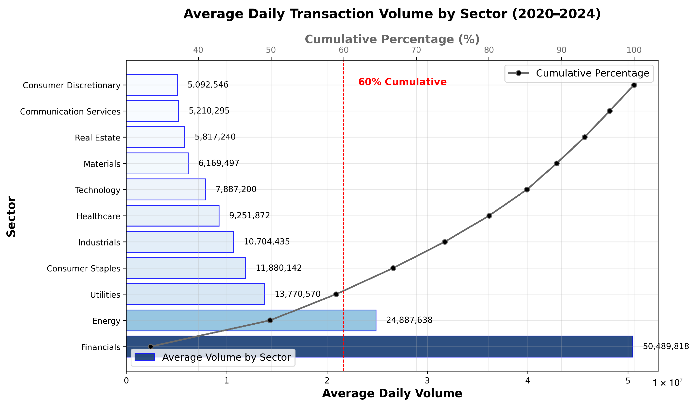
Data on sectors were collected based on their trading volume of stocks between 15 June 2020 and 31 December 2024. According to Kapalu and Kodongo (2022), the COVID-19 pandemic occurred between January 2020 and June 2020; for this reason, the data were considered from 15 June. The use of daily data allowed for a more detailed analysis of asset price dynamics and improved the statistical power of the estimates as a result of the larger sample size. However, we recognize that high-frequency data may introduce a higher level of noise and market microstructure effects that are less relevant in monthly data. Using daily data increased the number of observations, thereby improving the statistical power of the analysis and enabling a more robust estimation of factor sensitivities over time. To mitigate the effects of potential noise, we ensured the consistency of data sources, excluded days with abnormal trading interruptions, and focused on portfolios constructed from highly liquid assets, such as those accounting for 60% of the trading volume. These measures helped to reduce distortions commonly associated with microstructure effects. Relative frequency and cumulative frequency calculations were performed, and a secondary axis was added to the graph to draw a line showing the cumulative percentage, using circular markers at each corresponding point. The vertical red line indicates 60% of the accumulated volume, highlighting the sectors that contributed significantly to the volume of transactions for the stocks traded in the index (Figure 1).

For the purposes of the portfolios, the stocks belonging to the 3 sectors mentioned above are taken into account, as they account for 60% of the total volume of transactions.

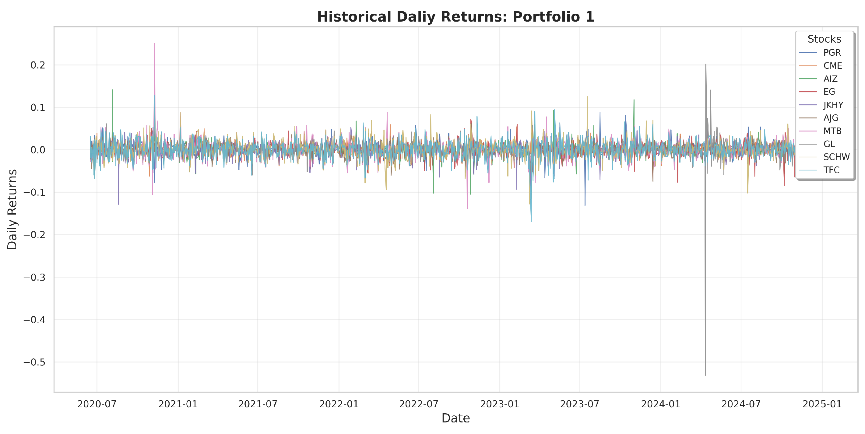
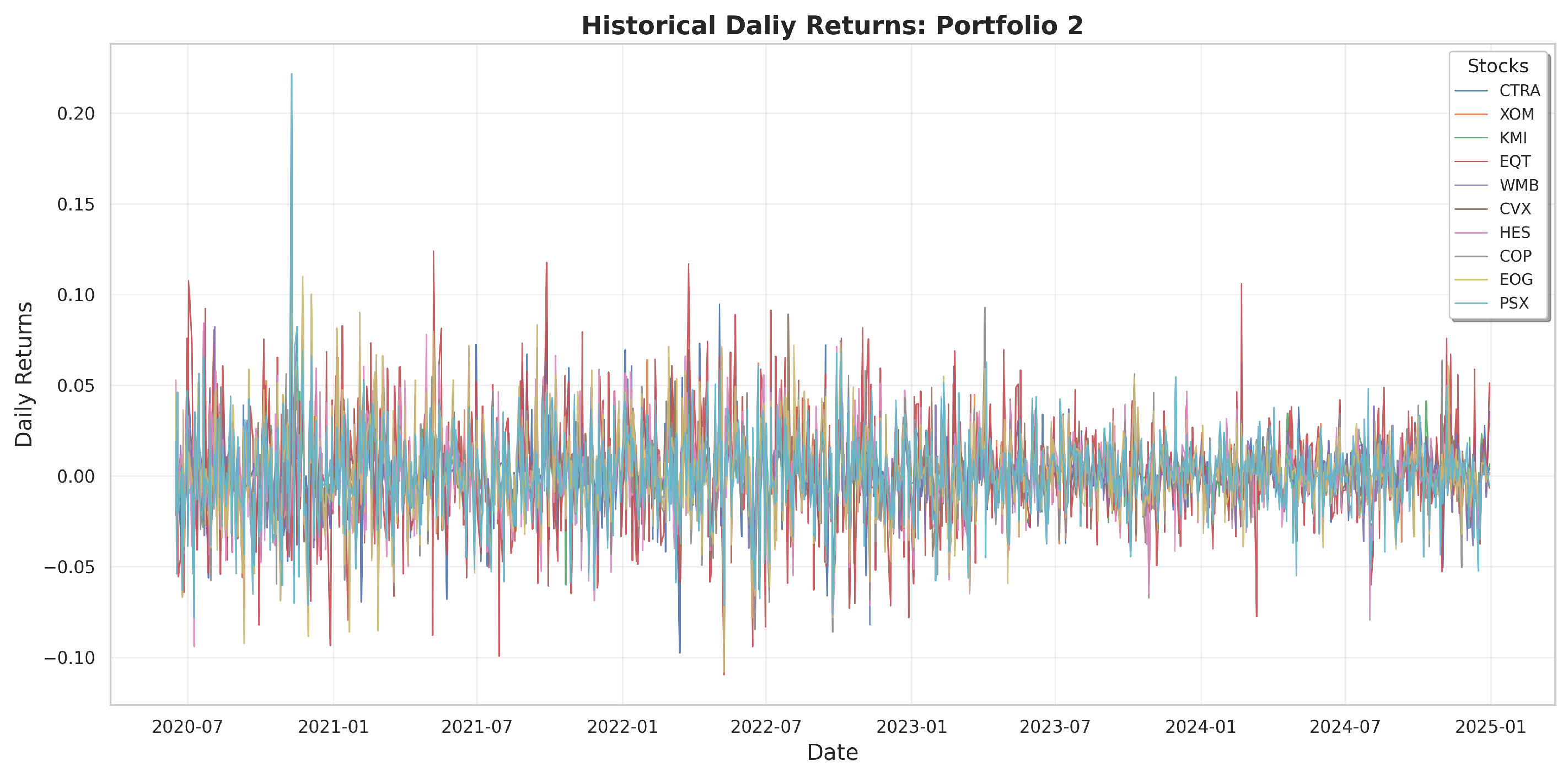
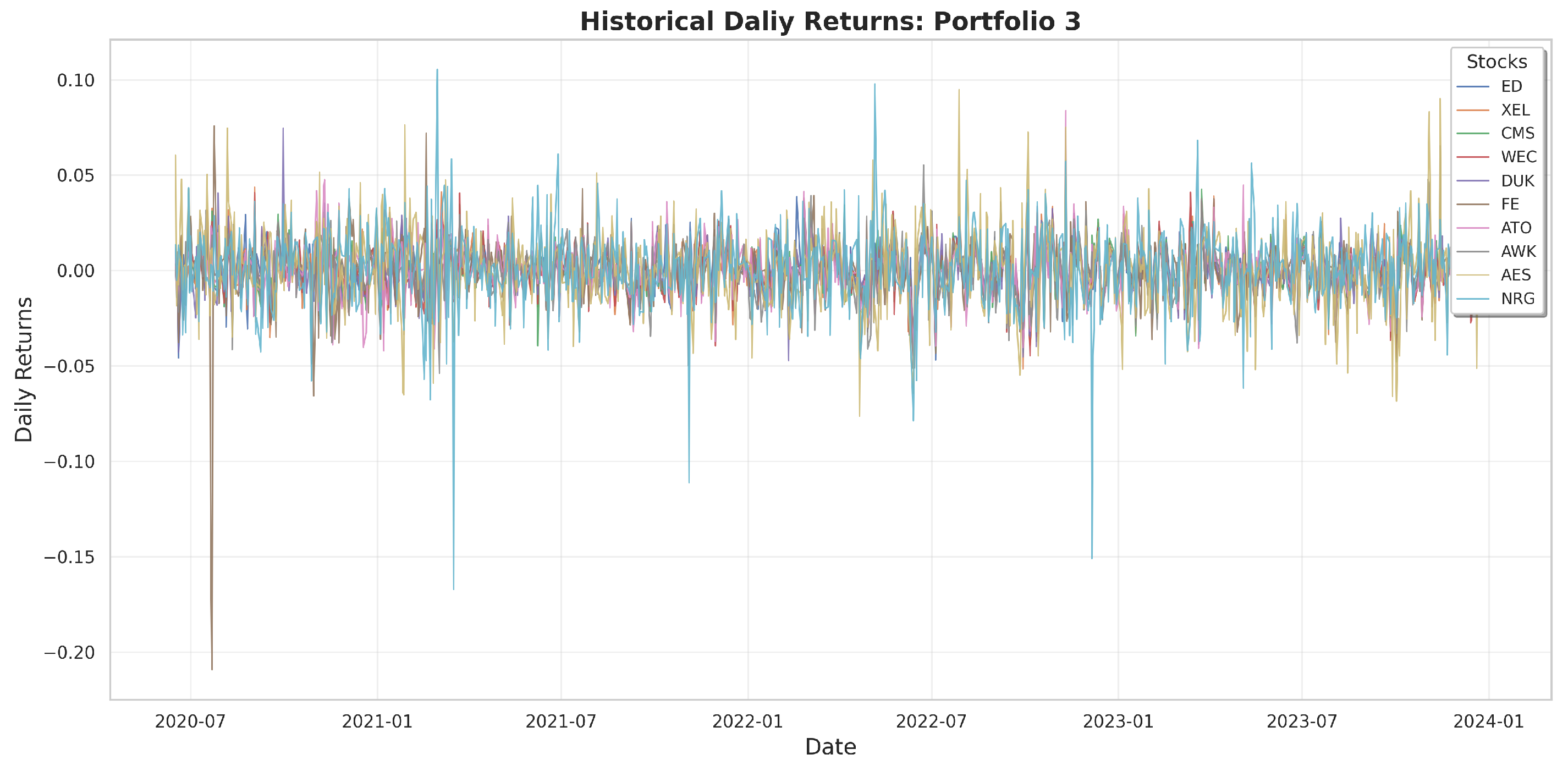
Asset selection criteria are based on sector diversification and the selection of the lowest beta ($\beta$), demonstrating the explanatory power of multifactor models when the market risk is considered as a weighting factor in the same way as the other factors. The assets selected for each portfolio are shown in

Table 2. Portfolio of financial industry: P1.

Portfolio of Financial Industry: P1
Stocks	Sub-Industry	Beta $\mathit{\beta }$
PGR	Property & Casualty Insurance	0.351
CME	Financial Exchanges & Data	0.561
AIZ	Multi-line Insurance	0.563
EG	Reinsurance	0.614
JKHY	Transaction & Payment Processing Services	0.639
AJG	Insurance Brokers	0.725
MTB	Regional Banks	0.745
GL	Life & Health Insurance	0.808
SCHW	Investment Banking & Brokerage	0.963
TFC	Diversified Banks	1.038

,

Table 3. Portfolio of energy industry: P2.

Portfolio of Energy Industry: P2
Stocks	Sub-Industry	Beta $\mathit{\beta }$
CTRA	Oil & Gas Exploration & Production	0.198
XOM	Integrated Oil & Gas	0.877
KMI	Oil & Gas Storage & Transportation	0.921
EQT	Oil & Gas Exploration & Production	1.064
WMB	Oil & Gas Storage & Transportation	1.077
CVX	Integrated Oil & Gas	1.079
HES	Integrated Oil & Gas	1.162
COP	Oil & Gas Exploration & Production	1.223
EOG	Oil & Gas Exploration & Production	1.285
PSX	Oil & Gas Refining & Marketing	1.318

and

Table 4. Portfolio of utilities industry: P3.

Portfolio of Utilities Industry: P3
Stocks	Sub-Industry	Beta $\mathit{\beta }$
ED	Multi-Utilities	0.348
XEL	Multi-Utilities	0.4
CMS	Multi-Utilities	0.405
WEC	Electric Utilities	0.437
DUK	Electric Utilities	0.456
FE	Electric Utilities	0.489
ATO	Gas Utilities	0.672
AWK	Water Utilities	0.691
AES	Independent Power Producers & Energy Traders	1.07
NRG	Independent Power Producers & Energy Traders	1.086

, forming three portfolios of 10 assets each for the financial, energy, and utilities sectors, respectively. The daily returns of these assets, organized in portfolios, are shown in Figure 2, Figure 3 and Figure 4 for the period from 2020 to 2024.

The beta coefficient $\beta$ quantifies the sensitivity of the returns of stocks ($R_a$) relative to the returns of a reference market index ($R_m$). Mathematically, beta $\beta$ is expressed in Equation (1):

$$\beta ={\displaystyle \frac{\mathrm{Cov}(R_a,R_m)}{\mathrm{Var}\left(R_m\right)}}$$

(1)

where:

• $R_a$ represents the returns of the stock.
• $R_m$ represents the returns of the reference market index.
• $\mathrm{Cov}(R_a,R_m)$ refers to the covariance between the stock’s returns and the market’s returns.
• $\mathrm{Var}\left(R_m\right)$ represents the variance of the market’s returns.

In Equation (1), beta ($\beta$) is obtained using the OLS regression parameter.

This analysis focuses on industries with the highest number of transactions in the S&P500 index of the United States of America market. Historical market data are used with the lowest beta criteria to ensure that the results obtained adequately reflect economic conditions. To apply the models, the CAPM equations, the Fama and French three-factor model, and the Fama and French five-factor model are used.

Table 5. Methods for obtaining variables and factors of the CAPM, FF3 model, and FF5 model.

Variable	Description	Method	Applying
Rf	Risk-free rate, use of sovereign bonds.	10-year sovereign bonds.	Linear regression (CAPM) and multiple regression (FF3 and FF5) as factors explaining asset performance relative to the market.
(Rm-Rf)	Excess market return, which is the market return minus the risk-free rate.	Kenneth R. French database, market return and the risk-free rate.	Linear regression (CAPM) and multiple regression (FF3 and FF5) as factors explaining asset performance relative to the market.
SMB	Size premium, the difference between the performance of small and big companies.	Kenneth R. French database.	Multiple regression for FF3 and FF5 models, representing the impact of firm size on returns.
HML	The value premium is defined as the difference between the performance of companies with high and low book-to-market ratios.	Multiple regression for FF3 and FF5 models, explaining how firm value affects expected returns.
RMW	The profitability factor is the difference between the returns of companies with high and low operating profitability, which is measured by the profit margin.	Kenneth R. French database (only for FF5).	Multiple regression of the FF5 model, measuring how profitability affects expected returns.
CMA	Investment factor, calculated as the difference between the performance of companies with conservative and aggressive investment strategies.	Kenneth R. French database (only for FF5).	Multiple regression of the FF5 model, representing the effect of investment on company returns.
Historical performance	Historical data.	Yahoo Finance databases.	Linear regression (CAPM) and multiple regression (FF3 and FF5) to predict expected returns.
Beta ($\beta$)	Sensitivity of an asset’s performance to changes in the market.	Historical data.	Consideration of the calculation of the expected return in the CAPM and in the SMB, HML, and other factors in the FF3 and FF5 models.
Root mean square error (RMSE)	Error metric that evaluates the difference between predicted and actual values.	For each of the models.	This allows us to evaluate the accuracy of the predictions of each model and to compare the performance between models.
Mean absolute error (MAE)	Error metric that measures the average absolute difference between predicted and observed values.	For each of the models.	This is used to evaluate the performance of the models in terms of prediction accuracy, completing the evaluation together with the RMSE.

below details the variables and factors present in the models analyzed.

The model equations are detailed below:

Equation (2) is used for the CAPM:

$$R_{it}-R_f={\alpha }_i+{\beta }_i(R_m-R_f)+{ϵ}_{it}$$

(2)

where:

• $R_{it}$ corresponds to the expected return, in equilibrium, of asset i at time t.
• $R_f$ is the risk-free return.
• $(R_m-R_f)$ corresponds to the excess return on the market.
• ${\beta }_i$ represents the beta, which measures the degree of sensitivity of the asset with respect to the market.
• ${\alpha }_i$ is the intercept.
• ${ϵ}_{it}$ is a random error term, which captures the deviations not explained by the model.

Equation (3) is used for FF3:

$$R_{it}-R_f={\alpha }_i+{\beta }_i·(R_m-R_f)+s_t·{\mathrm{SMB}}_t+h_t·{\mathrm{HML}}_t+{ϵ}_{it}$$

(3)

• $R_{it}$ corresponds to the expected return, in equilibrium, of asset i at time t.
• $R_f$ is the risk-free return.
• ${\beta }_i$, $s_t$, and $h_t$ represent the degree of sensitivity of the asset with respect to the associated factor.
• ${\alpha }_i$ is the intercept.
• ${ϵ}_{it}$ is a random error term, which captures deviations not explained by the model.
• $(R_m-R_f)$ corresponds to the excess return on the market.
• ${\mathrm{SMB}}_t$ is the size premium (small minus big).
• ${\mathrm{HML}}_t$ is the value premium (high minus low).

Equation (4) is used for FF5:

$$R_{it}-R_f={\alpha }_i+{\beta }_i·(R_m-R_f)+s_t·{\mathrm{SMB}}_t+h_t·{\mathrm{HML}}_t+r_t·{\mathrm{RMW}}_t+c_t·{\mathrm{CMA}}_t+{ϵ}_{it}$$

(4)

• $R_{it}$ corresponds to the expected return, in equilibrium, of asset i at time t.
• $R_f$ is the risk-free return.
• ${\beta }_i$, $s_t$, $h_t$, $r_t$, and $c_t$ represent the sensitivity of the asset to the associated factor.
• ${\alpha }_i$ is the intercept.
• ${ϵ}_{it}$ is the random error term, which captures the deviations not explained by the model.
• $(R_m-R_f)$ corresponds to the excess return on the market.
• ${\mathrm{SMB}}_t$ is the size premium (small minus big).
• ${\mathrm{HML}}_t$ is the value premium (high minus low).
• ${\mathrm{RMW}}_t$ is the operating profitability factor (robust minus weak), capturing the difference in returns between companies with high and low operating profitability.
• ${\mathrm{CMA}}_t$ is the investment factor (conservative minimum aggressive), capturing the difference in returns between companies that invest conservatively and aggressively.

In asset pricing models, the beta (${\beta }_{mkt}$, ${\beta }_{smb}$, ${\beta }_{hml}$, ${\beta }_{rmw}$, and ${\beta }_{cma}$) represents the degree of sensitivity of an asset’s return to each of the factors in the model (MKT, SMB, HML, RMW, and CMA). In the case of the CAPM, the beta measures how an asset’s performance responds to movements in the overall market (market premium $R_m-R_f$).

For the FF3 model, beta ${\beta }_{smb}$ measures the sensitivity of asset performance to differences in returns between portfolios constructed according to market capitalization (small versus large companies), and beta ${\beta }_{hml}$ measures the sensitivity of asset performance to differences between portfolios constructed according to the book-to-market ratio (book value versus market value).

Finally, for the FF5 model, beta ${\beta }_{rmw}$ measures how much the asset return changes when the RMW factor return (robust versus weak return) changes by one unit, and beta ${\beta }_{cma}$ measures how much the asset return changes when the CMA factor return (conservative versus aggressive investment) changes by one unit. Specifically, beta $\beta$ represents the volatility of the asset relative to the factor to which it is linked. In the algorithm, the beta ($\beta$) factor is calculated by fitting a multiple linear regression (OLS), in which the excess return of the stock is modeled as a function of the market (MKT), size (SMB), value (HML), yield (RMW), and investment (CMA) factors defined by Fama and French. The estimated coefficients in this regression represent the sensitivity of the stock to each of these factors and are obtained directly from the fitted model using the statsmodels library. The sm.ols() function of statsmodels (used in the algorithm) uses ordinary least squares (OLS) to estimate the coefficient beta $\beta$, as shown in Equation (5):

$$\widehat{\beta }={\left(X^{T}X\right)}^{-1}{X}^{T}y$$

(5)

where:

• X represents the matrix of the factor values (MKT, SMB, HML, RMW, and CMA).
• y denotes the vector of excess returns of the asset.
• $\beta$ refers to the estimated betas.

Regarding the government bond corresponding to the risk-free return considered, a value of 4.418% is selected for a 10-year US bond. Values are considered for time horizons of 3, 5, and 10 years, which, when compared, show a minimum variation in returns. Due to the stability that this variable represents, the one with the highest value is selected, being 4.257% for 3 years and 4.286% for 4 years, and 4.418% is the one selected with a 10-year extension.

The method is based on a correlational approach to the variables, applying the factors of each model. The results are evaluated by making a direct comparison of the following error metrics: the root mean square error (RMSE) and mean absolute error (MAE) (Zografopoulos et al., 2025).

(a) RMSE: The root mean square error (RMSE) quantifies the difference between the expected and observed performance, giving greater weight to larger errors by squaring the differences. A lower RMSE indicates that the predicted data are closer to the actual data. A higher RMSE indicates a greater difference between the predicted and actual data (Lin & Huang, 2020).

$$\mathrm{RMSE}=\sqrt{{\displaystyle \frac{1}{n}}\sum _{i=1}^n{\left(y_{\mathrm{exped},i}-y_{\mathrm{real},i}\right)}^2}$$

(6)

In Equation (6), $y_{\mathrm{real}}$ represents the actual values of the test set ($y_{\mathrm{test}}$), and $y_{\mathrm{exped}}$ is the output of the model predict($X_{\mathrm{test}}$).flatten(), which is the prediction made by the model.

(b) MAE: The mean absolute error is one of the most popular measures of forecast accuracy. The MAE is the average of the absolute errors between the predicted and observed values, as shown in Equation (7):

$$\mathrm{MAE}={\displaystyle \frac{1}{n}}\sum _{i=1}^n\left|y_{\mathrm{real},i}-y_{\mathrm{expect},i}\right|$$

(7)

The RMSE and MAE (Chahuán-Jiménez, 2024) are suitable metrics for fitting the model. This approach allows us to identify the model that generates the lowest error and best fits the actual data in the portfolios.

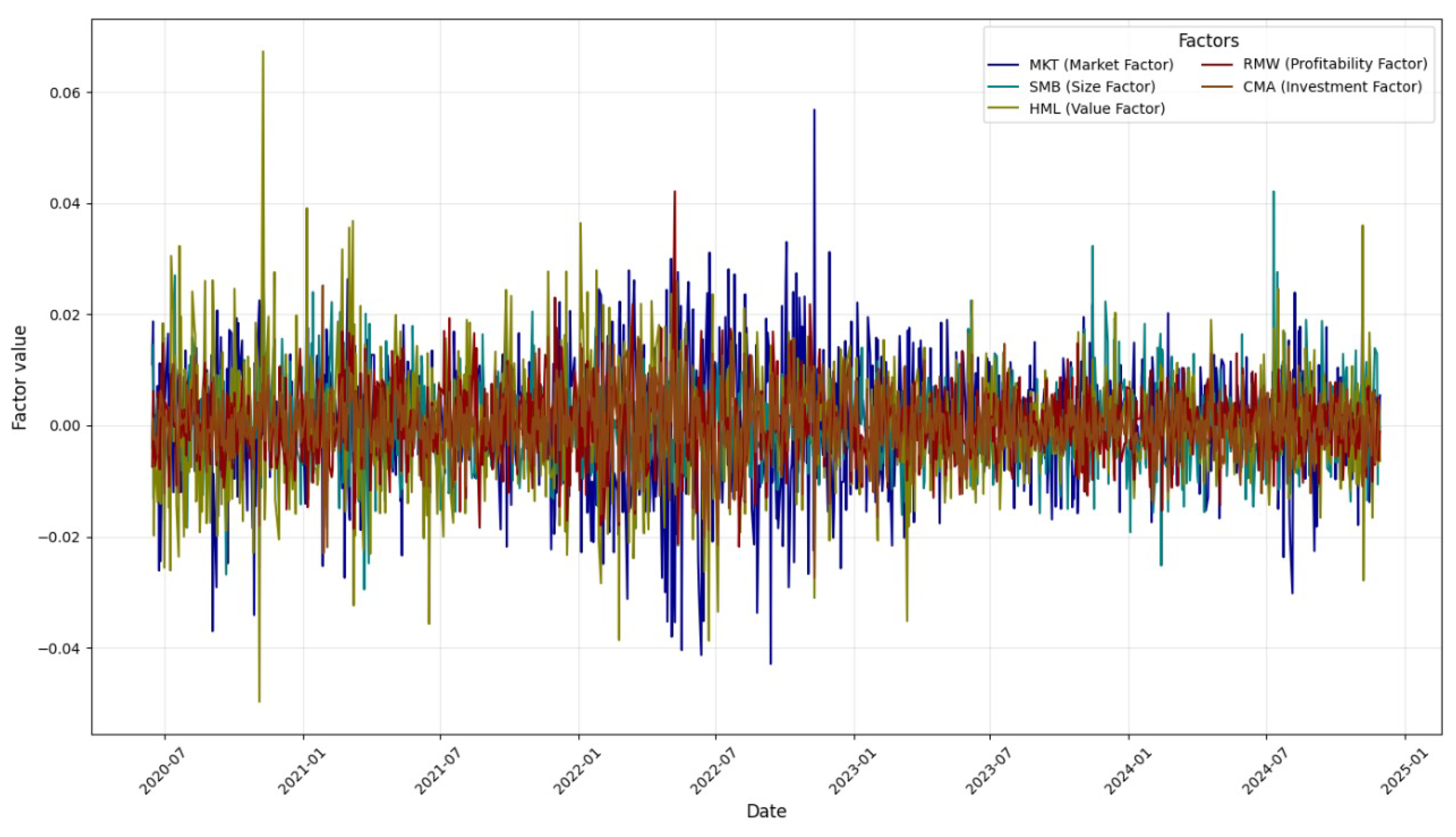
3. Results

The results first show the differences in the factors calculated for the methods used to value the assets, as shown in Figure 5.

All of the market factors calculated for the CAPM have a positive sign and are statistically significant, as shown in

Table 6. CAPM regression result.

Portfolio	Intercept	Factor MKT	Adjusted ${\mathit{R}}^2$
P1	−0.02	0.41 **	0.07
P2	0.01	0.42 **	0.06
P3	−0.02	0.26 *	0.03

Note: * $p<0.1$; ** $p<0.05$.

.

As shown in Table 6, for portfolio P1, the market coefficient is 0.41, and it is statistically significant at 1% (**), indicating a moderate sensitivity to market movements. The intercept is −0.02, although it is not significant, and the adjusted $R^2$ is 0.07, meaning that the model explains 7% of the variability in returns. For portfolio P2, the MKT coefficient is slightly higher (0.42 **) and significant at 1%, with a non-significant intercept of 0.01. The adjusted $R^2$ is 0.06, showing an explanatory power similar to that of P1. For portfolio P3, the MKT coefficient is lower (0.26 *) and significant at 10%, with a non-significant intercept of −0.02. The adjusted $R^2$ is 0.03, indicating that the model has a lower ability to explain returns for this portfolio than for the other portfolios. In summary, the results show that the market factor has a significant impact on portfolio returns, although the explanatory power of the models is limited, as indicated by the low adjusted $R^2$ values.

Table 7. FF3 regression result.

Portfolio	Intercept	MKT	SMB	HML	Adjusted ${\mathit{R}}^2$
P1	−0.02	0.58 ***	−0.02	0.7 ***	0.2
P2	−0.02	0.66 ***	−0.14	0.78 ***	0.19
P3	−0.02	0.29 **	0.16	0.42 **	0.13

Note: ** $p<0.05$; *** $p<0.01$.

presents the estimated coefficients of the regressions based on the Fama and French (FF3) three-factor model applied to the three portfolios (P1, P2, and P3), which show the following: Portfolio P1: The market coefficient (MKT) is positive (0.58) and highly significant at 1%, indicating a strong sensitivity to the market factor. The value factor (HML) also has a positive coefficient (0.7) with high significance, indicating that this portfolio is exposed to stocks with high book-to-market ratios. The SMB coefficient is negative but insignificant, indicating that the size of the company does not have a clear effect. The model explains about 20% of the return variability (the adjusted $R^2$ is 0.20). Portfolio P2: This behaves similarly to P1. The market factor has a higher coefficient (0.66 ***) and is also statistically significant at 1%. The coefficient of the HML factor is even higher (0.78 ***), indicating a strong tilt toward value stocks. Although the coefficient of the SMB factor is negative (−0.14), it does not reach statistical significance. The adjusted $R^2$ is 0.19. Portfolio P3: In this portfolio, the coefficients are still positive for MKT (0.29 **) and HML (0.42 **), which are both significant at 5%, showing a lower sensitivity than those for portfolios P1 and P2 but still being relevant. The SMB factor has a positive coefficient (0.16), although it is not statistically significant. The model explains 13% the variability of the returns (the adjusted $R^2$ is 0.13).

Table 8. FF5 regression result.

Portfolio	Intercept	MKT	SMB	HML	RMW	CMA	Adjusted ${\mathit{R}}^2$
P1	−0.02	0.57 ***	−0.13	0.758 ***	−0.27	0.14 **	0.20 **
P2	−0.02	0.67 ***	0.00	0.71 ***	0.3324 **	0.1711 **	0.19 **
P3	−0.02	0.29 **	0.13 **	0.36 **	−0.11	0.30 **	0.15 **

Note: ** $p<0.05$; *** $p<0.01$.

shows the estimated coefficients of Fama and French’s five-factor model applied to the three portfolios (P1, P2, and P3), indicating the following: Portfolio P1: The coefficient of the market factor (MKT) is positive (0.57) and highly significant at 1%, indicating a strong sensitivity to market returns. The value factor (HML) is also positive and significant (0.758), reflecting a clear bias toward value stocks. However, the SMB (−0.13) and RMW (−0.27) factors are not statistically significant, while the investment factor (CMA) has a positive coefficient (0.14 **) and is significant at 5%, indicating a certain preference for companies with conservative investment policies. The adjusted $R^2$ is 0.20 **, which means that the model explains 20% of the variability of the returns of this portfolio. Portfolio P2: The market coefficient is even higher (0.67 ***) and highly significant. As in P1, the value factor (HML) has a high coefficient (0.71 ***) and is highly significant. The coefficient of the profitability factor (RMW) is positive and significant (0.3324 **), suggesting exposure to companies with high operating profitability. The investment factor (CMA) is also significant (0.1711 **), while SMB has no effect (coefficient of 0.00). The model has an adjusted $R^2$ of 0.19 **, indicating an explanatory power similar to that of P1. Portfolio P3: This portfolio has a lower market coefficient (0.29 **), although it is still significant. The value factor (HML) retains its significance (0.36 **), although to a lesser extent than in P1 and P2. Unlike the other portfolios, the size factor (SMB) has a positive and significant coefficient (0.13 **), indicating a bias toward companies with lower capitalization. The capitalization factor (CMA) is also relevant (0.30 **), while the RMW is insignificant (−0.11). The adjusted $R^2$ is 0.15 **, indicating a moderate explanatory power.

The results confirm the relevance of the value factor (HML) as a common and significant determinant in all portfolios, while the factors of profitability (RMW) and investment (CMA) provide additional explanations in P2 and P3. The size factor (SMB) seems to be relevant only in portfolio P3. The FF5 model improves the fit compared to versions with fewer factors, as can be seen in the adjusted $R^2$ values, which range between 15% and 20%.

The progressive inclusion of factors from the one-factor model to the FF5 model allows for a better explanation of portfolio returns. However, the increase in the adjusted $R^2$ between FF3 and FF5 is marginal, suggesting that, while the additional factors have some relevance, the three-factor model already captures a significant portion of the variability. Since the SMB factor is not significant compared to the others, we developed an intermediate model between FF3 and FF5 with four factors. The results associated with this model are presented in

Table 9. FF4 regression result.

Portfolio	Intercept	MKT	HML	RMW	CMA	Adjusted ${\mathit{R}}^2$
P1	−0.02	0.54	0.68	−0.16	0.14	0.19
P2	−0.02	0.67	0.71	0.33	0.17	0.20
P3	−0.02	0.31	0.44	−0.23	0.30	0.14

.

No variations affecting the model’s effectiveness are observed, regardless of whether the factor associated with company size is considered or disregarded.

The comparison between the mean absolute error, applied to each of the models under study for the proposed portfolios, is shown in

Table 10. MAE.

Sector	CAPM	FF3	FF5	FF4
Financial	2.55%	1.95%	2.01%	2.14%
Energy	2.53%	1.53%	1.50%	1.50%
Utilities	3.38%	3.17%	3.15%	3.02%

.

Table 10 shows that the model with the highest error in terms of the MAE is the CAPM, with an MAE ranging from 2.55% to 3.38%. In comparison, the models with the lowest mean absolute errors are the FF5 and FF4 models, with values ranging from 1.50% to 3.15% and from 1.50% to 3.02%. The fact that the Capital Asset Pricing Model performs worst in this accuracy comparison is in line with a study by Alaoui Taib and Benfeddoul (2023), who were able to conclude from the regression results of their study that the single-factor model presents the worst performance of the three; additionally, when comparing FF3 with FF5 and the FF4 model in this research, the results obtained confirmed the general superiority of the FF5 and FF4 models.

Table 11. RMSE metric.

Sector	CAPM	FF3	FF5	FF4
Financial	2.82%	2.17%	2.34%	2.47%
Energy	2.59%	1.62%	1.59%	1.59%
Utilities	3.72%	3.42%	3.41%	3.33%

compares the performance of the models applied to the financial, utilities, and energy sectors using the RMSE metric.

RMSE (root mean square error) values were obtained for the three financial models applied to different industries. Looking at the overall results, it can be observed that the CAPM is the least accurate, with an RMSE ranging from 2.82% to 3.72%, reflecting limited empirical performance. In contrast, the FF5 model has lower RMSE indices, with values ranging from 1.59% to 3.41%, closely followed by the FF4 model, with values ranging from 1.50% to 3.33%, and the FF3 model, with values ranging from 1.62% to 3.42%. This indicates that both Fama and French models significantly improve the predictive accuracy compared to the CAPM. When analyzing the results by industry sector, the FF3 model is found to be the most accurate for the financial sector, with an RMSE of 2.17%, slightly ahead of FF5, which has an RMSE of 2.34%, suggesting that the three-factor model is better at describing returns in this sector. For the utilities industry, the FF4 model shows the best fit, with an RMSE of 3.33%, although the difference from the FF3 model, whose RMSE is 3.42%, excluding the size of the companies, reduces the error margin in this sector.

The analysis confirms that the FF4 and FF5 models (and the FF3 model) have a greater explanatory power than the CAPM in the sectors analyzed. However, the effectiveness of each model depends on the specific characteristics of each industry. Therefore, although demonstrating that the risk factors captured by the multifactor models generate differences in their predictive capacity, it depends on the sector in which the investment is made; in general, the models that include more factors generate less error.

4. Discussion

Referencing studies applied in other markets provides an enriching context. For example, while a study in the Australian market found that the FF5 model explained a greater number of anomalies, and research in the Chinese market also suggested a superiority of the FF5 model, our results indicate a slight advantage of the FF3 model in the US financial sector. These differences highlight the dependence of model performance on the specific characteristics of each market. The applicability of the CAPM, for instance, is considered adequate in developed markets, but it faces limitations in emerging markets due to factors such as country risk. Therefore, the variation in the behavior of the models between markets underscores the need to adapt and evaluate asset pricing models in the specific context in which they are applied. The absence of a universal consensus on the optimal model reinforces the importance of empirical research such as that presented here, which seeks to determine the model with the best fit for specific sectors within a given market.

Handri (2023), in his analysis of the CAPM in different industries, reported a mean squared error (MSE) ranging from a maximum of 12.5% to a minimum of 2.47%. The mean absolute error (MAE) ranged from 9.07% to 1.92%. Similarly, Khoa and Huynh (2023b) analyzed the performance of the Fama and French three-factor model and found that the RMSE ranged from 2.81% to 3.15%. In comparison, the CAPM exhibited a slightly higher RMSE, ranging from 2.48% to 3.76%.

A study conducted by Kostin et al. (2022) analyzed the validity of both the Fama and French models in crisis contexts, using data from energy sector firms in developed and emerging markets during the COVID-19 pandemic. The results showed that the models with more factors, that is, the FF3, FF4 (included through this research), and FF5 models in developed markets, showed differences in accuracy that were not significant. Therefore, when considering the model to be used, much depends on the sector in which the investor makes the decision to invest, since the factors will affect the fit of the model, and these factors are more sensitive in some sectors than others.

J.-L. Chen et al. (2022) found that the five-factor model of Fama and French performs better than the three-factor model (FF3) in explaining Chinese stock market returns. However, it does not fully capture the dynamics of this market. In particular, the five-factor model outperforms the three-factor model (Skočir & Lončarski, 2024), supporting the notion that the additional pricing factors incorporated into the model increase its explanatory power.

Cox and Britten (2019) concluded that, although the Fama and French five-factor model improves the explanatory power of traditional models in capturing returns on the Johannesburg Stock Exchange, three-factor models focusing on size–value or size–return are more effective in certain configurations. Furthermore, the relevance of the value–return premium was confirmed in the South African context, while the investment effect showed ambiguous results. These findings highlight the need to adapt asset pricing models to the specific characteristics of local markets. On the other hand, according to Barillas and Shanken (2017), test assets can influence the choice of the model with other metrics, and the challenge for those who advocate the use of such measures, especially those who do not attach importance to the pricing of excluded factors, remains to articulate the economic rationale for these alternative approaches.

5. Conclusions

This study focused on an empirical approach, applying the CAPM, FF3 model, and FF5 model to key companies in sectors that contribute significantly to the transaction volume of the Standard & Poor’s 500 Index (S&P 500) of the US financial market. The selection of sectors and companies was based on transaction volume, with the financial, utilities, and energy sectors selected, and the companies selected were those that were less sensitive to market changes, i.e., those with a lower beta.

The objective of this study was to compare the CAPM, FF3 model, and FF5 model in different sectors of the US market in order to value assets by accuracy, considering the lowest error. The results obtained consistently showed that the multifactor models (FF3, FF5, and FF4 developed for this study) had a higher predictive accuracy than the CAPM, which is consistent with the literature that points out the empirical limitations of the single-factor model. When using one of the FF models, it is necessary to identify the sector in which the assets are valued, since sectors are sensitive to the factors included in the models. In terms of the mean absolute error (MAE), the CAPM had the highest error, ranging from 2.55% to 3.38%, while the error of the FF5 model ranged from 1.50% to 3.15%, and that of the FF4 model ranged from 1.50% to 3.02% for the energy and utilities sectors. Similarly, for the root mean square error (RMSE), the CAPM had values between 2.82% and 3.72%, while the FF5 model had values between 1.59% and 3.41%, and the FF4 model had values between 1.59% and 3.33%, closely followed by the FF3 model, with values between 1.62% and 3.42%; the same results were obtained for the financial sector, where the lowest error was found for the FF3 model.

The financial sector was more sensitive to market conditions and asset valuations than the other sectors. However, the better performance of FF5 and FF4 in the energy and utilities sectors could indicate that profitability and investment strategies play a more important role in determining returns in these sectors, possibly influenced by long-term economic cycles and capital-intensive investments.

The limited explanatory power of the CAPM in all sectors can be attributed to its simplified assumptions, in particular, the assumption of perfectly efficient markets and the consideration of the market beta as the only measure of systematic risk. In contrast, the Fama and French models (FF3, FF5, and FF4) incorporate additional factors that capture specific characteristics of firms and the market, reflecting a broader and more realistic approach to asset valuation, consistent with empirical evidence that multiple dimensions of risk affect expected returns.

Although our overall results are consistent with those of other studies that favor multifactor models over the CAPM, the specific discussion by sector is limited by the lack of direct comparative literature analyzing the performance of these three models in the same S&P 500 sectors over the same period. A study conducted by Handri (2023) reported error ranges for the CAPM in different industries in Indonesia, and another study analyzed the FF3 model, but these did not focus on the specific sectors or US market examined in our study. However, it is interesting to note that a study of the energy sector during the COVID-19 pandemic found that the FF5 model slightly outperformed FF3 in developed markets, for example, in the case of leading companies such as ExxonMobil, Chevron, and Shell, suggesting a better ability to explain the variation in returns. Despite this limitation, our results clearly indicate that the effectiveness of each model is inextricably linked to the specifics of each industry.

This empirical study provides new evidence on the comparative performance of four financial asset valuation models: the Capital Asset Pricing Model (CAPM), the three-factor model (FF3), the five-factor model (FF5) developed by Fama and French, and the four-factor model (FF4) presented in this study. These models enable us to estimate the expected return on investments based on different sources of systematic risk. Furthermore, their ability to explain observed market returns can be interpreted as empirical evidence for or against market efficiency and asset price accuracy. Our results show that multifactor models with three, four, or five factors outperform other models. The size premium, which is the difference in performance between small and large companies, was not significant in the calculations performed in this research. Therefore, our future research will focus on adjusting the model to achieve the highest possible accuracy for this specific factor.

It is important to recognize the inherent limitations of this study. We focused on companies with low market sensitivity (low beta) within specific S&P 500 sectors. Therefore, caution should be exercised when generalizing these results to other sectors or companies with different risk profiles. Future research could explore the validity of these models in a wider range of industries and market sensitivities.