Article

The Dynamic Return and Volatility Spillovers among Size-Based Stock Portfolios in the Saudi Market and Their Portfolio Management Implications during Different Crises

by
Nassar S. Al-Nassar
Department of Economics and Finance, College of Business and Economics, Qassim University, Buraydah 51452, Saudi Arabia
Int. J. Financial Stud. 2023, 11(3), 113; https://doi.org/10.3390/ijfs11030113
Submission received: 25 July 2023 / Revised: 25 August 2023 / Accepted: 31 August 2023 / Published: 12 September 2023

Abstract

:
This study contributes to the ongoing debate on the size effect and size-based investment styles by investigating the return and volatility spillovers and time-varying conditional correlations among Saudi large-, mid-, and small-cap indices. To this end, we utilize the weekly returns on the MSCI Saudi large-, mid-, and small-cap indices over a long sample period, spanning several crises. The econometric approach that we use is a VAR-asymmetric BEKK-GARCH model which accounts for structural breaks. On the basis of the VAR-asymmetric BEKK-GARCH model estimation results, we calculate portfolio weights and hedge ratios, and discuss their risk management implications. The empirical results confirm the presence of unilateral return spillovers running from mid- to small-cap stocks, while multilateral volatility spillovers are documented, albeit substantially weakened when accounting for structural breaks. The time-varying conditional correlations display clear spikes around crises, which translate to higher hedge ratios, increasing the cost of hedging during turbulent times. The optimal portfolio weights suggest that investors generally overweight large caps in their portfolios during uncertain times to minimize risk without lowering expected returns. The main takeaway from our results is that passively confining fund managers to a particular size category regardless of the prevailing market conditions may lead to suboptimal performance.

1. Introduction

The size effect documented by Banz (1981), who shows that small-capitalization stocks outperform their larger-capitalization counterparts on a risk-adjusted basis over a long period of time, has attracted the attention of finance academics and professionals alike. In their seminal work, Fama and French (1993, 2015) introduced the size factor as an integral component of their well-known three- and five-factor asset pricing models. This discovery motivated the finance industry to develop factor investing styles and construct factor-based stock market indices, particularly size-based indices that are used as benchmarks by an entire category of small-cap mutual funds (Keim 1999; Reinganum 1983). While several studies scrutinized and challenged the size effect, and some showed that it vanished in the early 1980s (Hirshleifer 2001; for example, Chan et al. 2000; Eleswarapu and Reinganum 1993), Reinganum (1999) noted that “far from being dead, market capitalization matters very much”. van Dijk (2011) documented that the size premium in the US has been meaningfully present in recent years and called for more empirical work addressing the size effect not only in the US but also in other stock markets that operate in advanced and emerging economies. De Moor and Sercu (2013) documented a persistent size effect using a sample of stock markets in 39 countries across several geographic regions. Recently, Asness et al. (2018) demonstrated that the size effect is strongly evident when taking the quality of firms into consideration.
The prominence of the size effect is clearly manifested in the cross-equity price dynamics among different-sized portfolios. Lo and MacKinlay (1990a, 1990b) documented an asymmetric positive cross-serial correlation running from the return of large stock portfolios to their small-sized counterparts. Conrad et al. (1991) argued that, because stock price volatility is driven by the rate at which information flows to the market, as suggested by Ross (1989), a close investigation of the differential predictability of the conditional variances of large compared to small firms’ returns is warranted to understand how information is incorporated across different-sized firms. Conrad et al. (1991) confirmed the asymmetric (unidirectional) spillovers of returns from large to small stocks and found that the same asymmetry also applies to volatility spillovers. Subsequent studies, however, arrived at mixed results regarding the spillover direction. Chelley-Steeley and Steeley (1996) and Harris and Pisedtasalasai (2006) confirmed the asymmetric transmission of return and volatility from large to small stocks in the UK, while Harris and Pisedtasalasai (2006) found limited feedback from the portfolios of smaller stocks to the portfolios of larger stocks but only in subsamples. Similarly, Koulakiotis et al. (2016) found mild asymmetry in the cross-correlations of returns and residuals, while volatility spillovers exhibited a feedback effect among large, medium, and small stocks, especially during the postcrisis period in the Greek stock market. While Reyes (2001) and Ewing and Malik (2005) showed that there is no causality between large and small stock returns in either direction, they found asymmetric volatility spillovers running from the large to the small stock portfolio in the Japanese and US stock markets, respectively. Ewing and Malik (2005), however, showed that these spillover effects are eliminated when structural breaks are taken into consideration. Constructing two portfolios on the basis of the size of firms in the Spanish market, Marcelo et al. (2008) found a bilateral volatility spillover that also vanishes when breaks are accounted for. Karmakar (2010) and Jena et al. (2021) documented bilateral spillovers among large, medium, and small firms’ returns and volatility in the Indian market.
Against this background, awareness of the return and volatility linkages among size-based portfolios and a clear understanding of their nature and sources is of immense importance. This is because these linkages carry significant implications for asset allocation and risk management decisions. In this context, Reinganum (1999) argued that fund managers can improve their performance by dynamically revising allocations to different capitalization stocks and cautions against restricting fund managers to a narrow capitalization range. Notwithstanding the well-documented size effect, Wang et al. (2014) maintained that the performance of different capitalization categories varies over time, leading each size category to alternate in and out of favor. From the perspective of international portfolio diversification, Huang (2007) showed that small caps exhibit lower correlation with both large and small caps across different developed countries, which implies that potential diversification gains may be achieved through international investment in small-cap stocks.
While several studies have examined the return and volatility linkages among the stocks of large, medium, and small firms listed within the same stock market, only a few focused on emerging markets (Marshall and Walker (2002) for the Chilean Stock market and Karmakar (2010) and Jena et al. (2021) for the Indian stock market). Moreover, most papers did not quantify the ramifications of the dynamics of these linkages on portfolio management. Indeed, Ewing and Malik (2005) conducted the only study that explicitly investigated portfolio allocation implications across stocks with different capitalizations; however, they neglected how portfolio allocation changes over time. Given the scarcity of studies in this realm, particularly those based on emerging stock markets, we believe that the Saudi stock market constitutes an appropriate setting to expand our understanding of the dynamic linkages among different-sized portfolios and their associated portfolio and risk management implications for the below-described reasons.
First, the Saudi stock exchange has achieved remarkable progress in recent years, becoming the eighth largest stock market in the world and the third largest among its emerging market counterparts after relaxing the restrictions imposed on foreign investors to access the Saudi market. Second, the inception of a parallel market (NOMU) with less stringent listing requirements now offers small and medium-sized enterprises (SMEs) access to equity finance and reduces their debt reliance. By assuming that role, NOMU serves as a feeder to the main market. In fact, most companies that were initially listed in the parallel market have successfully transitioned their shares to the main market (Al-Nassar and Makram 2022). The continuation of NOMU in performing that role will increase the number of companies that fall within the small-cap category in the main market, thereby boosting their representation in stock market indices, which will ultimately be tracked by mutual and exchange traded funds. Third, Katiyar and Dabake (2019) reported that Saudi small-cap stocks underperformed compared to their large- and mid-cap counterparts from November 2016 to April 2019, leading to a drag on the performance of several factor strategies. Moreover, they suggested that underweighting the allocation to small-cap stocks would have improved the performance of factor-based strategies, which is inconsistent with the conventional wisdom that small-cap stocks outperform their large-cap counterparts on average. Fourth, there has been an increase in studies on the spillover’s effects of oil prices on the Saudi stock market, and on the linkages between the Saudi market and other global and emerging markets. However, as far as we know, no study has addressed how the documented oil, global, and regional shocks assimilate intra-market among different-sized portfolios and whether different-sized portfolio possess hedging and diversification abilities in time of market stress.
Therefore, the aim of this study is to contribute to the literature by providing fresh evidence on the returns and volatility spillovers among large-, mid-, and small-cap indices in Saudi Arabia and their portfolio and risk management implications over a long sample period. While Al-Nassar and Makram (2022) examined the spillovers between the Saudi main and parallel markets, the spillovers among different-sized portfolios within the main market has not previously been addressed. By doing so, we extend prior studies in several ways. First, we use an extended sample period that covers the latest developments in the Saudi stock market, spanning major financial/economic crises, including the bursting of the Saudi stock market bubble in 2006, the global financial crisis (GFC), the 2014–2016 crude oil price plunge, the COVID-19 pandemic, and the Russo-Ukrainian war, allowing careful consideration of their impact on spillovers. Second, rather than constructing portfolios, we utilize large-, mid-, and small-cap MSCI indices that are widely tracked by many investment funds. Third, we employ the widely used Baba–Engle–Kraft–Kroner (BEKK) multivariate GARCH parametrization proposed by Engle and Kroner (1995). The versatility of this modeling approach enables us to account for the stochastic properties of the data, test several hypotheses regarding return and volatility spillovers, and provide estimates of conditional variances and covariances that are used as inputs to derive the dynamic optimal portfolio weights and risk minimum variance hedge ratios and track their behavior over time.
The remaining sections are as follows: Section 2 provides a background on the Saudi stock market and reviews prior related studies; Section 3 describes the dataset and sets out the econometric methodology; Section 4 presents the empirical results; Section 5 analyzes the portfolio design and risk management implications; Section 6 contains a robustness check based on Dieobold and Yilmaz approach for spillover measurement; Section 7 concludes the paper with a brief discussion of key findings.

2. Institutional Background and Review of Related Literature

2.1. Institutional Background

The Saudi government launched an official stock exchange in 1984 with the partial intention to avoid catastrophic stock market crises such as the Al-Manakh market crash that occurred in neighboring Kuwait (Butler and Malaikah 1992). Prior to the introduction of the official exchange mechanism, the trading in Saudi public companies was facilitated by unregulated brokerage offices. However, under the official exchange mechanism, rights to provide brokerage services was granted exclusively to the 12 commercial banks operating in Saudi back then (Butler and Malaikah 1992). These 12 banks constituted the Saudi share registration company (SSRC) that centrally coordinates trading orders and functions as a central clearing system. The SSRC was required to timestamp executed trades and report them daily to the share control administration department of the Saudi Arabian Monetary Agency (SAMA), the stock market regulatory body at that time. Indeed, the Saudi stock market witnessed several landmark events and developments before becoming one of the largest stock markets in the world and the largest in the MENA region.
One of the most remarkable events, in this context, is the Saudi stock market boom in the early 2000s that ended with the infamous crash of 2006 (see, Lerner et al. 2017). This dramatic stock price rally was fueled by several circumstances: the Petro-dollar inflows from the rising oil prices, the retirement of government debt, and the capital inflows arising from the withdrawal of Saudi investments from the US amid fears of possible sanctions after the 9/11 terrorist attacks (Al-Rodhan 2005). The Saudi commercial banks amplified the impact of the increased liquidity by providing margin loans that constituted a staggering 95% of the trading volume in Saudi stock market back then (Rahman et al. 2015). In addition, Rahman et al. (2015) suggested that the immediate settlement rule (T+0), which was in place at that time, is conducive for noise trading. Moreover, the lack of transparency and governance precluded the prevention of the manipulation of the price of small companies which further compounded the existing problems (AlKhaldi 2015, as cited in Lerner et al. 2017). During this critical time, the regulatory oversight of the market was passed from SAMA to the newly established Capital Market Authority (CMA) in 2004. While CMA took serious actions against traders who manipulated stock prices and implemented rules to foster transparency, it could not prevent the inevitable market crash (Lerner et al. 2017). Since then, the CMA has continuously implemented reforms that have contributed significantly to the success of the Saudi market to attract foreign investors and more listings.
The 2006 stock market crash and other critical global crises coincided with different stages of the development of the Saudi exchange. These events offer a rare opportunity to examine the spillover transmission mechanism among companies with different market capitalization to assess their susceptibility to such events and derive practical portfolio and risk management implication.

2.2. Review of Related Literature

The study of interconnectedness among financial markets is one of the mainstays of the empirical finance literature. The accumulated body of knowledge on this topic is huge and rapidly expanding. We, therefore, pragmatically limit our coverage to the studies that address the interdependencies among the MENA region and GCC member countries and other financial markets; for studies that investigated spillovers among developed and emerging markets (other than those in the MENA and GCC region), the reader may refer to Boubaker and Jouini (2014), Boubaker et al. (2016), and El Khoury et al. (2023), among others. In addition, we review the studies that focused on the size effect in other advanced and emerging markets.

2.2.1. Interdependencies among the MENA and GCC Regions and Other Financial Markets

The bulk of studies in this stream of literature fall into two sub-streams according to their main research objective. Studies in the first sub-stream focus on the relationship between the stock markets in this region and oil prices or/and oil price uncertainty (Abakah et al. 2023; Arouri et al. 2011; Abuzayed and Al-Fayoumi 2021; Awartani and Maghyereh 2013; Bani-Khalaf and Taspinar 2022; Basher et al. 2018; Bouri et al. 2023; Elsayed et al. 2023; Hamdi et al. 2019; Mohanty et al. 2011). The econometric methods used in these studies are diverse, and the conclusions they derived are detailed. However, we can safely say that these studies concur on the presence of a meaningful connection between oil prices and the GCC stock markets, although the strength of this link varies across different countries, stock sectors, and sample periods. On the other hand, the main focus of studies in the second sub-stream slightly drifts away from the exclusive focus on crude oil to the spillover effects within the region/country in addition to the exposure of these markets to regional and global factors that often include oil. Some of these studies go the extra mile to assess the potential of obtaining portfolio diversification benefits from portfolio configurations that combine the GCC/MENA region markets with other global markets (and various asset classes). Some of the relevant work in this context includes Hammoudeh et al. (2009), Balli et al. (2013), Balcılar et al. (2015), Neaime (2016), Mensi et al. (2016), Alotaibi and Mishra (2017), Charfeddine and Al Refai (2019), Al-Yahyaee et al. (2019), Hassan et al. (2021), Al-Nassar et al. (2022), and Balcilar et al. (2023). While the conclusions of these studies are multifaceted and varied, they point toward the segmentation of the GCC markets from world markets and underscore the consequent diversification benefits that may accrue from including these markets in global portfolios.
Indeed, it is hardly surprising that the oil–stock market nexus is the most attended to in this context of the GCC region, given the status of the GCC countries as large oil exporters and influential members of the Organization of the Petroleum Exporting Countries (OPEC). In addition, the integration of the GCC markets regionally and internationally is also examined extensively. However, no study has attempted to investigate how the documented oil, global, and regional shocks assimilate intra-market among different-sized portfolios and whether different-sized portfolio possess hedging and diversification abilities in time of market stress. We, thus, extend the extant literature in this direction by analyzing the spillover among large-, mid-, and small-cap portfolios in the Saudi market over a long sample period spanning several crisis episodes. The subsequent section discusses the state of the knowledge regarding the interdependencies among different-sized portfolios.

2.2.2. Interdependencies among Size-Based Portfolios in Other Advanced and Emerging Markets

The literature on intra-market cross-equity price dynamics between large- and small-cap stock portfolios is extensive. Classic work on this topic can be traced to Lo and MacKinlay (1990a, 1990b). On the basis of weekly US data, they found a unidirectional positive cross-correlation running from the lagged return on large-cap stocks portfolios to the return on small-cap stocks portfolio. Because of this perplexing outcome, they called for further research to understand the information transmission mechanism that led to this asymmetric lead–lag relation. A subsequent extension to their seminal work was presented by Conrad et al. (1991), who investigated whether the documented asymmetric lead–lag relation in the returns between large- and small-cap stocks portfolios transcends to volatility. Their motivation stemmed from the argument put forward by Ross (1989), who posited that stock price volatility can gauge the rate at which information flows to the market. The results obtained by Conrad et al. (1991) confirmed the asymmetric lead–lag relation in the returns of different-sized portfolios, and they also discovered that the same asymmetry also applies to the transmission of volatility. That is to say, volatility shocks to large stocks predict the future volatility of small stocks, but the inverse is not true. This anomalous pattern attracted considerable attention not only from academics seeking plausible explanations for its persistence but also from regulators and finance professionals due to the practical implications it carries for portfolio and risk management.
Boudoukh et al. (1994) divided the justifications for the asymmetric lead–lag relation among portfolios of different market capitalizations into three schools of thought: “loyalists”, “revisionists”, and “heretics”. Loyalists argue that market frictions, revisionists indicate that time-varying risk premiums, and heretics hold that fads, bubbles, etc. explain the documented asymmetric spillovers between portfolios of different market capitalization. Badrinath et al. (1995) showed that return on stocks with a high level of institutional ownership leads those with lower institutional ownership even after controlling for firms size. McQueen et al. (1996) indicated that the cross-serial correlation documented by Lo and MacKinlay (1990b) is driven by the slow contemporaneous and lagged response of small stocks to good but not bad news. While early studies corroborated the asymmetric lead–lag relation among different-sized portfolios, more recent follow-up studies based on US stock market and other advanced and emerging markets around the world arrived at mixed results. The findings of these studies range from as drastic as the disappearance of the asymmetric lead–lag effect to providing evidence that validates its presence in other advanced and emerging markets.
Using Hamao et al.’s (1990) two-stage procedure based on a univariate ARMA-GARCH model, Hasan and Francis (1998) refuted the asymmetric lead–lag effect of prior studies (Mech 1993; Conrad et al. 1991), as they showed a feedback in conditional variance between large- and small-cap stocks in the US that persists despite controlling for state variables in the variance equation. However, Chelley-Steeley and Steeley (1996) applied the same econometric methodology to UK stock market data and found evidence supportive of the asymmetric lead–lag effect in both returns and volatilities of different-sized portfolios. Henry and Sharma (1999) used a bivariate VAR-BEKK GARCH model and found no causality between large and small firm returns in either direction, while the variance covariance matrix of returns was time-varying and asymmetric in the Australian stock market. Similarly, Reyes (2001) employed a bivariate AR-EGARCH model and supported the absence of causality in the returns, as well as confirmed that the asymmetric lead–lag effect in volatility from large- to small-cap portfolios holds in the Japanese stock market. Mills and Jordanov (2001) estimated a VAR model for a system of 10 size-sorted portfolios from stocks in the UK stock market and analyzed the generalized impulse responses and variance decomposition. Their findings showed that system-wide shocks were assimilated more rapidly by large firms than small firms despite all effects being completed within three months. Portfolio-specific shocks have pronounced ‘ripple’ effects, affecting firms of similar size more than firms of much different size.
More recent research attempted to meticulously model the stochastic properties of stock returns series. Using a bivariate BEKK-GARCH, Ewing and Malik (2005) validated the asymmetry in volatility transmission from large- to small-cap stocks in the US market. However, they showed that, when volatility regime shifts are modeled on the basis of endogenously determined breaks, the volatility transmissions are greatly reduced. This had a substantial impact on the asset allocation and hedging decisions. Utilizing a nonlinear causality test to scrutinize the results obtained using a widely used linear test, Francis et al. (2010) documented a feedback causality between the returns of large- and small-cap stocks in the US, which was pervasive across both linear and nonlinear tests and after accounting for structural breaks, information flow (using a GARCH model), and infrequent trading. The researchers posited that the growing importance of small firms in the US economy justifies their findings.
Empirical evidence from non-US stock markets is also inconclusive. Using a multivariate AR-GJR GARCH-M model, Harris and Pisedtasalasai (2006) obtained results pertaining to the UK market that were largely consistent with the findings of Chelley-Steeley and Steeley (1996) in confirming the asymmetric lead–lag effect in both returns and volatilities from large- to small-cap stocks, except for some isolated feedback effect in particular subsamples. Like Ewing and Malik (2005), Marcelo et al. (2008) used a bivariate BEKK-GARCH model and found volatility spillover feedback that vanishes when breaks are taken into consideration in the Spanish market. Using a similar GARCH modeling approach, Karmakar (2010) also found return and volatility spillover feedback among small, medium, and large stock in the Indian stock market. On the basis of three market cap indices (small, medium, and large), Jena et al. (2021) reexamined the lead–lag effect in the Indian market using the Dieobold and Yilmaz (2012) and Baruník and Křehlík (2018) spillover approaches. Their results revealed a high level of total connectedness among the three indices (60%) that declined moving from the short-to-medium to the long term. Bidirectional spillovers were documented between each pair that combined two of the three indices. The mid-cap index was the major contributor to volatility, followed by the small-cap index. Constructing five size-based portfolios from stocks in the Athens stock exchange, Drakos (2016) confirmed an asymmetric lead–lag effect in the returns reported by early studies in the US and UK in the short and long run. However, Koulakiotis et al. (2016), on the basis of three FTSE size-based indices for the Athens stock exchange, found, using VAR-EGARCH models, moderate asymmetry in the returns spillover while volatilities showed a feedback effect, especially during the post-GFC period. Using a VEC-BEKK-MGARCH model and the Dieobold and Yilmaz (2012) spillover approach, Apostolakis et al. (2021) found return spillover feedback based on the VEC-BEKK-MGARCH between large- and mid-cap indices. The Dieobold and Yilmaz (2012) approach indicated a total connectedness of (43%), whereby large caps transmit marginally more volatility to mid-caps than the opposite way. Dynamic volatility spillovers showed that mid-caps emerged as a net transmitter of volatility during most crisis episodes including the GFC, ESDC, and the COVID-19 pandemic.
Indeed, the diverse and mixed findings regarding the spillovers among different-sized portfolios combined with the limited number of stock markets investigated warrant out-of-sample evidence on this relation. The Saudi market is conducive to such a study because of the availability of a long sample that spans several crises and market reforms, whereby new insights can be attained on the return and volatility spillover transmission mechanism among different-sized stocks and how it evolves over time.

3. Data and Methodology

3.1. Data and Preliminary Analysis

The dataset that we use in this study consists of the daily closing prices of three MSCI size indices, namely, the MSCI Saudi Arabia domestic large-, mid-, and small-cap price indices (expressed in USD). The sample begins at the inception of these indices at the beginning of June 2002 and runs until the end of July 2022, encompassing 20 years of trading in the Saudi stock market. The three series representing the MSCI size indices were obtained from Refinitiv Datastream. In the Spirit of Hassan et al. (2021), we construct weekly Tuesday-close continuously compounded returns from daily price data. We rely on weekly rather than daily returns to alleviate microstructural biases and daily seasonality. The weekly Tuesday-close prices and returns of the three indices are depicted in Figure 1.
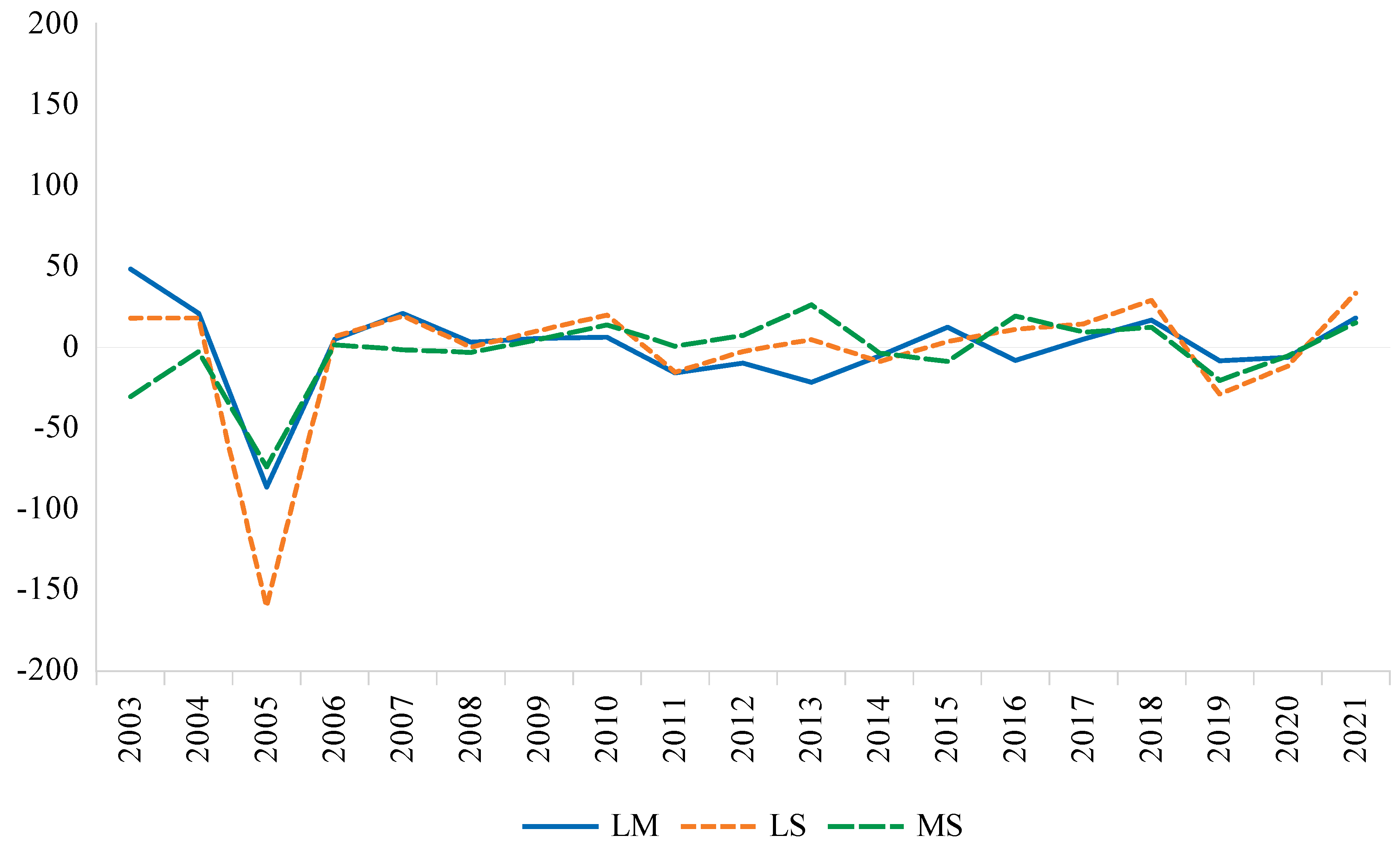
A visual inspection of Figure 1 clearly reveals the market bubble and spectacular market crash of 2006. Other notable events, such as the GFC, the 2014–2016 crude oil price plunge, the COVID-19 pandemic, and the Russo-Ukrainian war, are also evident. To focus on the relative performance of the size indices, we calculate the annual return spread between large- and mid-cap (ML), large- and small-cap (LS), and mid- and small-cap (MS) indices. According to the above definition of the annual return spread, a positive spread means that mid- and small-cap indices underperform their large-cap counterparts, while the opposite is true in the case of a negative spread. The obtained spreads, as depicted in Figure 2, reveal a few peaks and troughs over the sample period, although the trough around the 2006 market crash is the most pronounced. Before the bursting of the Saudi stock market bubble in 2006, small-cap stocks dramatically outperformed their large-cap counterparts by a considerable margin.
After the bursting of the 2006 bubble, the relative performance of large caps, as measured by the spread, seems to alternate dynamically between over- and underperformance relative to mid- and small caps, behavior that is largely in accordance with that documented by Jena et al. (2021) in the Indian market. Another inspection of Figure 2 reveals the extended period of large caps’ overperformance relative to small caps documented in the Saudi market by Katiyar and Dabake (2019) between 2016 and 2019.
The stochastic properties of the data were examined by means of descriptive statistics and preliminary tests that are reported in Table 1, which revealed that the mean of weekly returns for the large-cap index is the highest, followed by mid- and small-cap indices. The median, however, paints a different story, substantially exceeding the corresponding mean in all cases, suggesting a different order in terms of the magnitude of weekly returns, whereby the small-cap median return is higher than that of both mid- and large-cap indices, which is reflected by the negative skewness of the return distribution. The small-cap index exhibits the widest range and the highest standard deviation, reflecting the inherent volatility of small-cap companies. The mid- and large-cap indices, on the other hand, exhibit a narrower range and a lower standard deviation. Student’s t-statistics indicate that the mean of all indices is not significantly different from zero.
The excess kurtosis statistics are high, especially for the small-cap index, and the normality of the distribution of all the indices’ returns is rejected by the Jarque and Bera (1980) test for normality. Both the ADF (Dickey and Fuller 1981) and the PP (Phillips and Perron 1988) unit root tests reject the null hypothesis of a unit root for all indices, indicating that all return series that we consider are stationary. The Ljung–Box Q 4 test for (up to) fourth-order serial correlation shows that the returns of small- and mid-cap indices are serially correlated, while the returns of the large-cap index seem to be free from serial dependence. The Engle (1982) LM test’s null hypothesis of no ARCH effect up to order four is rejected for all indices, confirming the presence of conditional heteroscedasticity effects in all cases.
A salient feature of asset prices is the more pronounced impact of bad news on volatility compared to good news, which is referred to in the literature as the “leverage effect”. Engle and Ng (1993) proposed a diagnostic test for the presence of the leverage effect. The Engle–Ng sign bias test is conducted using the regression equation of the form
s t 2 = α 0 + α 1 d t 1 + α 2 d t 2 + α 3 d t 3 + e t
where s t is calculated from the residuals of a GARCH-type model1 as s t = ε ^ t / h ^ t 1 / 2 , while d t 1 is a dummy variable that is equal to 1 if ε ^ t 1 < 0 and is equal to zero if ε ^ t 1 0 , and e t is a regression residual. This test is used to ascertain whether the estimated squared residuals can be predicted using the d t 1 ,   d t 2 and d t 3 series. If the null hypothesis that H 0 : α 1 = 0 is rejected, then we can conclude that the sign of the current period shock is useful in predicting conditional volatility. To determine whether the magnitude of positive and negative shocks has an impact on their ability to predict conditional volatility, a more general form of the test is given by
s t 2 = β 0 + β 1 d t 1 + β 2 d t 1 s t 1 + β 3 ( 1 d t 1 ) s t 1 + e t
where d t 1 s t 1 and ( 1 d t 1 ) s t 1 indicate whether the effects of positive and negative shocks also depend on their size. A joint F-statistic is used to test the null hypothesis H 0 : α 1 = α 2 = α 3 = 0 and/or H 0 : β 1 = β 2 = β 3 = 0 . If the joint test is rejected, we can conclude that there is a leverage effect. The results of the Engle–Ng sign bias test are reported in Table 2.
Panel A of Table 2 reports the results of the Engle–Ng sign bias test based on the first test specification. The estimates of coefficient α 1 pertaining to the large- and small-cap indices are of the expected sign and are statistically significant at the 10% and 5% levels, respectively, while the coefficient pertaining to the mid-cap index is found to be insignificant. The positive sign on the coefficient α 1 indicates that negative values of s t 1 are associated with large values of s t 2 . The joint test results show that the null hypothesis H 0 : α 1 = α 2 = α 3 = 0 is rejected for large- and small-cap indices at the 10% and 5% levels, respectively, which indicates that the leverage effect is present in large- and small-cap indices but not in mid-cap stocks. The results in Panel B based on the general form of the bias test, which considers the magnitude of shocks in addition to their sign, yield stronger evidence in favor of the leverage effect. The joint test results show that null hypothesis H 0 : β 1 = β 2 = β 3 = 0 is rejected for all sized indices at least at the 10% level.
Moving to bivariate analysis, we examine unconditional correlations among the three different-sized portfolios as a precursor to multivariate GARCH modeling. The correlation matrix, as presented in Table 3, shows that the unconditional correlation coefficients between the three index sizes are large and positive. This implies that there is a strong link among large-, mid-, and small-cap indices and that they move in the same direction, on average. We also see that the lowest correlation coefficient is between large- and small-cap indices, reaching 0.71, while the correlations between large- and mid-caps, on the one hand, and between mid- and small-cap indices, on the other hand, are relatively high, reaching 0.84 and 0.85, respectively. While these findings indicate that small caps offer more diversification potential for large-cap portfolios, they should be interpreted with caution. The reason is that the Pearson correlation is linear and, thus, fails to account for potential nonlinear relations and time-varying linkages among these indices.

3.2. Methodology

The results emerging from the preceding section motivate the adoption of a GARCH-family model to explore the potential time-varying conditional correlation and volatility spillovers that may arise among large-, mid-, and small-cap indices. Bauwens et al. (2006) suggested that “the most obvious application of MGARCH (multivariate GARCH) models is the study of the relations between the volatilities and covolatilities of several markets”. Other applications of MGARCH models include the calculation of time-varying minimum variance hedge ratios and optimal portfolio weights (for example, Ahmad 2017; Akhtaruzzaman et al. 2021b; Klein et al. 2018).
While there are many MGARCH parametrizations, we decided to employ the Baba–Engle–Kraft–Kroner (BEKK) parametrization proposed by Engle and Kroner (1995) to examine the time-varying conditional correlation and volatility spillovers among large-, mid-, and small-cap indices. Our decision was based on the following reasoning: first, the BEKK parametrization avails itself of a broad range of interactions among the modeled series while ensuring positive definiteness of the conditional covariance matrix by construction; second, while it is true that the constant conditional correlation (CCC) proposed by Bollerslev (1990) is more parsimonious than the BEKK, “empirical studies have suggested that the assumption of constant conditional correlations may be too restrictive” (Silvennoinen and Teräsvirta 2009); third, Caporin and McAleer (2012) showed that the BEKK yields consistent estimates of dynamic conditional correlations and is preferred to the dynamic conditional correlation (DCC) proposed by Engle (2002) on theoretical grounds. On the basis of this argument, Boldanov et al. (2016) used BEKK and suggested that it may be better than DCC.
Given the above, we use an econometric specification that consists of two components, whereby a vector autoregression (VAR) is used to model the returns, while an asymmetric BEKK-GARCH model is used to model the time-varying variances and covariances. The VAR model accommodates autocorrelations and cross-autocorrelations in the returns’ series. The typical mathematical expression of a p-th order VAR model is written as
R t = Μ + Φ 1 R t 1 + Φ 2 R t 2 + + Φ p R t p + u t
where R t is a 3 × 1 vector containing the returns series of the three size-based stock portfolios in the VAR, Μ is a 3 × 1 vector of constant terms, Φ i is a 3 × 3 matrix for each lag p , and u t is a 3 × 1 vector of residuals. On the basis of Table A2 (in the Appendix A), we opted to proceed with a VAR model of order 1, denoted as VAR (1) and given by
R t = Μ + Φ 1 R t 1 + + u t
with
R t = r l , t r m , t r s , t ,   Μ = μ 1 μ 2 μ 3 ,   Φ 1 = ϕ 11 ϕ 12 ϕ 13 ϕ 21 ϕ 22 ϕ 23 ϕ 31 ϕ 32 ϕ 33 , u t = u l , t u m , t u s , t
where the diagonal elements of matrix Φ 1 , namely, ϕ 11 , ϕ 22 , and ϕ 33 , represent the first-order autoregressive coefficients, while the off-diagonal elements capture the mean spillovers among the three portfolios. Here, the residuals u t are normally distributed, given the information available at time t 1 denoted as I t 1 , as u t | I t 1 ~ N 0 , H t with a zero mean and a conditional variance–covariance matrix modeled using a BEKK-GARCH (1, 1) specification as follows:
H t = C C ´ + A ´ u t u t ´ A + B ´ H t B
where C is a lower triangular matrix of the constant term, and A and B are general 3 × 3 matrices. On the basis of the results of the Engle–Ng sign bias test in Section 2.1, we add asymmetry to the BEKK model such that the model is rewritten as
H t = C C ´ + A ´ u t u t ´ A + B ´ H t B + D ´ v t v t ´ D
The dimensions of matrix D are the same as the matrices of A and B , and v t is the adjustment for asymmetry that is defined as v t = u t if u t < 0 (i.e., negative shock) and v t = 0 otherwise.
With
H t = h 11 , t h 12 , t h 13 , t h 21 , t h 22 , t h 23 , t h 31 , t h 32 , t h 33 , t , C = c 11 0 0 c 21 c 22 0 c 31 c 32 c 33 , A = a 11 a 12 a 13 a 21 a 22 a 23 a 31 a 32 a 33 , B = b 11 b 12 b 13 b 21 b 22 b 23 b 31 b 32 b 33 , D = d 11 d 12 d 13 d 21 d 22 d 23 d 31 d 32 d 33 , v t = v l , t v m , t v s , t
where h 11 , t , h 22 , t , h 33 , t within the conditional variance–covariance matrix, H t , are the conditional variances of the large, mid, and small portfolios, respectively, while h i j , t     i j are the conditional covariance of each pair of size-based portfolios i and j . Matrix A contains the ARCH coefficients, whereby the diagonal elements a 11 , a 22 , a 33 represent the own ARCH effect of the fluctuations of the three portfolios, representing the short-run persistence of shocks, whereas the off-diagonal elements represent the cross-shock spillover among the three portfolios. Matrix B contains the GARCH coefficients of the model, where the diagonal elements b 11 , b 22 , b 33 are the own GARCH effect of the three portfolios, representing the long-run persistence of volatilities in each portfolio, while the off-diagonal elements represent the volatility spillover effects among the three portfolios. D is a matrix of coefficients that capture asymmetric responses to shocks where the diagonal elements d 11 , d 22 , d 33 represent the own-asymmetric shock spillovers, whereas off-diagonal elements represent the cross-asymmetric shock spillovers.
Indeed, GARCH-family models assume that the modeled series is generated by a single GARCH process over the entire sample period. However, several studies have shown that structural breaks are prevalent in financial time series (for example, Andreou and Ghysels 2002; James Chu 1995; Dieobold 1986). Lastrapes (1989) and Lamoureux and Lastrapes (1990) suggested that the presence of structural shifts may undermine the volatility models’ estimation of persistence, displaying higher persistence in volatility than what is, in fact, the case. Ewing and Malik (2005) found that ignoring structural shifts can potentially lead to an overestimation of the degree of volatility spillovers among the modeled series, while Halunga and Savva (2019) indicated that ignoring these shifts can ultimately confound portfolio and risk management decisions. To guard against this problem, we use the Nyblom (1989) stability test. If the null of a stable model is rejected, we include shift dummies in the variance equation.

4. Empirical Results

4.1. Regression Estimation Results and Their Interpretation

This section reports and discusses the estimation results of the asymmetric VAR-BEKK-GARCH (1,1) model. The model is estimated by quasi maximum likelihood estimation (QMLE), where the simplex algorithm is used to obtain the initial conditions by running several iterations. Subsequently, the final estimate of the variance–covariance matrix is obtained by means of the BFGS algorithm. The t-distribution and robust standard errors are used2. The VAR-BEKK-GARCH (1,1) model’s parameter estimates and diagnostic tests are reported in Table 4 and Table 5, respectively. Before we interpret the parameter estimates, an examination of the diagnostic tests is warranted. On the basis of Table 5, we find that, while the tests for the standardized residuals and standardized residuals squared show no evidence of serial correlation at the 5% significance level, Nyblom’s joint test is rejected at the same level of significance. The rejection of Nyblom’s joint test indicates that there is sufficient evidence to conclude that the VAR-BEKK-GARCH (1,1) model’s parameters are jointly not stable. Therefore, we include shift dummies in the variance equation to control for the potential shifts in the variance, and the results are reported in Table 4 and Table 5 next to those of VAR-BEKK-GARCH (1,1)3. The results pertaining to the BEKK model with shift dummies in Table 5 demonstrate that there is no sufficient evidence to reject Nyblom’s joint test, which indicates that the parameters of the VAR-BEKK-GARCH (1,1) model with shift dummies are jointly stable.
Now, we proceed to the interpretation of the parameter estimates in Table 4. We start with the VAR (1) model for returns. The most conspicuous finding is that the returns of small-cap stocks are positively affected by the first lagged returns of their mid-cap counterparts. The estimated parameter of the mid-cap index in the small-cap equation ( ϕ 32 ) is positive and significant at the 1% level for both models, confirming the presence of significant unilateral mean spillovers from mid- to small-cap stocks. Because we include more than two series in our models, the use of the joint Wald test is more convincing, as it accounts for the effect of indirect shocks. For example, shocks to the first series can possibly affect the third series indirectly via the second series if a shock to the first affects the second series directly. The results of the block exclusion tests for the first and second models are reported in Table 6 and Table 7, respectively. The results pertaining to the mean equation in Table 6 show that the null hypothesis of exogeneity is rejected at the 5% level, confirming the presence of spillovers/causality among the three different-sized portfolios, which is also supported by the second model in Table 7, albeit only at the marginal 10% level. To dig deeper into the direction of spillovers/causality, the null hypothesis of exogeneity is also tested with respect to each size portfolio. Remarkably, evidence in favor of rejecting the null of exogeneity is only found for the small-cap portfolio at the 5% level across both models, which means that there is unilateral causality running from larger caps (mainly from mid-caps) to the small-cap portfolio, which is largely consistent with the findings of early studies, for example, Lo and MacKinlay (1990b) and Chelley-Steeley and Steeley (1996), in addition to more recent studies including Marshall and Walker (2002) and Drakos (2016), in confirming the presence asymmetric lead–lag relation in returns. The stronger linkages between small- and mid-caps, in particular, are in accordance with the evidence obtained by Mills and Jordanov (2001), who showed that portfolio-specific shocks affect firms of similar size more than firms of substantially different size. This spillover effect, indeed, casts doubt on the pricing efficiency of small caps.
Next, we turn to the parameter estimates of the ARCH and GARCH terms in Table 4. The estimates of the diagonal elements of matrix A , i.e., a 11 , a 22 , and a 33 (ARCH effects), measure the short-term persistence of the own past shocks, whereas those of matrix B , i.e., b 11 , b 22 , and b 33 (GARCH effects), measure the long-term persistence of own volatility. We can clearly see that own ARCH effects ( a 11 , a 22 , and a 33 ) are of similar magnitude across both models, showing significance at the 1% level, which implies that each of the three different-sized portfolios is impacted by its own past shocks. A similar pattern is observed for the own GARCH effects ( b 11 , b 22 and b 33 ), which are also found to be of similar magnitude, displaying significance at the 1% level across both models, which means that each size portfolio is influenced by its own volatility. For each of the portfolios, the values of the estimated own ARCH parameters a 11 , a 22 , and a 33 are smaller than their corresponding GARCH counterparts, namely, b 11 , b 22 , and b 33 . That is, past volatilities are more important than shocks in predicting future volatility, which is in line with results reported elsewhere.
Notwithstanding the significance of the own ARCH and GARCH effects in predicting future volatility, shock and volatility spillovers among the three portfolios are also crucial. Therefore, we consider the parameter estimates of the off-diagonal elements of matrix A i.e., a i j     i j , and matrix B , i.e., b i j     i j , which capture the linkages among the three portfolios in the form of shock and volatility spillovers between these portfolios, respectively. While the results pertaining to the own ARCH and GARCH effects are consistent across the two models, several disparities are evident when considering the spillover effects. As we move to the BEKK model with the shift dummies, the spillover effects become weaker.
On the basis of the results pertaining to the ARCH spillover effects, only in one instance are the two models consistent in documenting a significant spillover parameter ( a 32 ) that is of the same magnitude and shows significance at the 1% level. The interpretation of this parameter is that short-term shocks originating in the small-cap portfolio increase the volatility of the mid-cap portfolio in the short run, but the opposite effect does not hold, as a 23 is not significant. The remaining parameter estimates of the off-diagonal elements of matrix A are consistent across the two models and are statistically insignificant, except for a 21 , which is strongly significant at the 1% level when considering the first model only but loses significance when the second model is used.
The results pertaining to GARCH spillover effects as represented by the parameter estimates of the off-diagonal elements of matrix B paint a similar picture. Three of the six GARCH spillover parameters, namely, b 12 , b 13 , and b 31 (which are significant at the 1% level when the first model is used), lose their significance when the second model is considered. Two of the remaining three parameters, namely, b 21 and b 23 (which are significant at the 1% level when the first model is used), become marginally significant at the 10% level according to the second model. The parameter b 32 that is found to be statistically insignificant is the only GARCH spillover parameter showing consistency across the two models. A word on the interpretation of the parameters b 21 and b 23 is warranted. The negative sign on b 21 and b 23 indicates that long-term volatility originating in the mid-cap portfolio has a calming effect on the volatility of the large- and small-cap portfolios.
We move on to the bottom of Table 4 to consider the asymmetric volatility spillover effects measured by the parameter estimates of the elements of matrix D . The diagonal elements of matrix D , i.e., d 11 , d 22 and d 33 , which measure the asymmetric own shocks to returns, are mixed across the three portfolios. The estimates of d 11 ( d 33 ) are consistently positive (negative) and significant at the 1% level for both models, which means that bad news (i.e., negative shocks) amplifies (diminishes) the volatility of the large-cap (small-cap) portfolio to a greater extent than good news does. The estimates of d 22 are, however, marginally significant at the 10% level and lose significance when we consider the second model, which is indicative of the weakness of the asymmetric own shocks’ effect on the mid-cap portfolio’s volatility.
Regarding the estimates of the off-diagonal elements of matrix D , i.e., d i j = 0     i   &   j , we also find significant asymmetric volatility spillover effects among the three portfolios. When considering large and small caps, the effects are largely consistent across the two models in terms of the sign, magnitude, and significance at the 1% level (except for d 31 in the second model), although these portfolios display the opposite sign. The positive sign of the estimates of parameters d 12 and d 13 means that bad news from the large-cap portfolio increases the variability of mid- and small-cap returns. In contrast, the parameter estimates of d 31 and d 32 have a negative sign, implying that bad news from the small-cap portfolio decreases the variability of large- and mid-cap returns. Lastly, the parameter estimates pertaining to the mid-cap portfolio, d 21 and d 23 , become statistically insignificant when using the second model, implying diminished evidence for asymmetric volatility spillover from the mid-cap portfolio when the second model is considered.
Now, we move to the joint Wald test results pertaining to the variance equation in Table 6 and Table 7 to examine whether any form of variance spillover is present. The block exclusion test applied to the off-diagonal elements of matrices A and B strongly rejects the null of diagonality at the 1% level. To tease out the nature of the variance spillovers among the three size portfolios, the null of diagonality is also tested for each portfolio. Table 6 and Table 7 clearly show that the results obtained using the first model, as presented in Table 6, support the presence of multilateral spillovers across the three different-sized portfolios, at least at the 10% level. However, on the basis of Table 7, spillovers are generally weakened when we consider the second model. Only in the case of mid-caps did the spillovers from large and small caps remain significant, albeit at the marginal level of 10%, which is in line with the findings of Ewing and Malik (2005) and Marcelo et al. (2008). This outcome emphasizes the importance of accounting for market crises which affect the volatility transmission mechanism. Lastly, the null of symmetric behavior is strongly rejected across the two models, reinforcing the importance of accounting for asymmetry.

4.2. Time-Varying Conditional Correlation

The time-varying conditional correlation among large-, mid-, and small-cap portfolios’ return volatility can be calculated using the estimated conditional variance–covariance matrix, H t , of the two VAR-BEKK-GARCH (1,1) models as follows:
ρ i j , t = h i j , t h i i , t h j j , t
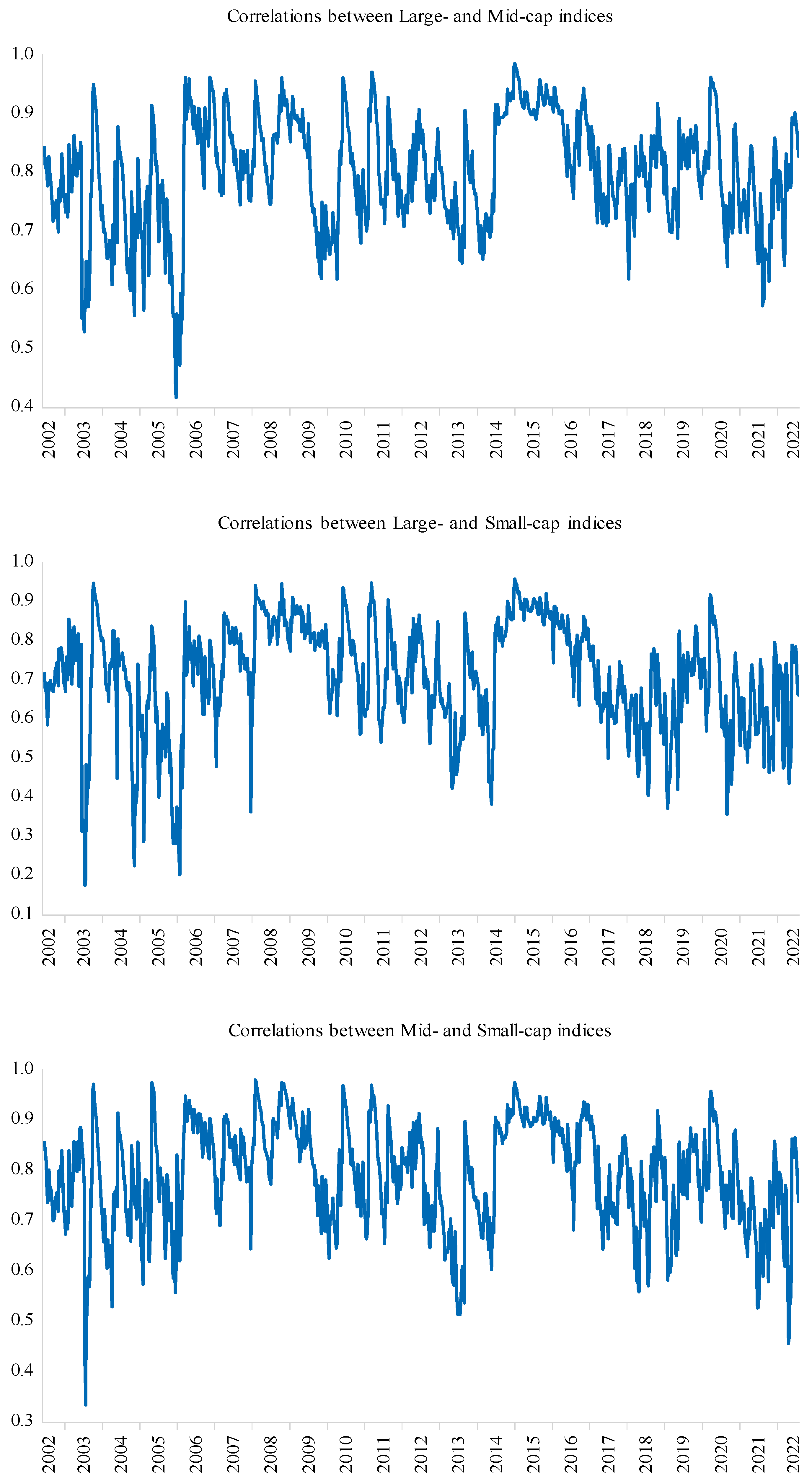
Figure 3 presents the time-varying conditional correlations4. An important realization gleaned from Figure 3 is that the time-varying conditional correlations can depart significantly from the estimated unconditional correlations in Table 3, which emphasizes the inadequacy of unconditional correlations in capturing the correlation dynamics. We observe that large, mid, and small caps have a strong positive correlation with one another, although it fluctuates over a wide range. Remarkably, correlations between large- and small-cap indices range from as low as 0.17 to as high as 0.96. However, the range within which correlations fluctuate narrowed after the GFC as the Saudi stock market became more mature. In all cases, we observe that correlation peaks during the periods of market turmoil that coincide with major events, including the bursting of the Saudi stock market bubble in 2006, the GFC, the collapse of oil prices in 2014, the COVID-19 outbreak, and the Russo-Ukrainian war. Thus, we are led to believe that calculations based on unconditional correlation would have led to erroneous hedging and portfolio allocation decisions.

5. Portfolio and Risk Management Implications

The estimated conditional variance–covariance matrix obtained in the preceding sections is used to extract valuable insights that guide two of the most essential tasks performed by finance professionals: allocation of funds to potential investments, and hedging strategies that are employed to mitigate market risk associated with investing in volatile assets.

5.1. Fund Allocation

The documented volatility spillovers among the three different-sized portfolios warrant a careful analysis of fund allocation decisions over the period of our study. Such an exercise may shed light on the impact of several crises (including the 2006 bubble, GFC, 2014–2016 crude oil price plunge, COVID-19, and the Russo-Ukrainian war) on investors’ asset allocation decisions, thereby conveying our econometric results to practitioners’ intuition.
This can be achieved by means of the widely used Kroner and Ng (1998) approach that constructs a portfolio by calculating the weights allocated to the portfolio constituents such that the portfolio’s risk is minimized without reducing its expected returns. The inputs required to compute the optimal weights are obtained from the estimated conditional variance–covariance matrix, H t , for our two VAR-BEKK-GARCH (1,1) models. The optimal weight of the first size-based index i in a one-dollar portfolio that consists of two different-sized indices i and j at time t is given by
w i j , t = h j j , t h i j , t h i i , t 2 h i j , t + h j j , t
A routine assumption that is usually made in this context is
w i j , t = 0   i f   w i j , t < 0   w i j , t   i f   0 w i j , t 1   1   i f   w i j , t > 1  
where w i j , t is the weight of the first size-based index i in a one-dollar portfolio of the two different-sized indices i and j at time t , the term h j j , t is the conditional variance of index j at time t , h i j , t is the conditional covariance between the two different-sized indices i and j at time t, and h i i , t is the conditional variance of index i at time t . By definition, the weight of index j in this portfolio is 1 w i j , t .
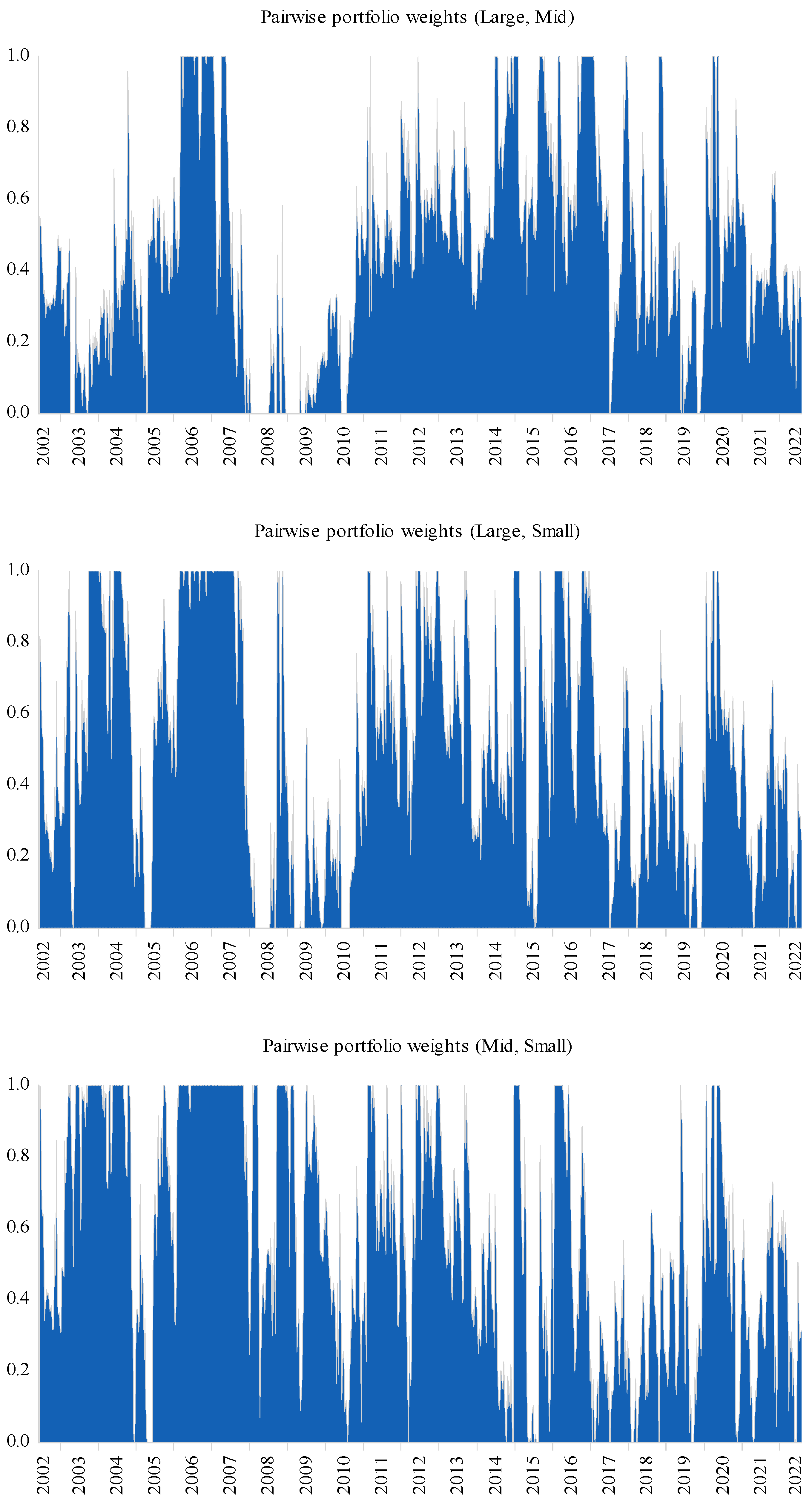
Table 8 reports the optimal weight results. From Panel A of Table 8, which pertains to the first model, we see that portfolio L/M, which combines the large- and mid-cap stocks, has a mean weight of 0.46. This implies that for a USD 1 portfolio, 46 cents should be allocated to large caps, while the remaining funds, i.e., 54 cents, should be used to invest in mid-caps. The mean weight for portfolio L/S, which includes the large- and small-cap stocks, is 0.51, which means that the funds allocated to large caps exceed those allocated to small caps by only 1 cent. The mean of portfolio M/S, which includes the mid- and small-cap stocks, confirms that mid-caps acquire the lion’s share of fund allocation when either combined with large or small caps; in this case, 57 cents are invested in mid-caps, and the remaining 43 cents go to small caps. To complete our understanding, we examine the standard deviations of the weights, which are quite large, reaching 0.29, 0.33, and 0.32 for the L/M, L/S, and M/S portfolios, respectively. Additionally, according to the min and max results for all portfolios, we see that in some instances, the fund allocation to any of the three portfolio constituents ranges from as high as 100% of the funds to as low as 0%. Interestingly, the results obtained from the second model, as presented in Panel B of Table 8, are nearly identical to those of the first model. Because of the high dispersion of the estimated weights, we plot the dynamic weights in Figure 4 to depict how portfolio allocation changes over time5.
Figure 4 clearly reveals, in all cases, that the portfolio weights are not stable, indicating that investors dynamically change their allocations to different capitalizations over time. Considering portfolio L/M, we see that more weight is allocated to large caps during turbulent time periods, with the entire portfolio being solely invested in large caps (i.e., w L M , t = 1 ) in many instances. The same is true and even more pronounced for portfolios L/S and L/M, indicating a flight to quality from smaller to larger capitalizations. Indeed, one clear exception is that allocation to large against mid-caps reached zero (i.e., w L M , t = 0 ) for extended time periods during the GFC. This can be explained by the fact that the large-cap index is dominated by the banking and petrochemical sectors that were more exposed to the ramifications of the GFC.

5.2. Hedge Ratios

As for the optimal weight in the preceding section, hedging decisions in this study are based on the estimated conditional variance–covariance matrix. To determine the size of our hedging positions, we rely on the widely used Kroner and Sultan (1993) approach, which specifies the size of the hedging position by means of the optimal hedge ratio. To derive the optimal hedge ratio, Kroner and Sultan (1993) consider a portfolio comprising two assets and postulate that the risk of this portfolio is minimized when the long position of one dollar in the first asset is hedged by shorting β t dollars of the second asset. The optimal hedge ratio between any two size-based indices is given by
β i j , t = h i j , t h j j , t  
Here, a long position of one dollar in the first size-based index i is hedged by a short position of size β i j , t dollars in the second size-based index j to minimize the portfolio risk.
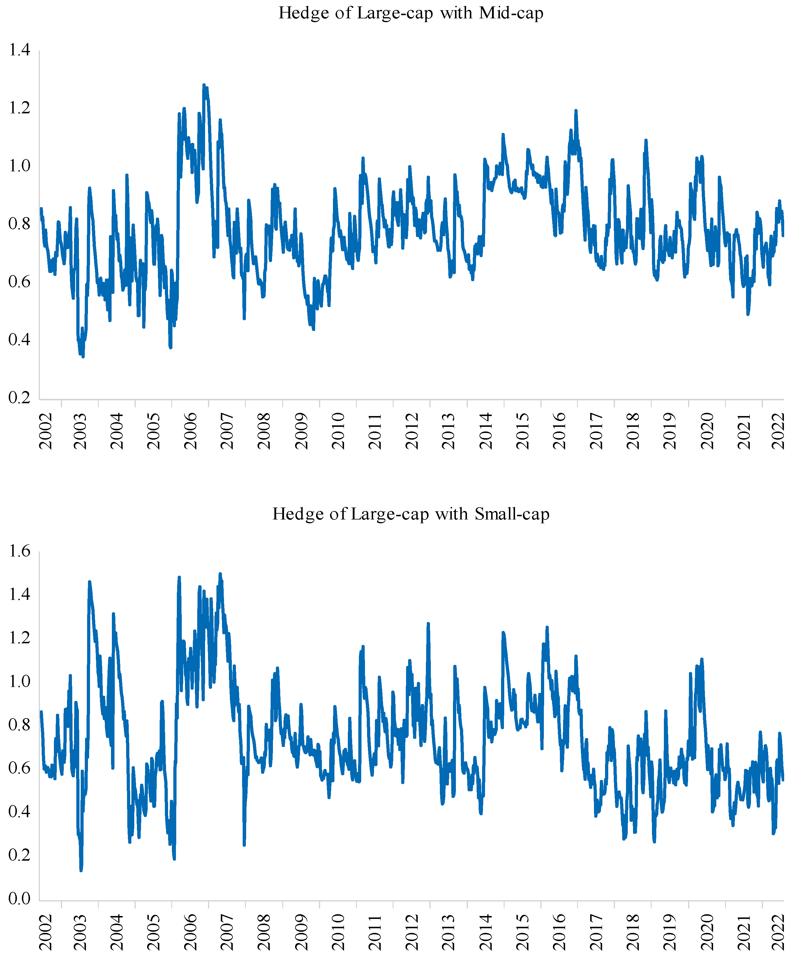
Table 9 reports the optimal hedge ratio results. Panel A of Table 9, which pertains to the first model, shows that the mean value of the hedge ratio between large and mid-caps (L/M) is 0.79, while the mean value of the hedge ratio between large and small caps (L/S) is slightly lower at 0.75. The highest hedge ratio is recorded between mid- and small caps (M/S), reaching a mean value of 0.85. These results mean that a long position of USD 1 in large caps can be hedged with a short position of 79 (75) cents in mid- (small) caps. On the other hand, a USD 1 long position in mid-caps can be hedged by opening a short position of 85 cents in small caps. Indeed, the standard deviation of the hedge ratios indicates that optimal hedging positions fluctuate considerably, as can also be seen considering the min and max values. In accordance with the findings pertaining to portfolio weights, the results presented in Panel B of Table 9, which were generated on the basis of the second model, bear a strong resemblance to those of the first model.
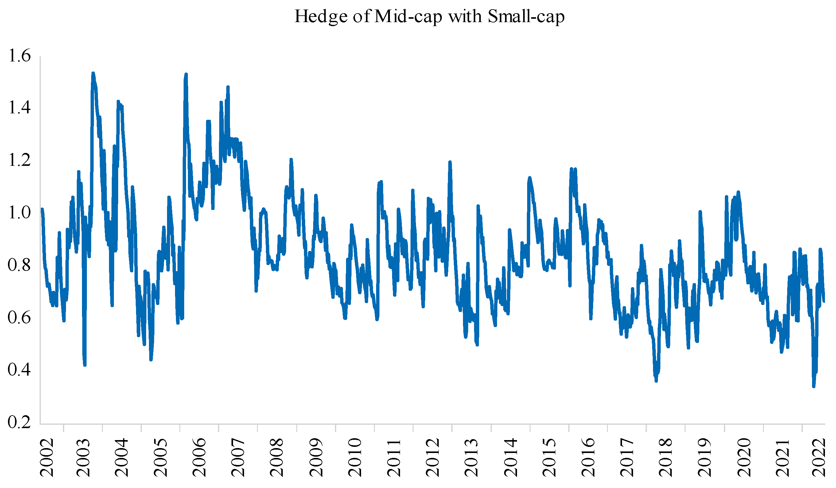
Because of the high dispersion of the estimated hedge ratios, we plot the dynamic hedge ratios, as presented in Figure 5, to examine how hedging positions change over time6. From Figure 5, we see that the hedge ratios vary over time, exhibiting values greater than one during turbulent periods. This means that a hedger faces higher hedging costs due to the need to take a larger position to short the corresponding capitalization index during uncertain times which align with findings of previous studies, for example, Akhtaruzzaman et al. (2021a) and Mensi et al. (2021).

6. Robustness Check

As an alternative approach, we employ the Dieobold and Yilmaz approach for spillover measurement7. This approach enables us to gauge static and time-varying volatility connectedness among the different-sized portfolios. The results of the static volatility connectedness are reported in Table 10. A look at the lower right corner of Table 10 reveals that about half (50.96%) of the volatility of the forecast error variance in all three portfolios originates from spillovers. Our estimate falls between those reported in Apostolakis et al. (2021) (42.80%) for the Greek market and Jena et al. (2021) (59.93%) for the Indian market.
Interestingly, the mid-cap portfolio transmits more volatility than it receives from large- and small size portfolios, emerging as a net contributor of volatility to the system which is consistent with Jena et al. (2021). On the other hand, large- and small-sized portfolios turn out to be net receivers of volatility spillovers.
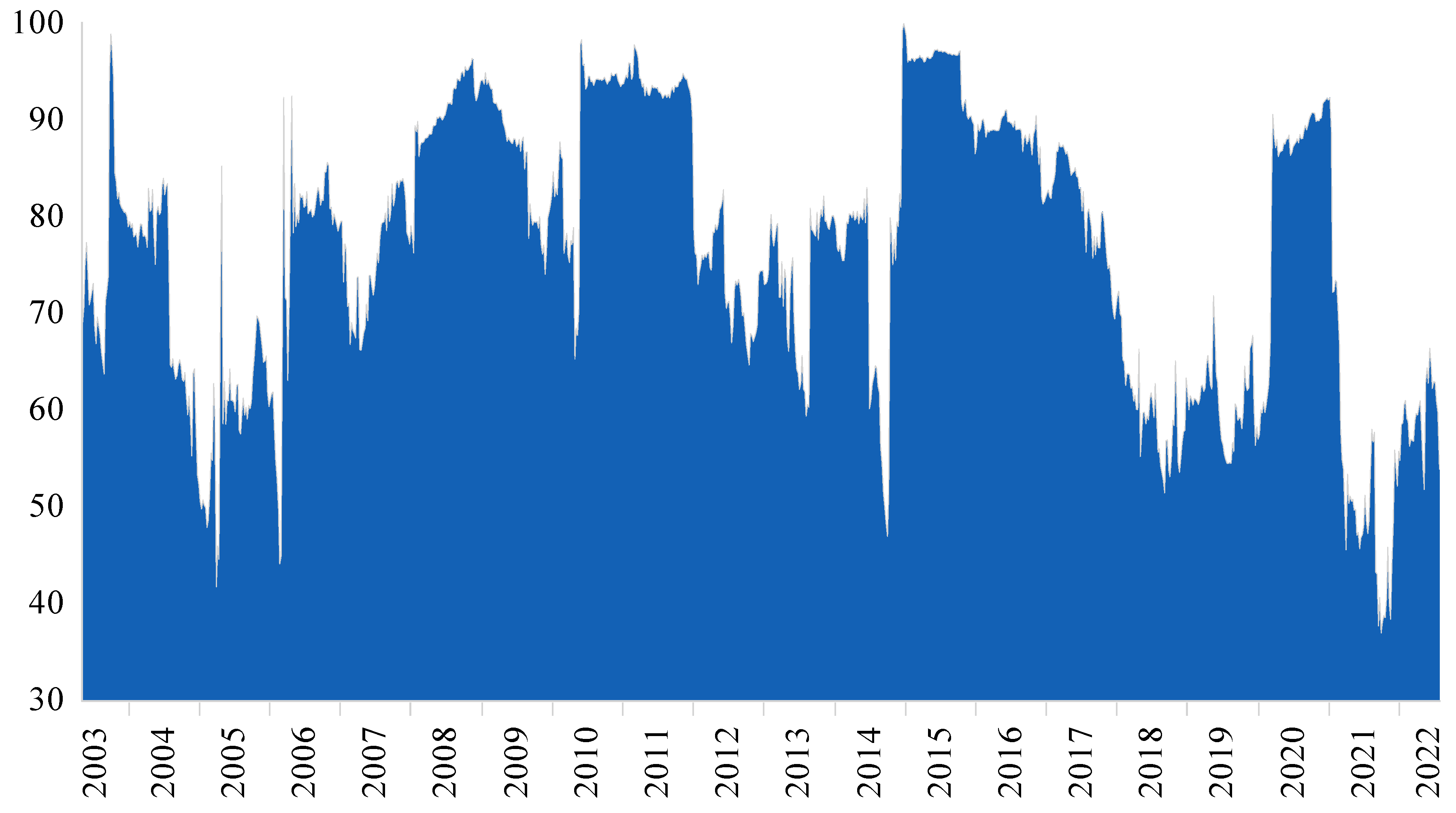
Notwithstanding the valuable insights that we obtained from static analysis of spillover; it is merely an average description of the system. A more detailed look at the evolution of spillovers dynamics over the sample period can be achieved by the means of a rolling-sample total connectedness plot constructed on the basis of a 52-week rolling widow. The results are depicted in Figure 6. From Figure 6, we can clearly see spikes in total connectedness corresponding to the major financial/economic crises, including the bursting of the Saudi stock market bubble in 2006, GFC, the 2014–2016 crude oil price plunge, the COVID-19 pandemic, and the Russo-Ukrainian war. Indeed, the Russo-Ukrainian war induced volatility connectedness is mild compared to the other crises. These findings are concurrent with those of the BEKK-GARCH model.
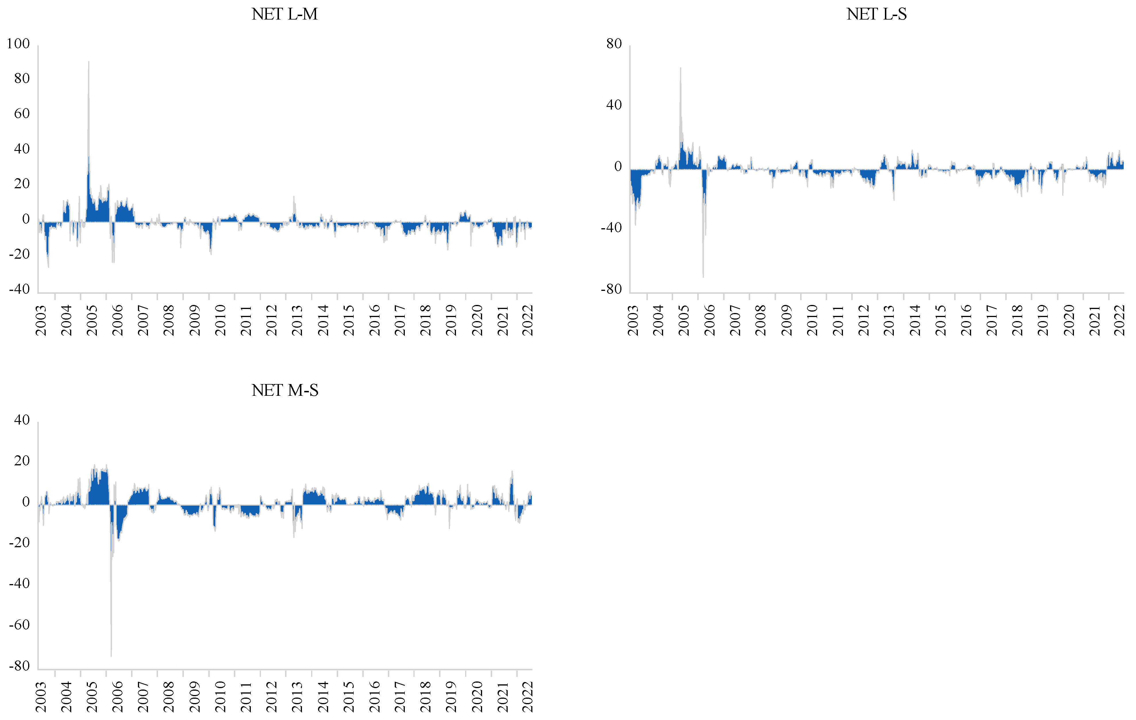
To obtain a refined insight on the bilateral volatility connectedness, we estimate the net pairwise connectedness on the basis of a 52-week rolling widow and present the results in Figure 7.
Figure 7 shows that all three portfolios oscillate between net receivers and net transmitters of volatility shocks. A remarkable observation is the sharp downward spike in the midst of the 2006 Saudi stock market crash. The net pairwise connectedness, presented by the NET L/S and NET M/S graphs, within Figure 7 clearly shows that small caps emerge as net transmitter of volatility shocks to their large- and mid-cap counterparts. This finding highlights the role that small caps assume as sources of volatility during that period. This can be explained by the excessive speculation on the small caps that inflated their prices which later reverted back to closer to their fundamental values. This finding is in sync with the results obtained from portfolio analysis, which indicates that investors drastically underweighted small caps in their portfolios.

7. Discussion and Conclusions

The size effect is one of the mainstays of the finance literature. This effect transcended academic circles to the finance industry, manifesting itself via size-based stock market indices and investment styles. Despite the controversies raised by its critics, the size effect apparently stood the test of time. A careful examination of the linkages among small- and large-cap portfolios and their associated portfolio management implications is a natural extension to this literature. We take a step in this direction to gain fresh insight by examining the return and volatility spillovers and time-varying conditional correlations among large-, mid-, and small-cap indices and their portfolio allocation and risk management implications in the context of the Saudi market, the leading market in the Middle East. To do so, we estimate a VAR-asymmetric BEKK-GARCH model while accounting for structural breaks using a long sample period spanning the most substantial market crises in the past two decades.
The empirical results show, on the one hand, that there exist unilateral return spillovers running from mid- to small-cap stocks, implying that mid-cap portfolio returns can predict future small-cap returns, but not vice versa, which casts doubts on the pricing efficiency of small caps and corroborates the traditional asymmetric lead–lag relation. On the other hand, multilateral volatility spillover effects are documented among the three different-sized portfolios. However, when structural breaks are carefully modeled, the spillovers are substantially weakened, remaining evident, particularly among mid- and small caps. This spillover pattern potentially drives the transfer of information via rebalancing portfolios that comprise mid- and small caps rather that large-cap portfolios that are more likely to be passively managed. The time-varying conditional correlations intensify around crisis periods, leading to higher hedge ratios, which makes hedging during turbulent times more expensive. However, the intensity of the jumps in conditional correlations vary across different crises with the Russo-Ukraine war having a lower effect relative to previous crises. This is in line with the findings of Boubaker et al. (2022) who showed that the Middle Eastern stock markets reacted positively to the war news. The optimal portfolio weights suggest that investors generally overweight larger caps in their portfolios during uncertain times to minimize the risk of their portfolios without reducing their corresponding expected returns. However, the impact of the GFC on asset allocation differs from that of other crises. A plausible explanation is perhaps that the large-cap index is dominated by the banking and petrochemical sectors that were more exposed to the ramifications of the GFC.
The main takeaway from our results is that passively confining fund managers to a particular size category regardless of the prevailing market conditions may lead to suboptimal performance. Our findings are relevant for fund managers who are exposed to the Saudi market. We believe that extending this research to different investment styles other than market capitalization by using alternative statistical techniques, such as correlation networks (see, for example, Giudici and Polinesi 2021), is a promising research avenue.

Funding

This research received no external funding.

Informed Consent Statement

Not applicable.

Data Availability Statement

The data used is this study was obtained from Refinitiv DataStream and can be made available upon request from the corresponding author with the permission of Refinitiv.

Conflicts of Interest

The author declares no conflict of interest.

Appendix A

Table A1. The parameters of the univariate GARCH model.
ω α β α + β Half LifeLL
Large0.740.270.710.97730.12−2652.441
[0.00][0.00][0.00]
Mid0.860.330.650.98339.46−2610.8265
[0.00][0.00][0.00]
Small0.660.280.721.00 −2668.8324
[0.00][0.00][0.00]
Notes: The mean and variance equations are specified as r t = μ + ε t and h t = ω + α ε t 1 2 + β h t 1 , respectively. For the small-cap index, we estimate an IGARCH model; p-values are presented in square brackets.
Table A2. Lag order selection criteria.
Lag OrderAICSCHQ
014.5153114.52950 *14.52069
114.4838814.5406514.50541 *
214.4963414.5957014.53402
314.45710 *14.5990414.51092
414.4631214.6476414.53309
Notes: AIC is the Akaike information criterion, SC is the Schwarz information criterion, and HQ is the Hannan–Quinn information criterion. * indicates lag order selected by the criterion.

Notes

1
The estimation results of the GARCH model used to obtain the residuals on the basis of which the s t 2 is calculated are relegated to the Appendix A (Table A1) to conserve space.
2
The student distribution is used because the return series for small mid- and large caps do not follow the normal distribution (see Fiorentini et al. 2003).
3
On the basis of Nyblom’s individual test statistics, the endogenously determined shift dummies coincide with bursting of the Saudi stock market bubble in 2006, the GFC, and the 2014–2016 crude oil price plunge. The first dummy spans the period from 21 February 2006 to 18 August 2009, while the second dummy falls between 17 June 2014 and 29 December 2015.
4
The time-varying conditional correlations are based on the BEKK model with shift dummies. The time-varying conditional correlation values for the first model are not reported for the sake of brevity, but the corresponding author will make them available upon reasonable request.
5
The dynamic weights are based on the BEKK model with shift dummies. The dynamic weights for the first model are not reported for the sake of brevity, but the corresponding author will make them available upon reasonable request.
6
The dynamic hedge ratios are based on the BEKK model with shift dummies. The dynamic hedge ratios for the first model are not reported for the sake of brevity, but the corresponding author will make them available upon reasonable request.
7
To conserve space, we did not include a self-contained description of the model. For a comprehensive description of this methodology, see Dieobold and Yilmaz (2012).

References

  1. Abakah, Emmanuel Joel Aikins, Aviral Kumar Tiwari, Imhotep Paul Alagidede, and Shawkat Hammoudeh. 2023. Nonlinearity in the causality and systemic risk spillover between the OPEC oil and GCC equity markets: A pre- and post-financial crisis analysis. Empirical Economics 65: 1027–103. [Google Scholar] [CrossRef]
  2. Abuzayed, Bana, and Nedal Al-Fayoumi. 2021. Risk spillover from crude oil prices to GCC stock market returns: New evidence during the COVID-19 outbreak. The North American Journal of Economics and Finance 58: 101476. [Google Scholar] [CrossRef]
  3. Ahmad, Wasim. 2017. On the dynamic dependence and investment performance of crude oil and clean energy stocks. Research in International Business and Finance 42: 376–89. [Google Scholar] [CrossRef]
  4. Akhtaruzzaman, Md, Sabri Boubaker, and Ahmet Sensoy. 2021a. Financial contagion during COVID-19 crisis. Finance Research Letters 38: 101604. [Google Scholar] [CrossRef]
  5. Akhtaruzzaman, Md, Sabri Boubaker, Brian M. Lucey, and Ahmet Sensoy. 2021b. Is gold a hedge or a safe-haven asset in the COVID-19 crisis? Economic Modelling 102: 105588. [Google Scholar] [CrossRef]
  6. Al-Nassar, Nassar S., and Beljid Makram. 2022. The COVID-19 Outbreak and Risk–Return Spillovers between Main and SME Stock Markets in the MENA Region. International Journal of Financial Studies 10: 6. [Google Scholar] [CrossRef]
  7. Al-Nassar, Nassar S., Sabri Boubaker, Anis Chaibi, and Beljid Makram. 2022. In search of hedges and safe havens during the COVID-19 pandemic: Gold versus Bitcoin, oil, and oil uncertainty. The Quarterly Review of Economics and Finance 90: 318–32. [Google Scholar] [CrossRef]
  8. Alotaibi, Abdullah R., and Anil V. Mishra. 2017. Time varying international financial integration for GCC stock markets. The Quarterly Review of Economics and Finance 63: 66–78. [Google Scholar] [CrossRef]
  9. Al-Rodhan, Khalid R. 2005. The Saudi and Gulf Stock Markets: Irrational Exuberance or Markets Efficiency. Washington, DC: Center for Strategic and International Studies CSIS. Available online: https://www.csis.org/analysis/saudi-and-gulf-stock-markets-irrational-exuberance-or-markets-efficiency (accessed on 19 June 2022).
  10. Al-Yahyaee, Khamis Hamed, Walid Mensi, Ahmet Sensoy, and Sang Hoon Kang. 2019. Energy, precious metals, and GCC stock markets: Is there any risk spillover? Pacific-Basin Finance Journal 56: 45–70. [Google Scholar] [CrossRef]
  11. Andreou, Elena, and Eric Ghysels. 2002. Detecting multiple breaks in financial market volatility dynamics. Journal of Applied Econometrics 17: 579–600. [Google Scholar] [CrossRef]
  12. Apostolakis, George N., Christos Floros, Konstantinos Gkillas, and Mark Wohar. 2021. Political uncertainty, COVID-19 pandemic and stock market volatility transmission. Journal of International Financial Markets, Institutions and Money 74: 101383. [Google Scholar] [CrossRef]
  13. Arouri, Mohamed El Hedi, Amine Lahiani, and Duc Khuong Nguyen. 2011. Return and volatility transmission between world oil prices and stock markets of the GCC countries. Economic Modelling 28: 1815–25. [Google Scholar] [CrossRef]
  14. Asness, Clifford, Andrea Frazzini, Ronen Israel, Tobias J. Moskowitz, and Lasse H. Pedersen. 2018. Size matters, if you control your junk. Journal of Financial Economics 129: 479–509. [Google Scholar] [CrossRef]
  15. Awartani, Basel, and Aktham Issa Maghyereh. 2013. Dynamic spillovers between oil and stock markets in the Gulf Cooperation Council Countries. Energy Economics 36: 28–42. [Google Scholar] [CrossRef]
  16. Badrinath, Swaminathan G., Jayant R. Kale, and Thomas H. Noe. 1995. Of Shepherds, Sheep, and the Cross-autocorrelations in Equity Returns. The Review of Financial Studies 8: 401–30. [Google Scholar] [CrossRef]
  17. Balcilar, Mehmet, Ahmed H. Elsayed, and Shawkat Hammoudeh. 2023. Financial connectedness and risk transmission among MENA countries: Evidence from connectedness network and clustering analysis1. Journal of International Financial Markets, Institutions and Money 82: 101656. [Google Scholar] [CrossRef]
  18. Balcılar, Mehmet, Rıza Demirer, and Shawkat Hammoudeh. 2015. Regional and global spillovers and diversification opportunities in the GCC equity sectors. Emerging Markets Review 24: 160–87. [Google Scholar] [CrossRef]
  19. Balli, Faruk, Syed Abul Basher, and Rosmy Jean Louis. 2013. Sectoral equity returns and portfolio diversification opportunities across the GCC region. Journal of International Financial Markets, Institutions and Money 25: 33–48. [Google Scholar] [CrossRef]
  20. Bani-Khalaf, Omar, and Nigar Taspinar. 2022. Oil and gold return spillover and stock market elasticity during COVID-19 pandemic: A comparative study between the stock markets of oil-exporting countries and oil-importing countries in the Middle East. Resources Policy 79: 102935. [Google Scholar] [CrossRef]
  21. Banz, Rolf W. 1981. The relationship between return and market value of common stocks. Journal of Financial Economics 9: 3–18. [Google Scholar] [CrossRef]
  22. Baruník, Jozef, and Tomáš Křehlík. 2018. Measuring the Frequency Dynamics of Financial Connectedness and Systemic Risk. Journal of Financial Econometrics 16: 271–96. [Google Scholar] [CrossRef]
  23. Basher, Syed Abul, Alfred A. Haug, and Perry Sadorsky. 2018. The impact of oil-market shocks on stock returns in major oil-exporting countries. Journal of International Money and Finance 86: 264–80. [Google Scholar] [CrossRef]
  24. Bauwens, Luc, Sébastien Laurent, and Jeroen V. K. Rombouts. 2006. Multivariate GARCH models: A survey. Journal of Applied Econometrics 21: 79–109. [Google Scholar] [CrossRef]
  25. Boldanov, Rustam, Stavros Degiannakis, and George Filis. 2016. Time-varying correlation between oil and stock market volatilities: Evidence from oil-importing and oil-exporting countries. International Review of Financial Analysis 48: 209–20. [Google Scholar] [CrossRef]
  26. Bollerslev, Tim. 1990. Modelling the Coherence in Short-Run Nominal Exchange Rates: A Multivariate Generalized Arch Model. The Review of Economics and Statistics 72: 498–505. [Google Scholar] [CrossRef]
  27. Boubaker, Sabri, and Jamel Jouini. 2014. Linkages between emerging and developed equity markets: Empirical evidence in the PMG framework. The North American Journal of Economics and Finance 29: 322–35. [Google Scholar] [CrossRef]
  28. Boubaker, Sabri, Jamel Jouini, and Amine Lahiani. 2016. Financial contagion between the US and selected developed and emerging countries: The case of the subprime crisis. The Quarterly Review of Economics and Finance 61: 14–28. [Google Scholar] [CrossRef]
  29. Boubaker, Sabri, John W. Goodell, Dharen Kumar Pandey, and Vineeta Kumari. 2022. Heterogeneous impacts of wars on global equity markets: Evidence from the invasion of Ukraine. Finance Research Letters 48: 102934. [Google Scholar] [CrossRef]
  30. Boudoukh, Jacob, Matthew Richardson, and Robert Whitelaw. 1994. A tale of three schools: Insights on autocorrelations of short-horizon stock returns. The Review of Financial Studies 7: 539–73. [Google Scholar] [CrossRef]
  31. Bouri, Elie, Rami Hammoud, and Christina Abou Kassm. 2023. The effect of oil implied volatility and geopolitical risk on GCC stock sectors under various market conditions. Energy Economics 120: 106617. [Google Scholar] [CrossRef]
  32. Butler, Kirt C., and Saleh Jameel Malaikah. 1992. Efficiency and inefficiency in thinly traded stock markets: Kuwait and Saudi Arabia. Journal of Banking & Finance 16: 197–210. [Google Scholar] [CrossRef]
  33. Caporin, Massimiliano, and Michael McAleer. 2012. Do we really need both BEKK and DCC? A tale of two multivariate GARCH models. Journal of Economic Surveys 26: 736–51. [Google Scholar] [CrossRef]
  34. Chan, Louis K. C., Jason Karceski, and Josef Lakonishok. 2000. New Paradigm or Same Old Hype in Equity Investing? Financial Analysts Journal 56: 23–36. [Google Scholar] [CrossRef]
  35. Charfeddine, Lanouar, and Hisham Al Refai. 2019. Political tensions, stock market dependence and volatility spillover: Evidence from the recent intra-GCC crises. The North American Journal of Economics and Finance 50: 101032. [Google Scholar] [CrossRef]
  36. Chelley-Steeley, Patricia L., and James M. Steeley. 1996. Volatility, leverage and firm size: The UK evidence. The Manchester School 64: 83–103. [Google Scholar] [CrossRef]
  37. Conrad, Jennifer, Mustafa N. Gultekin, and Gautam Kaul. 1991. Asymmetric Predictability of Conditional Variances. The Review of Financial Studies 4: 597–622. [Google Scholar] [CrossRef]
  38. De Moor, Lieven, and Piet Sercu. 2013. The smallest firm effect: An international study. Journal of International Money and Finance 32: 129–55. [Google Scholar] [CrossRef]
  39. Dickey, David A., and Wayne A. Fuller. 1981. Likelihood ratio statistics for autoregressive time series with a unit root. Econometrica 49: 1057–72. [Google Scholar] [CrossRef]
  40. Dieobold, Francis X. 1986. Modeling The persistence of Conditional Variances: A Comment. Econometric Reviews 5: 51–56. [Google Scholar] [CrossRef]
  41. Dieobold, Francis X., and Kamil Yilmaz. 2012. Better to give than to receive: Predictive directional measurement of volatility spillovers. International Journal of Forecasting 28: 57–66. [Google Scholar] [CrossRef]
  42. Drakos, Anastassios A. 2016. Does the relationship between small and large portfolios’ returns confirm the lead–lag effect? Evidence from the Athens Stock Exchange. Research in International Business and Finance 36: 546–61. [Google Scholar] [CrossRef]
  43. El Khoury, Rim, Nohade Nasrallah, Khaled Hussainey, and Rima Assaf. 2023. Spillover analysis across FinTech, ESG, and renewable energy indices before and during the Russia–Ukraine war: International evidence. Journal of International Financial Management & Accounting 34: 279–317. [Google Scholar] [CrossRef]
  44. Eleswarapu, Venkat R., and Marc R. Reinganum. 1993. The seasonal behavior of the liquidity premium in asset pricing. Journal of Financial Economics 34: 373–86. [Google Scholar] [CrossRef]
  45. Elsayed, Ahmed H., Nader Naifar, Gazi Salah Uddin, and Gang-Jin Wang. 2023. Multilayer information spillover networks between oil shocks and banking sectors: Evidence from oil-rich countries. International Review of Financial Analysis 87: 102602. [Google Scholar] [CrossRef]
  46. Engle, Robert F. 1982. Autoregressive Conditional Heteroscedasticity with Estimates of the Variance of United Kingdom Inflation. Econometrica 50: 987–1007. [Google Scholar] [CrossRef]
  47. Engle, Robert F. 2002. Dynamic Conditional Correlation. Journal of Business & Economic Statistics 20: 339–50. [Google Scholar] [CrossRef]
  48. Engle, Robert F, and Kenneth F. Kroner. 1995. Multivariate Simultaneous Generalized Arch. Econometric Theory 11: 122–50. [Google Scholar] [CrossRef]
  49. Engle, Robert F., and Victor K. Ng. 1993. Measuring and Testing the Impact of News on Volatility. The Journal of Finance 48: 1749–78. [Google Scholar] [CrossRef]
  50. Ewing, Bradley T., and Farooq Malik. 2005. Re-examining the asymmetric predictability of conditional variances: The role of sudden changes in variance. Journal of Banking & Finance 29: 2655–73. [Google Scholar] [CrossRef]
  51. Fama, Eugene F., and Kenneth R. French. 1993. Common risk factors in the returns on stocks and bonds. Journal of Financial Economics 33: 3–56. [Google Scholar] [CrossRef]
  52. Fama, Eugene F., and Kenneth R. French. 2015. A five-factor asset pricing model. Journal of Financial Economics 116: 1–22. [Google Scholar] [CrossRef]
  53. Fiorentini, Gabriele, Enrique Sentana, and Giorgio Calzolari. 2003. Maximum Likelihood Estimation and Inference in Multivariate Conditionally Heteroscedastic Dynamic Regression Models With Student t Innovations. Journal of Business & Economic Statistics 21: 532–46. [Google Scholar] [CrossRef]
  54. Francis, Bill B., Mbodja Mougoué, and Valentyn Panchenko. 2010. Is there a symmetric nonlinear causal relationship between large and small firms? Journal of Empirical Finance 17: 23–38. [Google Scholar] [CrossRef]
  55. Giudici, Paolo, and Gloria Polinesi. 2021. Crypto price discovery through correlation networks. Annals of Operations Research 299: 443–57. [Google Scholar] [CrossRef]
  56. Halunga, Andreea G., and Christos S. Savva. 2019. Neglecting structural breaks when estimating and valuing dynamic correlations for asset allocation. Econometric Reviews 38: 660–78. [Google Scholar] [CrossRef]
  57. Hamao, Yasushi, Ronald W. Masulis, and Victor Ng. 1990. Correlations in Price Changes and Volatility across International Stock Markets. The Review of Financial Studies 3: 281–307. [Google Scholar] [CrossRef]
  58. Hamdi, Besma, Mouna Aloui, Faisal Alqahtani, and Aviral Tiwari. 2019. Relationship between the oil price volatility and sectoral stock markets in oil-exporting economies: Evidence from wavelet nonlinear denoised based quantile and Granger-causality analysis. Energy Economics 80: 536–52. [Google Scholar] [CrossRef]
  59. Hammoudeh, Shawkat M., Yuan Yuan, and Michael McAleer. 2009. Shock and volatility spillovers among equity sectors of the Gulf Arab stock markets. The Quarterly Review of Economics and Finance 49: 829–42. [Google Scholar] [CrossRef]
  60. Harris, Richard D. F., and Anirut Pisedtasalasai. 2006. Return and Volatility Spillovers Between Large and Small Stocks in the UK. Journal of Business Finance & Accounting 33: 1556–71. [Google Scholar] [CrossRef]
  61. Hasan, Iftekhar, and Bill B. Francis. 1998. Macroeconomic Factors and the Asymmetric Predictability of Conditional Variances. European Financial Management 4: 207–30. [Google Scholar] [CrossRef]
  62. Hassan, M. Kabir, Hadrian Geri Djajadikerta, Tonmoy Choudhury, and Muhammad Kamran. 2021. Safe havens in Islamic financial markets: COVID-19 versus GFC. Global Finance Journal 54: 100643. [Google Scholar] [CrossRef]
  63. Henry, Ólan T., and John Sharma. 1999. Asymmetric Conditional Volatility and Firm Size: Evidence from Australian Equity Portfolios. Australian Economic Papers 38: 393–406. [Google Scholar] [CrossRef]
  64. Hirshleifer, David. 2001. Investor Psychology and Asset Pricing. The Journal of Finance 56: 1533–97. [Google Scholar] [CrossRef]
  65. Huang, Wei. 2007. Financial integration and the price of world covariance risk: Large- vs. small-cap stocks. Journal of International Money and Finance 26: 1311–37. [Google Scholar] [CrossRef]
  66. James Chu, Chia Shang. 1995. Detecting parameter shift in garch models. Econometric Reviews 14: 241–66. [Google Scholar] [CrossRef]
  67. Jarque, Carlos M., and Anil K. Bera. 1980. Efficient tests for normality, homoscedasticity and serial independence of regression residuals. Economics Letters 6: 255–59. [Google Scholar] [CrossRef]
  68. Jena, Sangram Keshari, Aviral Kumar Tiwari, Ashutosh Dash, and Emmanuel Joel Aikins Abakah. 2021. Volatility Spillover Dynamics between Large-, Mid-, and Small-Cap Stocks in the Time-Frequency Domain: Implications for Portfolio Management. Journal of Risk and Financial Management 14: 531. [Google Scholar] [CrossRef]
  69. Karmakar, Madhusudan. 2010. Information transmission between small and large stocks in the National Stock Exchange in India: An empirical study. The Quarterly Review of Economics and Finance 50: 110–20. [Google Scholar] [CrossRef]
  70. Katiyar, Saurabh, and Neeraj Dabake. 2019. Factor investing in Saudi Arabia: Size Matters. Available online: https://www.msci.com/www/blog-posts/factor-investing-in-saudi/01477760798 (accessed on 7 May 2022).
  71. Keim, Donald B. 1999. An analysis of mutual fund design: The case of investing in small-cap stocks. Journal of Financial Economics 51: 173–94. [Google Scholar] [CrossRef]
  72. Klein, Tony, Hien Pham Thu, and Thomas Walther. 2018. Bitcoin is not the New Gold—A comparison of volatility, correlation, and portfolio performance. International Review of Financial Analysis 59: 105–16. [Google Scholar] [CrossRef]
  73. Koulakiotis, Athanasios, Vassilios Babalos, and Nicholas Papasyriopoulos. 2016. Financial crisis, liquidity and dynamic linkages between large and small stocks: Evidence from the Athens Stock Exchange. Journal of International Financial Markets, Institutions and Money 40: 46–62. [Google Scholar] [CrossRef]
  74. Kroner, Kenneth F, and Jahangir Sultan. 1993. Time-Varying Distributions and Dynamic Hedging with Foreign Currency Futures. The Journal of Financial and Quantitative Analysis 28: 535–51. [Google Scholar] [CrossRef]
  75. Kroner, Kenneth F., and Victor K. Ng. 1998. Modeling asymmetric comovements of asset returns. Review of Financial Studies 11: 817–44. [Google Scholar] [CrossRef]
  76. Lamoureux, Christopher G., and William D. Lastrapes. 1990. Persistence in Variance, Structural Change, and the GARCH Model. Journal of Business & Economic Statistics 8: 225–34. [Google Scholar] [CrossRef]
  77. Lastrapes, William D. 1989. Exchange rate volatility and U.S. monetary policy: An ARCH application. Journal of Money, Credit and Banking 21: 66–77. [Google Scholar] [CrossRef]
  78. Lerner, Josh, Ann Leamon, and Steve Dew. 2017. The CMA and the Saudi Stock Market Crash of 2006. BELLA Research Group and Saudi Capital Market Authority (CMA). Available online: https://cma.org.sa/en/Market/Documents/CMA_Crash2006_en.pdf (accessed on 15 June 2022).
  79. Lo, Andrew W., and A. Craig MacKinlay. 1990a. An econometric analysis of nonsynchronous trading. Journal of Econometrics 45: 181–211. [Google Scholar] [CrossRef]
  80. Lo, Andrew W., and A. Craig MacKinlay. 1990b. When Are Contrarian Profits Due to Stock Market Overreaction? The Review of Financial Studies 3: 175–205. [Google Scholar] [CrossRef]
  81. Marcelo, José Luis M., José Luis Miralles Quirós, and María Mar Miralles Quirós. 2008. Asymmetric variance and spillover effects: Regime shifts in the Spanish Stock Market. Journal of International Financial Markets, Institutions and Money 18: 1–15. [Google Scholar] [CrossRef]
  82. Marshall, Pablo, and Eduardo Walker. 2002. Asymmetric Reaction to Information and Serial Dependence of Short-Run Returns. Journal of Applied Economics 5: 273–92. [Google Scholar] [CrossRef]
  83. McQueen, Grant, Michael Pinegar, and Steven Thorley. 1996. Delayed Reaction to Good News and the Cross-Autocorrelation of Portfolio Returns. The Journal of Finance 51: 889–919. [Google Scholar] [CrossRef]
  84. Mech, Timothy S. 1993. Portfolio return autocorrelation. Journal of Financial Economics 34: 307–44. [Google Scholar] [CrossRef]
  85. Mensi, Walid, Khamis Hamed Al-Yahyaee, Xuan Vinh Vo, and Sang Hoon Kang. 2021. Modeling the frequency dynamics of spillovers and connectedness between crude oil and MENA stock markets with portfolio implications. Economic Analysis and Policy 71: 397–419. [Google Scholar] [CrossRef]
  86. Mensi, Walid, Shawkat Hammoudeh, and Aviral Kumar Tiwari. 2016. New evidence on hedges and safe havens for Gulf stock markets using the wavelet-based quantile. Emerging Markets Review 28: 155–83. [Google Scholar] [CrossRef]
  87. Mills, Terence C., and Jordan V. Jordanov. 2001. Lead-lag patterns between small and large size portfolios in the London stock exchange. Applied Financial Economics 11: 489–95. [Google Scholar] [CrossRef]
  88. Mohanty, Sunil K., Mohan Nandha, Abdullah Q. Turkistani, and Muhammed Y. Alaitani. 2011. Oil price movements and stock market returns: Evidence from Gulf Cooperation Council (GCC) countries. Global Finance Journal 22: 42–55. [Google Scholar] [CrossRef]
  89. Neaime, Simon. 2016. Financial crises and contagion vulnerability of MENA stock markets. Emerging Markets Review 27: 14–35. [Google Scholar] [CrossRef]
  90. Nyblom, Jukka. 1989. Testing for the Constancy of Parameters over Time. Journal of the American Statistical Association 84: 223–30. [Google Scholar] [CrossRef]
  91. Phillips, Peter C. B., and Pierre Perron. 1988. Testing for a unit root in time series regression. Biometrika 75: 335–46. [Google Scholar] [CrossRef]
  92. Rahman, M. Arifur, Shah Saeed Hassan Chowdhury, and M. Shibley Sadique. 2015. Herding where retail investors dominate trading: The case of Saudi Arabia. The Quarterly Review of Economics and Finance 57: 46–60. [Google Scholar] [CrossRef]
  93. Reinganum, Marc R. 1983. Portfolio strategies based on market capitalization. The Journal of Portfolio Management 9: 29. [Google Scholar] [CrossRef]
  94. Reinganum, Marc R. 1999. The significance of market capitalization in portfolio management over time. The Journal of Portfolio Management 25: 39–50. [Google Scholar] [CrossRef]
  95. Reyes, Mario G. 2001. Asymmetric volatility spillover in the Tokyo Stock Exchange. Journal of Economics & Finance 25: 206–13. [Google Scholar] [CrossRef]
  96. Ross, Stephen A. 1989. Information and Volatility: The No-Arbitrage Martingale Approach to Timing and Resolution Irrelevancy. The Journal of Finance 44: 1–17. [Google Scholar] [CrossRef]
  97. Silvennoinen, Annastiina, and Timo Teräsvirta. 2009. Multivariate GARCH models. In Handbook of Financial Time Series. Edited by T. Mikosch, J. P. Kreiß, R. A. Davis and T. G. Andersen. Berlin/Heidelberg: Springer, pp. 201–29. [Google Scholar]
  98. van Dijk, Mathijs A. 2011. Is size dead? A review of the size effect in equity returns. Journal of Banking & Finance 35: 3263–74. [Google Scholar] [CrossRef]
  99. Wang, Jun, Robert Brooks, Xing Lu, and Hunter M. Holzhauer. 2014. Growth/Value, market cap, and momentum. The Journal of Investing 23: 33–42. [Google Scholar] [CrossRef]
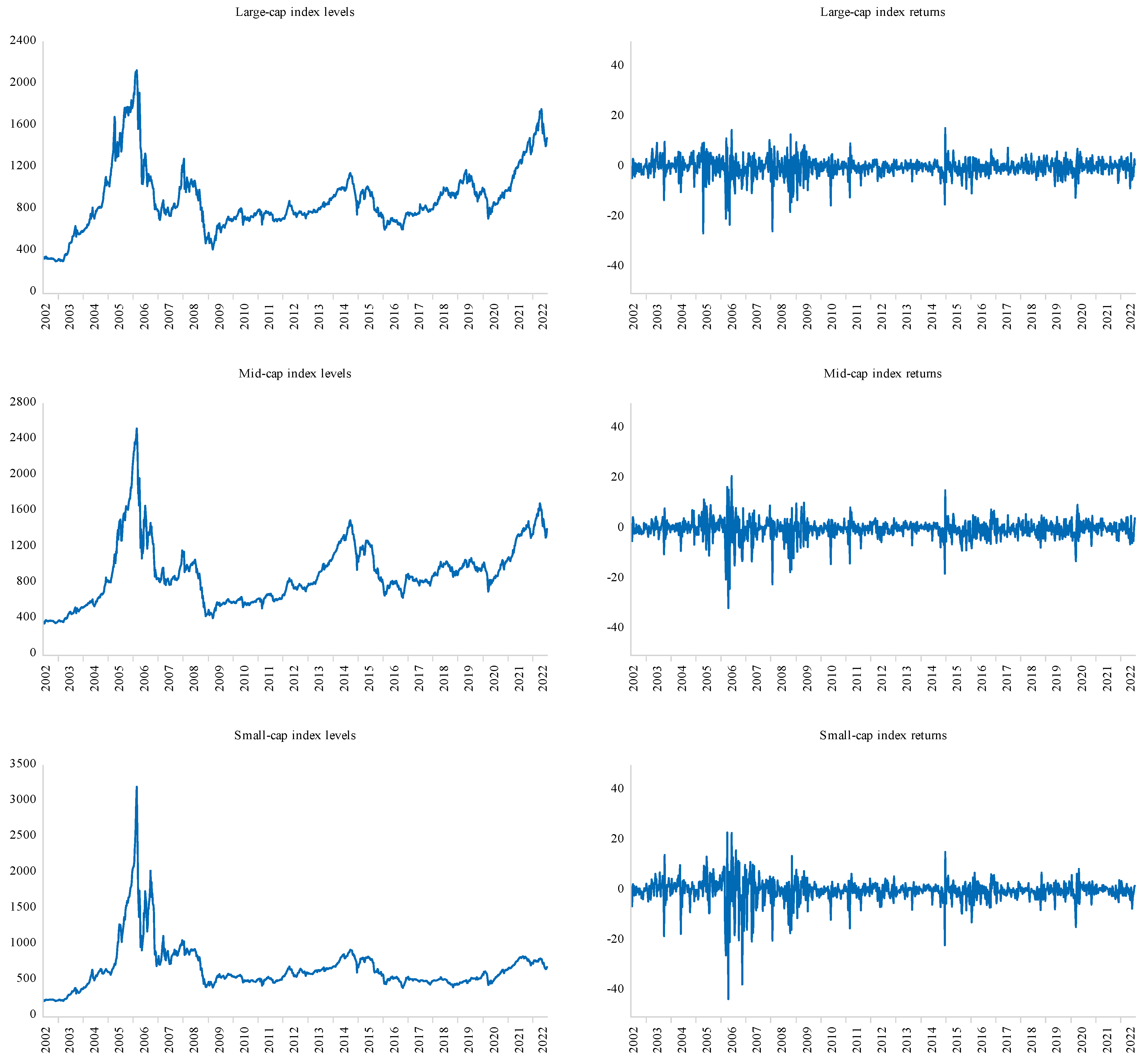
Figure 1. Time-series plots of weekly index levels and weekly returns of large-, mid-, and small-cap indices. Notes: The return series are expressed in percentages.
Ijfs 11 00113 g001
Figure 2. The annual return spread between large- and mid-cap (ML), large- and small-cap (LS), and mid- and small-cap (LS) indices. Source: computed by the author from the dataset of large-, mid-, and small-cap indices used in this study. Notes: The spread series are expressed in percentages.
Ijfs 11 00113 g002
Figure 3. Time-varying conditional correlations from the BEKK model with shift dummies.
Ijfs 11 00113 g003
Figure 4. Time-varying portfolio pairwise weights computed from the BEKK model with shift dummies.
Ijfs 11 00113 g004
Figure 5. Time-varying hedge ratios computed from the BEKK model with shift dummies.
Ijfs 11 00113 g005aIjfs 11 00113 g005b
Figure 6. Dynamic total volatility connectedness.
Ijfs 11 00113 g006
Figure 7. Dynamic net pairwise directional connectedness.
Ijfs 11 00113 g007
Table 1. Descriptive statistics.
LargeMidSmall
Mean0.140.130.10
Median0.400.410.47
Max15.7921.2923.39
Min−26.12−31.36−43.13
Std. Dev.3.853.904.71
Skewness−1.30−1.31−1.92
Kurtosis10.5612.8717.91
Student t1.171.060.72
Obs.105110511051
J-B2798.92 ***4562.39 ***10383.45 ***
ADF−32.03 ***−11.65 ***−15.54 ***
PP−32.06 ***−31.93 ***−29.37 ***
Q(4)3.3322.66 ***40.72 ***
ARCH–LM(4)108.43 ***233.38 ***135.15 ***
Notes: Student t = single-sample t test of the mean against a hypothesized value of zero; J–B = Jarque and Bera (1980) test for normality; ADF = augmented Dickey and Fuller (1981); PP = Phillips and Perron (1988); Q(4) = the Ljung–Box Q-statistics up to lag 4; ARCH (4) = the Engle (1982) Lagrange multiplier tests for autoregressive conditional heteroskedasticity in the residuals up to lag 4. *** denotes significance at the 1% level.
Table 2. The Engle–Ng sign bias test.
LargeMidSmall
Panel   A :   s t 2 = α 0 + α 1 d t 1 + α 2 d t 2 + α 3 d t 3 + e t
α 1 0.32 ** (2.41)0.19 (1.42)0.54 *** (5.43)
α 2 −0.10 (−0.73)−0.14 (−1.02)−0.09 (−0.54)
α 3 0.08 (0.61)−0.12 (−0.86)−0.03 (−0.18)
Joint test F 3 ,   1044 = 2.18 * F 3 ,   1044 = 1.26 F 3 ,   1044 = 3.61 **
Panel   B :   s t 2 = β 0 + β 1 d t 1 + β 2 d t 1 s t 1 + β 3 ( 1 d t 1 ) s t 1 + e t
β 1 0.19 (0.95)−0.11 (−0.56)0.57 ** (2.40)
β 2 −0.04 (−0.33)−0.03 (−0.25)0.13 (0.95)
β 3 −0.14 (−0.82)−0.44 ** (−2.34)−0.10 (−0.46)
Joint test F 3 ,   1046 = 2.12 * F 3 ,   1046 = 2.49 * F 3 ,   1046 = 3.86 ***
Notes: ***, **, and * denote significance at the 1%, 5% and 10% levels, respectively.
Table 3. Correlation matrix.
LargeMidSmall
Large1.00
Mid0.841.00
Small0.710.851.00
Table 4. Parameter estimates for the multivariate GARCH models.
BEKKBEKK with Shift Dummies
Coefft-Statp-ValueCoefft-Statp-Value
Mean
μ 1 0.294.570.000.304.720.00
ϕ 11 0.020.440.660.010.310.76
ϕ 12 0.040.840.400.051.040.30
ϕ 13 −0.03−1.080.28−0.04−1.170.24
μ 2 0.345.640.000.345.620.00
ϕ 21 0.041.070.290.041.100.27
ϕ 22 0.051.100.270.051.110.27
ϕ 23 −0.03−1.020.31−0.04−1.150.25
μ 3 0.274.490.000.284.480.00
ϕ 31 0.00−0.030.980.00−0.040.96
ϕ 32 0.122.860.000.122.600.01
ϕ 33 0.010.150.880.000.011.00
Variance
c 11 0.655.900.000.695.990.00
c 21 0.797.610.000.694.920.00
c 22 0.222.140.030.372.890.00
c 31 0.525.090.000.494.460.00
c 32 0.363.290.000.343.700.00
c 33 0.180.790.430.272.630.01
a 11 0.182.810.000.252.460.01
a 12 −0.03−0.650.52−0.01−0.070.94
a 13 −0.06−1.280.20−0.05−0.660.51
a 21 0.225.390.000.120.910.36
a 22 0.339.330.000.292.640.01
a 23 0.061.090.280.050.540.59
a 31 0.010.130.890.020.460.65
a 32 0.122.890.000.122.620.01
a 33 0.4510.480.000.458.540.00
b 11 0.9774.750.000.9424.200.00
b 12 0.012.960.000.010.110.92
b 13 0.032.610.010.040.930.35
b 21 −0.14−9.950.00−0.11−1.640.10
b 22 0.8440.150.000.8411.890.00
b 23 −0.11−4.220.00−0.11−1.720.09
b 31 0.032.730.010.020.670.50
b 32 −0.01−0.470.64−0.01−0.310.76
b 33 0.9251.130.000.9126.180.00
d 11 0.598.700.000.625.780.00
d 12 0.618.660.000.675.840.00
d 13 0.415.840.000.474.180.00
d 21 −0.23−4.060.00−0.37−1.610.11
d 22 −0.10−1.640.10−0.25−0.940.35
d 23 0.142.760.010.010.030.98
d 31 −0.32−5.390.00−0.27−2.360.02
d 32 −0.41−6.740.00−0.39−3.320.00
d 33 −0.41−4.960.00−0.41−3.690.00
Shape (t degrees)4.8312.880.004.9713.200.00
Log L−6601.23 −6591.54
AIC12.66 12.67
SC12.88 12.94
HQ12.66 12.67
Notes: Log L is the log likelihood, AIC is the Akaike information criterion, SC is the Schwarz information criterion, and HQ is the Hannan–Quinn information criterion.
Table 5. Diagnostic tests for the multivariate GARCH models.
BEKKBEKK with Shift Dummies
LargeMidSmallLargeMidSmall
Panel A:
Q 4   rstd 9.217.242.457.071.834.42
p-value0.060.120.650.130.770.35
Q 4   rstd 2 1.071.598.981.281.0031.14
p-value0.900.810.060.860.910.00
Panel B:
Nyblom’s test
Joint testTest Stat = 9.50p-value = 0.04Test Stat = 10.12p-value = 0.33
Notes: Q 4   rstd = Ljung–Box Q-statistics up to lag 4 applied to standardized residuals; Q 4   rstd 2 = Ljung–Box Q-statistics up to lag 4 applied to standardized residuals squared.
Table 6. Joint Wald test for the BEKK model.
The Portfolio of InterestMean EquationVariance Equation
All portfoliosThe null hypothesis of exogeneity
H 0 : ϕ i j = 0     i j ,
Test statistic: F 6 ,   = 2.17 **
Result: Reject H 0
The null hypothesis of diagonal BEKK
H 0 : a i j = b i j = 0     i j ,
Test statistic: F 12 ,   = 5.45 ***
Result: Reject H 0
LargeThe null hypothesis of exogeneity
H 0 :   ϕ 12 = ϕ 13 = 0
Test statistic: F 2 ,   = 0.53
Result: Accept H 0
The null hypothesis that shocks to the mid- and small portfolios do not affect the variance of interest:
  H 0 : a 21 = a 31 = b 21 = b 31 = 0
Test statistic: F 4 ,   = 6.03 ***
Result: Reject H 0
MidThe null hypothesis of exogeneity
H 0 :   ϕ 21 = ϕ 23 = 0 ,
Test statistic: F 2 ,   = 0.81
Result: Accept H 0
The null hypothesis that shocks to the large and small portfolios do not affect the variance of interest:
H 0 : a 12 = a 32 = b 12 = b 32 = 0
Test statistic: F 4 ,   = 2.38 **
Result: Reject H 0
SmallThe null hypothesis of exogeneity
H 0 :   ϕ 31 = ϕ 32 = 0 ,
Test statistic: F 2 ,   = 4.30 **
Result: Reject H 0
The null hypothesis that shocks to the large and mid-portfolios do not affect the variance of interest:
H 0 : a 13 = a 23 = b 13 = b 23 = 0
Test statistic: F 4 ,   = 2.30 *
Result: Reject H 0
All portfolios The null of symmetric behavior in variance
H 0 : d i j = 0     i   &   j ,
Test statistic: F 9 ,   = 10.12 ***
Result: Reject H 0
Notes: ***, **, and * denote significance at the 1%, 5% and 10% levels, respectively.
Table 7. Joint Wald test for the BEKK model with shift dummies.
The Portfolio of InterestMean EquationVariance Equation
All portfoliosThe null hypothesis of exogeneity
H 0 : ϕ i j = 0     i j ,
Test statistic: F 6 ,   = 1.97 *
Result: Reject H 0
The null hypothesis of diagonal BEKK
H 0 : a i j = b i j = 0     i j ,
Test statistic: F 12 ,   = 2.80 ***
Result: Reject H 0
LargeThe null hypothesis of exogeneity
H 0 :   ϕ 12 = ϕ 13 = 0
Test statistic: F 2 ,   = 0.80
Result: Accept H 0
The null hypothesis that shocks to the mid- and small portfolios do not affect the variance of interest:
H 0 : a 21 = a 31 = b 21 = b 31 = 0
Test statistic: F 4 ,   = 1.
Result: Accept H 0
MidThe null hypothesis of exogeneity
H 0 :   ϕ 21 = ϕ 23 = 0 ,
Test statistic: F 2 ,   = 1.05
Result: Accept H 0
The null hypothesis that shocks to the large and small portfolios do not affect the variance of interest:
H 0 : a 12 = a 32 = b 12 = b 32 = 0
Test statistic: F 4 ,   = 2.25 *
Result: Reject H 0
SmallThe null hypothesis of exogeneity
H 0 :   ϕ 31 = ϕ 32 = 0 ,
Test statistic: F 2 ,   = 4.37 **
Result: Reject H 0
The null hypothesis that shocks to the large and mid-portfolios do not affect the variance of interest:
H 0 : a 13 = a 23 = b 13 = b 23 = 0
Test statistic: F 4 ,   = 1.03
Result: Accept H 0
All portfolios The null of symmetric behavior in variance
H 0 : d i j = 0     i   &   j ,
Test statistic: F 9 ,   = 10.09 ***
Result: Reject H 0
Notes: ***, **, and * denote significance at the 1%, 5%, and 10% levels, respectively.
Table 8. Portfolio weights.
Mean Std. Dev. Min Max
Panel A: BEKK
L/M0.460.290.001.00
L/S0.510.330.001.00
M/S0.570.320.001.00
Panel B: BEKK with shift dummies
L/M0.460.290.001.00
L/S0.510.330.001.00
M/S0.580.330.001.00
Table 9. Hedge ratios.
Mean Std. Dev. Min Max
Panel A: BEKK
L/M0.790.160.371.23
L/S0.750.240.141.53
M/S0.850.210.361.62
Panel B: BEKK with shift dummies
L/M0.780.160.351.28
L/S0.740.240.131.50
M/S0.850.210.341.54
Table 10. Static volatility connectedness table.
From
ToLargeMidSmallContribution from Others
Large49.5227.5722.9150.48
Mid26.9246.9126.1753.09
Small21.9427.3950.6749.33
Contribution to others48.8654.9649.08152.89
Contribution including own98.37101.8799.75Total connectedness index
Net volatility connectedness −1.631.87−0.2550.96
Notes: The underlying variance decomposition is based upon a weekly VAR of order 2. The I ,   j - th value is the estimated contribution to the variance of 10-weeks-ahead weekly volatility forecast error of portfolio i coming from innovations to weekly volatility of portfolio j .
Disclaimer/Publisher’s Note: The statements, opinions and data contained in all publications are solely those of the individual author(s) and contributor(s) and not of MDPI and/or the editor(s). MDPI and/or the editor(s) disclaim responsibility for any injury to people or property resulting from any ideas, methods, instructions or products referred to in the content.