Abstract
In this paper we study the pricing of exchange options between two underlying assets whose dynamic show a stochastic correlation with random jumps. In particular, we consider a Ornstein-Uhlenbeck covariance model, with Levy Background Noise Processes driven by Inverse Gaussian subordinators. We use expansions in terms of Taylor polynomials and cubic splines to approximately compute the price of the derivative contract. Our findings show that the later approach provides an efficient way to compute the price when compared with a Monte Carlo method, while maintaining an equivalent degree of accuracy.
1. Introduction
In this paper we study the pricing of exchange options when the underlying assets have stochastic correlation with random jumps. More specifically, we consider an Ornstein-Uhlenbeck covariance process with Background Noise Levy Process (BNLP) driven by Inverse Gaussian subordinators. In order to calculate the price of the derivative contract we use expansions of the conditional price in terms of Taylor and cubic spline polynomials and compare the results with a computationally expensive Monte Carlo method.
Recently, the price of exchanges in models with stochastic volatilities and random jumps has been studied in several papers. Researches differ in the modeling of the correlation, volatilities and jumps, as well as in their numerical approaches. In Garces and Cheang (2021) for example the method of lines is successfully implemented. See also Alos and Rheinlander (2017); Kim and Park (2017); Pasricha and Goel (2022) for other techniques. Interesting applications in a context of credit risk can be found in Kim (2020); Pasricha and Goel (2019).
The exchange of two assets can be used to hedge against the changes in the price of underling assets by betting on the difference between both. The price of these instruments has been first considered in Margrabe (1978) under a bivariate Black-Scholes model, where a closed-form formula for the pricing is provided. Those results have been extended in Caldana and Fusai (2013); Caldana et al. (2015); Cheang and Chiarella (2011) to price the exchange in the case of a jump-diffusion model, while Bernard and Cui (2010) considers the pricing of the derivative contract under stochastic interest rates.
On the other hand, it is well known that constant correlation, constant volatilities and continuous trajectories are features no supported by empirical evidence. Some dynamic stochastic models for the covariance have been previously proposed, see for example Da Fonseca et al. (2008) for the popular Wishart model, Pigorsch and Stelzer (2007) for an Ornstein-Uhlenbeck Levy type model, Olivares et al. (2010) for a simple model based on a linear combination of Cox-Ingersol-Ross processes and finally an extension of Barndoff-Nielsen and Shephard (2001) to a multivariate setting proposed in Barndorff-Nielsen et al. (2002). Based on the later we study the integrated characteristic function, moments and pricing of the exchange.
Unfortunately, a closed-form pricing formula is not available when stochastic covariance and random jumps are considered. Approximations based on polynomial expansions of the price, after conditioning on the integrated covariance, allow for efficient and accurate calculations.
Starting with a pioneer idea in Hull and White (1987), Taylor expansions have been used to compute the price of spread options and other multivariate contracts. For example, a second order Taylor expansion has been successfully used in Li et al. (2008, 2010) to price spread options under a multivariate Black-Scholes model. As it is possible, based on the knowledge of the characteristic function, to compute mixed moments for the integrated covariance model an approach following the same idea seems feasible to be applied for the case studied in this paper. Moreover, other polynomial expansions such as cubic splines are also considered.
Our approach is in essence a combination of conditioning, polynomial expansions and a FFT inversion. Together with the existence of a closed-form expression for the price in the Black-Scholes setting it allows to value exchange options when considering stochastic correlation.
The organization of the paper is as follows. In Section 2 we introduce the main notations and discuss the pricing of the exchange option by polynomial expansions. In Section 3 we define the Ornstein-Uhlenbeck covariance process and compute the characteristic function of the integrated process and its moments. In Section 4 we discuss the implementation of the method, while numerical results allowing a comparison between the price obtained by Monte Carlo and polynomial approximations are shown in Section 5. Proofs of theoretical results are deferred to the appendix.
2. Pricing Exchange Options in Models with Stochastic Covariance
First, we introduce some notations. We denote by a matrix having ones in position and zeros otherwise. For a matrix A its trace is denoted by and its transpose by . For a vector V the expression denotes a diagonal matrix whose elements in the diagonal are the components of V. For two vectors x and y, represents its scalar product.
When l is an integer number, represents the l-th order derivative operator. To simplify notations we make .
Let be a filtered probability space. We denote by an equivalent martingale measure(EMM), and by r the (constant) interest rate or a vector with components equal to r. The filtration is assumed to verify the usual conditions, i.e., it is right-continuous and contains all events of probability zero.
The -algebra is defined for any as the -algebra generated by the random variables .
Also, we define the increments of the process as . For two squared integrable semi-martingales X and Y, defines their quadratic covariation process. The functions and represent respectively the characteristic function of the random variable X and the characteristic function of the random variable constrained to the interval , both under the chosen EMM.
A two-dimensional adapted stochastic process , where their components are prices of certain assets, is defined on the filtered probability space.
We describe the prices by:
where is the process of log-prices.
We assume that the process of log-prices has a dynamic under given by:
while is a matrix-valued stochastic process such that . Its components are denoted as , for .
Under , the process is a standard two-dimensional Brownian motion with independent components. The vector represents dividends on both assets. For any the conditional joint distribution of and its characteristic function are given in the elementary lemma below.
Lemma 1.
Let be a process driven by Equations (1) and (2) under an EMM . Then, conditionally on , the random variable follows a bivariate normal distribution. More precisely:
where has components
In particular, for a constant covariance process .
Moreover, the characteristic function of is:
where:
Proof.
From Equation (2) we have:
The third term in the equation above follows a bivariate normal distribution, conditionally on , with zero mean and elements of the covariance matrix given by:
Similarly:
On the other hand, from Equation (3) and the conditional normality of the log-prices:
□
The payoff of a European exchange option, with maturity at time is
where m is the number of assets of type two exchanged against c assets of type one.
A closed-form formula for the price of an exchange under a bivariate Black-Scholes model, i.e., the model given by Equation (2) with a constant covariance, starting at has been found in Margrabe (1978). This price, called Margrabe price, is denoted by .
On the other hand, the price of the exchange option under the full model, i.e., the one driven by equation Equation (2), after conditioning on is denoted by .
Notice that when conditioning on the covariance process the price process becomes a bivariate Gaussian model with deterministic and time-dependent volatilities and correlation.
Both prices are related by , as the price of the later is equivalent to the Margrabe price with constant covariance matrix .
Additionally, we denote by the unconditional price of the contract. To be more precise, the price of the exchange under the model (2) is given by:
where:
From the remark above and Lemma 1 a simple extension of Margrabe formula to the case of time-dependent deterministic covariance is given by:
with .
Remark 1.
The conditional Margrabe price depends on through the quantity . Consequently we write .
Pricing by Polynomial Expansions
In the general case of stochastic correlation there is not analogous to Margrabe pricing formula. It is possible to approximate the price of the exchange by a suitable expansion of in terms of Taylor polynomials around a point , typically around the mean value of the integrated process given by , or using a family of polynomials such cubic splines. We study in some details both approximations.
- (i)
- Taylor approximation.
The one-dimensional Taylor expansion of n-th order, denoted , around the value is given by:
A Taylor approximation of the price, taking into account Equation (4), is defined by:
Remark 2.
Notice that, in order to implement the approximation above we need the derivatives of the up to order n and the mixed moments of the components in the integrated covariance matrix .
Remark 3.
Sensitivities with respect to the parameters in the contract can be obtained in a similar way. For example, approximations of the deltas are:
- (ii)
- Approximation by cubic splines.
On an interval we consider a partition .
An approximation of based on cubic splines is thus given by:
The coefficients depend on the partition.
To smooth the curve additional conditions on the derivatives are usually imposed. Namely, , , where and are respectively the derivatives from the left and the right of the function at point .
Moreover, for end points in the interval we set . See Arcangeli et al. (2004) for a general account on splines and its implementation.
On the other hand, this approach requires the constrained moments of up to order n where the matrix M is:
To this end we first compute the corresponding characteristic function of the covariance process constrained to . Notice that:
The constrained moments of , assuming they exist, can be obtained by differentiating Equation (8) with respect to u and evaluating at .
3. An Ornstein-Uhlenbeck Stochastic Covariance Model
Our model is based on the general Ornstein-Uhlenbeck process with a Levy Background Noise Process (BDLP) as studied in Barndoff-Nielsen and Shephard (2001). It has been extended to a multidimensional setting in Barndorff-Nielsen et al. (2002).
We define a matrix-valued covariance process, based on independent Levy processes and , with respective characteristic exponents and .
The covariance process is defined for any by:
where is a deterministic orthonormal loading matrix.
The processes F and V correspond to idiosyncratic and common covariance factors respectively. Furthermore, we assume and are Ornstein-Ulenbeck Levy processes given by:
with BDLP denoted respectively by and , , for .
After applying Ito formula we have that the integrated processes corresponding to Equations (12) and (13) are:
To be more specific we consider Inverse Gaussian subordinators with respective characteristic exponents:
The integrated covariance process is then given by:
Its characteristic function is computed in the proposition below:
Theorem 1.
Let be the integrated covariance processes defined by Equation (18), with and following Ornstein-Ulenbeck processes having initial deterministic values and and independent Inverse Gaussian subordinators as BDLPs.
Denote by the characteristic functions, let be a matrix and . Then, for :
with:
and
Analogous expressions for and are obtained after replacing F by V.
Proof.
See Appendix A. □
Moments of the integrated process can be obtained from the derivatives of the integrated characteristic function evaluated at zero. To this end we need to compute the derivatives of expressions (19) and (20).
For simplicity we provisionally drop the dependence on V and F. Notice that is differentiable with respect to in a vicinity of zero. Moreover, at points different from zero:
For the case we take into account that to have:
The fact that the function is continuously differentiable on a vicinity of zero and continuous on the variable s on the interval allows to interchange derivative and integration by Lebesgue Dominated Convergence Theorem. Therefore, for :
At :
Moreover, for the n-th derivative is obtained as:
and evaluating at :
Proposition 1.
Let be the integrated covariance processes given by Equation (18), where and follow Ornstein-Ulenbeck processes with initial deterministic values and and independent Inverse Gaussian subordinators as BDLPs. Then, the first two moments of the elements in are given by:
where for :
Moreover, for :
for .
where for :
Proof of Proposition 1.
See Appendix A. □
The constrained moments of are needed in the cubic spline approaches. They are obtained via the constrained characteristic function in the proposition above.
Proposition 2.
Let be the integrated covariance processes defined by Equation (18), with and following Ornstein-Ulenbeck processes having initial deterministic values and and independent Inverse Gaussian subordinators as BDLPs.
Denote by the constrained characteristic function of . Then:
where and
Moreover, derivatives of the constrained characteristic function with respect to u evaluated at zero can be computed as:
for .
Here is the n-th derivative with respect to the variable u and is the j-th derivative of , also with respect to u and evaluated at .
Proof.
See Appendix A. □
4. Implementing Polynomial Expansions
In this section we precise the pricing formulas under the two approximations considered. Namely Taylor and splines approximation.
First, we implement the Taylor method based on Equation (6). To this end we first compute the Margrabe price under a model with time-dependent and deterministic volatilities and correlation, together with its derivatives evaluated at .
In order to simplify notations we introduce the following constants:
Then, by elementary calculations it follows that:
Hence, differentiating the Margrabe formula:
Therefore, the price based on the first order Taylor expansion can be computed as:
where .
For the second order expansion we compute:
Then, substituting Equation (31) into Equation (6):
In Figure 1 we show Margrabe price values as function of the variable v (blue curve) on the interval . For comparison, we also show Taylor polynomials of first (green line) and second (red line) order around the average log-price and benchmark parameters specified in Section 5. Both approximations are locally accurate but, for values farther from the differences are shown to be significant. It brings us the question of how often and how far departures from the average value occur.
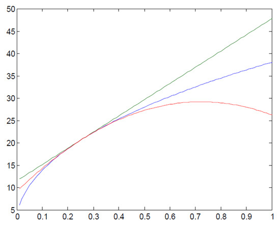
Figure 1.
Margrabe prices as function of the parameter v. Blue line represents the price. Green and red lines are respectively the first and second order Taylor approximations.
In Figure 2 the probability density function (p.d.f.) of the random variable obtained from simulated values of v is shown. It is estimated using a non-parametric Gaussian kernel. We observe that most values concentrate around the expansion point, whereas a low but significant frequency appear far from the mean, indicating the presence of a heavy-tailed probability distribution with positive skewness.
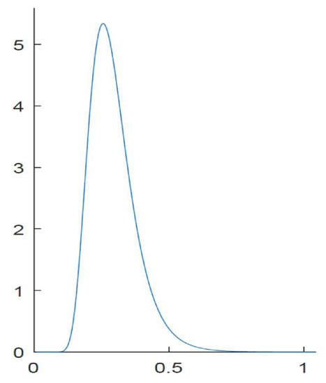
Figure 2.
Empirical probability density prices of obtained after simulations using Monte Carlo.
In order to overcome this potential inconvenient we consider a cubic splines approximation. The later adapts the expansion to the price behavior on different subintervals of .
To compute the constrained moments of we use Proposition 2, Equation (29). In order to simplify we assume initial values of the subordinators equal to zero. In Figure 3 a comparison between the Margrabe price is shown, while in Figure 4 the differences between Margrabe prices and its cubic spline approximation are shown. Despite some unstable behavior at the origin the fit is reasonable accurate.
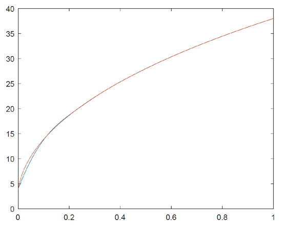
Figure 3.
Margrabe prices (blue line) and its cubic splines approximation (red line).
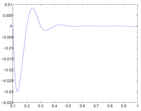
Figure 4.
Difference between Margrabe prices and its cubic spline approximation.
Therefore, we find that:
Higher moments are computed by recurrence:
Finally, centered moments are found from:
The calculations of the functions , , and their derivatives are shown in the Appendix A.
The constrained moments can be directly calculated from the p.d.f. of . In turn, the p.d.f. of is computed via its characteristic function by inverse FFT. To this end we define the grids:
where and are their respective lengths.
Hence, after applying the trapezoid rule:
with and and equal to one otherwise. The expression denotes the Fast fourier Transform of the sequence .
See Witkovsy (2016) for FFT applications in obtaining pdf’s and Hürlimann (2013) for a detailed analysis of different quadratures.
Notice that neither the joint characteristic function nor the p.d.f. of the pair of assets is known explicitly in the case of stochastic correlations. Hence, a direct application of a two dimensional FFT as in Hurd and Zhou (2010) or the approach in Caldana and Fusai (2013) to find the bounds of the price is not possible.
5. Numerical Results
We compare the polynomial methods and the Monte Carlo approach to pricing, for speed and accuracy. Our benchmark setting is given by a set of parameter values defining the model and the exchange contract. Contract parameters are selected within a reasonable range, according to usual practices, while the choosing of parameters in the model is made just with the purpose of illustrating the techniques. Notice that there are no benchmark values for the correlation as it depends on the specific assets considered. Nonetheless, the rationale in our choice is based on oil future prices per barrel for WTI and Brent types traded at NYSE. Initial prices are $ 100 and $ 96 respectively. Simulations show values within the range observed in the historic data of oil prices. On the other hand, this particular choice of parameters produces enough variability and jumps to impact the price of the derivative.
The calibration of the parameters, albeit a critical issue, is beyond the scope of the paper. See Pablo and Ciro (2023) for the use of a Generalized Method of Moments matching empirical and theoretical moments of both assets under a similar model.
The benchmark parameters for the model are and . For the contract we set and . The interest rate is .
We take the loading matrix A as an orthonormal rotation matrix with an angle , given by:
A direct Monte Carlo approach is costly as trajectories for both, the covariance process and the asset process, need to be simulated a large number of times. Alternatively, the iterative Formula (4) can be used to simplify calculations as, according to Lemma 1, conditionally on the covariance process the log-prices are normally distributed. It reduces the problem to calculate the discounted average of the price of an exchange contract under a deterministic time-dependent covariance, which still has a closed-form expression given in Equation (5). Hence, only the Ornstein-Ulenbeck covariance process needs to be simulated. We call this procedure a partial Monte Carlo approach.
Integrated Ornstein-Ulenbeck process values at time T, denoted by and are computed as discrete approximations of solutions of Equations (14) and (15) with a step , given respectively by:
where:
and ,
and , .
The symbol is the integer part of the real value x.
Next, the integrated covariance process is computed:
The price of the derivative contract is estimated from Equation (4) by the simulation of the covariance process and then computing the discounted average of the Margrabe prices evaluated at these simulated volatilities.
As an illustration, in Figure 5 three trajectories of an Inverse Gaussian process with parameters , are shown. Next, we generate the corresponding Ornstein-Uhlenbeck process as shown in Figure 6, starting at zero.
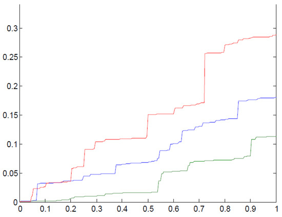
Figure 5.
Three realizations of the inverse Gamma process with parameters and .
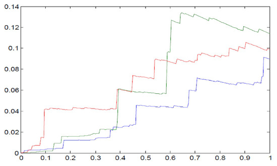
Figure 6.
Three realizations of the Ornstein-Uhlenbeck process.
Finally, in Figure 7, we show the trajectories of the correlation process obtained by dividing the covariance process by the product of volatilities from the underlying assets, with a load matrix defined by the angle . Both processes and are generated with the benchmark model parameters. Notice the correlation process exhibits jumps at random times, accounting for the effect of unexpected events.
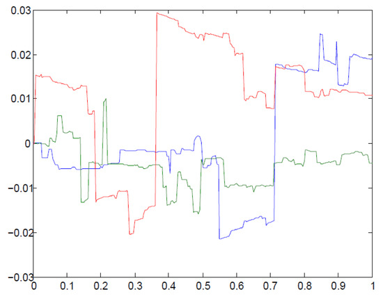
Figure 7.
Trajectories of the correlation process for the benchmark parameters.
In Table 1 different prices of the exchange contract for some notable values of the angle in the loading matrix are shown. In the case of the Monte Carlo approach we also calculate a 95% confidence interval for the price after 1 million simulations. We see that all methods, except the second order Taylor expansion, are within a similar range. First order Taylor price presents inaccuracies for other parameters of the subordinator processes, while the ones based on cubic splines and FFT developments are quite stable, their relative average error are approximately 0.018% when compared with the Monte Carlo price.

Table 1.
Prices obtained from different approximations and different values of using the benchmark parameters.
On the other hand, in Table 2 we can see the execution time (in sec.) for all five methods. The code has been written on a surface pro 4 i7 using MATLAB language. Cubic splines and FFT methods work, on average, respectively 16,488.8 and 18,408.4 times faster than Monte Carlo. The fact that FFT is slightly faster than cubic splines approximation comes at no surprise. It is well known that the former has a complexity compared with a of the later.
Table 2.
Average computer time (in seconds) for different pricing methods using the benchmark parameters and .
In implementing both approaches some quantities driving the numerical approximations are required. Namely, we need to decide on the truncation interval , in fixing a number of points in the grid for the Fourier transform and the number of points in the spline interpolation. The three factors require a compromise between accuracy and the amount of computation time. In the choice of the truncation interval we have tried to cover most of the support of the p.d.f. of the random variable (see Figure 4)which in turn depends on the parameters of both Inverse Gaussian subordinator processes. In our setting the interval was a reasonable trade-off. Of course, most of the time these parameters need to be estimated. In any case a significant probability mass is present in a neighborhood of zero, therefore seems a natural choice.
Regarding the number of points in the grid of the FFT calculation we have tested several powers of 2, ranging from to . There is not a significant change in the price across these values. We have set an intermediate value of . After this value the computation time explodes without a significant gain in accuracy. In order to implement the approach based on spline polynomials, we explored a range from to of interpolation points. After the price values are in close agreement with Monte Carlo and FFT. Numerical results improve if first derivatives at the end points of the expansion intervals are taken into account. They are available via Formula (30).
Notice that the FFT approach refers to the way the p.d.f. of the integrated stochastic volatility is obtained. It differs from the standard FFT pricing technique based on the Fourier transform of the payoff, see Carr and Madan (1999) for the latter. To calculate the unconditional expected value of the price an expansion based on Taylor or splines is still needed.
Alternatively, it may be possible to integrate directly Equation (4) once the p.d.f. of the integrated price is calculated. It leads to a double quadrature of a non-linear function, i.e., the Margrabe price, while avoiding the polynomial expansions. On the other hand, the expansions requires a single quadrature but at the expense of a lost in accuracy resulting from its inherent truncation.
Next, we analyze the sensitivities of the price of an exchange contract as function of the maturity and the difference between the parameters driving the volatilities of both assets.
Figure 8 shows the prices under a set of maturities ranging from 1 month to 5 years while keeping constant the remaining parameters in the benchmark set. Notice the damped oscillations of the price as the maturity increases, in contrast with the standard Margrabe exchange contract, showing the stabilizing effect of the integrated volatility for large values of T.
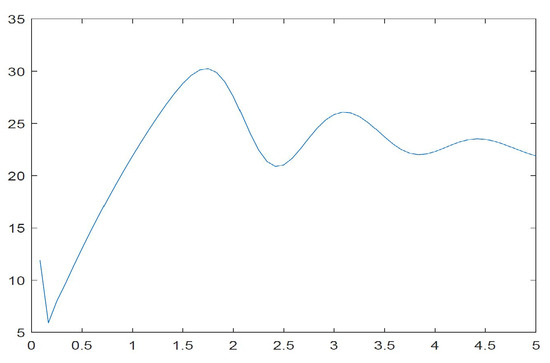
Figure 8.
Price of an exchange contract as function of maturity date.
In Figure 9 the curve shows the price in function of the parameter b in the inverse Gaussian distribution for the first asset, which drives down its volatility as it increases. As expected when the volatility decreases, i.e., the parameter b increases, anything else constant, the price of the exchange contract decreases.
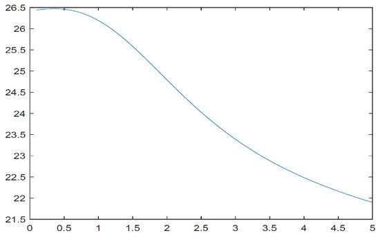
Figure 9.
Price of an exchange contract as function of the volatility.
6. Conclusions
We have discussed the pricing of exchange contracts under a dynamic model with a complex correlation structure capturing random jumps, heavy-tails, asymmetric and stochastic behavior. To this end we have proposed two approximate closed-form pricing methods based on cubic splines and Taylor approximations. To the extend of the investigation and the range of parameters considered, in the model, the contract and the numerical implementation, both approaches provide accurate and fast pricing estimates. Splines via FFT seems to have a slight edge over the direct application of cubic splines and Taylor expansion.
Author Contributions
Both authors (E.V. and P.O.) have worked on the conceptualization, methodology and formal analysis. Code has been written by P.O. All authors have read and agreed to the published version of the manuscript.
Funding
This research has been funded by the Institute of Environment at Florida International University, contribution # 1542.
Acknowledgments
This is contribution # 1542 from the Institute of Environment at Florida International University. The authors would like to thank the anonymous referees for their multiple suggestions that helped to improve the paper.
Conflicts of Interest
The authors declare no conflict of interest.
Appendix A
Proof of Theorem 1.
From Equations (14) and (15), and Levy-Khinchine formula we have, for :
where the last equality follows from the identity:
for a Levy process L with characteristic exponent and a continuous function f, see for example Cont and Tankov (2003). Similarly:
Next, the characteristic function for the integrated covariance process can be computed as:
On the other hand, from Equation (16) we have:
Then, for :
In what follows we use the identity:
where the complex-valued logarithmic function is defined according to the principal value of the argument.
Notice that:
Similarly:
whose solution is again .
An analysis at leads to the same conclusion.
Hence, for we have:
and
Then, substituting the expressions for arctan above into Equation (A1) we obtain Equation (19) after noticing that:
In a similar way we obtain Equation (20). Notice that in the case of , the equality is valid for all values of the matrix except when , which is equivalent to . □
Proof of Proposition 1.
The proof is straightforward. It is based on computing the first and second derivatives of the characteristic function evaluated at zero.
Hence, for the first moments we notice that:
Differentiating the characteristic function with respect to the components of the matrix and evaluating at we have:
From which, Equations (23) and (24) follow.
On the other hand the second partial derivatives after evaluating at zero are:
Therefore, we have:
In particular:
Also:
Finally:
□
Proof of Proposition 2.
Denote by the Fourier transform of .
Notice that:
and equal to if .
Hence:
Equation (27) easily follows from Theorem 1. The second part of the proposition follows from elementary differentiation. From which Equations (25)–(27) easily follow. □
Preliminary Calculations for the Constrained Moments
Some preliminary calculations of the constrained moments are given below.
Which leads to:
References
- Alos, Elisa, and Thorsten Rheinlander. 2017. Pricing and Hedging Margrabe Options with Stochastic Volatilities. Economic Working Papers 1475. Barcelona: Department of Economics and Business, Universitat Pompeu Fabra. [Google Scholar]
- Arcangeli, Remi, Maria Cruz Lopez de Silanes, and Juan Jose Torrens. 2004. Multidimensional Minimizing Splines: Theory and Applications. Berlin: Springer Sciences & Business Media. [Google Scholar]
- Barndoff-Nielsen, Ole E., and Neil J. Shephard. 2001. Non-gaussian Ornstein-Uhlenbeck-based models and some of their uses in financial economics. Journal of the Royal Statistical Society B 63: 142–9. [Google Scholar]
- Barndorff-Nielsen, Ole E., Elisa Nicolato, and Neil J. Shephard. 2002. Some recent problems in volatility stochastic models. Quantitative Financ 2: 11–23. [Google Scholar] [CrossRef]
- Bernard, Carole, and Zhenyu Cui. 2010. A note on exchange options under stochastic interest rates. Technical Report 6: 1–7. [Google Scholar] [CrossRef]
- Caldana, Ruggero, and Gianluca Fusai. 2013. A general closed-form spread option pricing formula. Journal of Banking & Finance 37: 4893–906. [Google Scholar] [CrossRef]
- Caldana, Ruggero, Gerald H.L. Cheang, Carl Chiarella, and Gianluca Fusai. 2015. Correction: Exchange option under jump-diffusion dynamics. Applied Mathematical Finance 22: 99–103. [Google Scholar] [CrossRef]
- Carr, Peter, and Dilip Madan. 1999. Option valuation using the fast fourier transform. Journal of Computational Finance 2: 61–73. [Google Scholar] [CrossRef]
- Cheang, Gerald H. L., and Carl Chiarella. 2011. Exchange options under jump-diffusion dynamics. Applied Mathematical Finance 18: 245–76. [Google Scholar] [CrossRef]
- Cont, Rama, and Peter Tankov. 2003. Financial Modelling with Jump Processes. Boca Raton: CRC Press. [Google Scholar]
- Da Fonseca, Jose, Martino Grasselli, and Claudio Tebaldi. 2008. Multifactor volatility heston model. Quantitative Finance 8: 591–604. [Google Scholar] [CrossRef]
- Garces, Len Patrick Dominic M., and Gerald H. L. Cheang. 2021. A numerical approach to pricing exchange options under stochastic volatility and jump-diffusion dynamics. Quantitative Finance 21: 2025–54. [Google Scholar] [CrossRef]
- Hurd, Thomas R., and Zhuowei Zhou. 2010. A Fourier transform method for spread option pricing. SIAM Journal of Financial Mathematics 1: 142–57. [Google Scholar] [CrossRef]
- Hürlimann, Werner. 2013. Improved fft approximations of probability functions based on modified quadrature rules. International Mathematical Forum 8: 829. [Google Scholar] [CrossRef]
- Hull, John C., and Alan White. 1987. The pricing of options on assets with stochastic volatilities. Journal of Finance 42: 281–300. [Google Scholar] [CrossRef]
- Kim, Jeong-Hoon, and Chang-Rae Park. 2017. A multiscale extension of the Margrabe formula under stochastic volatility. Chaos, Solitons and Fractals: Nonlinear Science, and Nonequilibrium and Complex Phenomena 97: 59–65. [Google Scholar] [CrossRef]
- Kim, Geonwoo. 2020. Valuation of Exchange Option with Credit Risk in a Hybrid Model. Mathematics 8: 2091. [Google Scholar] [CrossRef]
- Li, Minqiang, Shi-Jie Deng, and Jieyun Zhoc. 2008. Closed-form approximations for spread options prices and greeks. Journal of Derivatives 15: 58–80. [Google Scholar] [CrossRef]
- Li, Minqiang, Jieyun Zhou, and Shijie Deng. 2010. Multi-asset spread option pricing and hedging. Quantitative Finance 10: 305–24. [Google Scholar] [CrossRef]
- Margrabe, William. 1978. The value of an option to exchange one asset for another. The Journal of Finance 33: 177–86. [Google Scholar] [CrossRef]
- Olivares, Pablo, Marcos Escobar, Alexander Alvarez, and Luis Seco. 2010. Multivariate stochastic covariance models and applications to pricing and risk management. Journal of Financial Management and Decision Methods 6: 2. [Google Scholar]
- Pablo, Olivares, and Diaz Ciro. 2023. A finite elements approach for spread contract valuation via associated two-dimensional PIDE. Computational and Applied Mathematics 42: 15. [Google Scholar] [CrossRef]
- Pigorsch, Christian, and Robert Stelzer. A multivariate Ornstein-Uhlenbeck Type Stochastic Volatility Model. Available online: https://mediatum.ub.tum.de/1079183 (accessed on 14 December 2022).
- Pasricha, P., and A. Goel. 2019. Pricing vulnerable power exchange options in an intensity based framework. Journal of Computational and Applied Mathematics 355: 106–15. [Google Scholar] [CrossRef]
- Pasricha, P., and A. Goel. 2022. A closed-form pricing formula for European exchange options with stochastic volatility. Probability in the Engineering and Informational Sciences 36: 606–15. [Google Scholar] [CrossRef]
- Witkovsy, V. 2016. Numerical inversion of a characteristic function: An alternative tool to form the probability distribution of output quantity in linear measurement models. ACTA IMEKO 5: 32–44. [Google Scholar] [CrossRef]


Disclaimer/Publisher’s Note: The statements, opinions and data contained in all publications are solely those of the individual author(s) and contributor(s) and not of MDPI and/or the editor(s). MDPI and/or the editor(s) disclaim responsibility for any injury to people or property resulting from any ideas, methods, instructions or products referred to in the content. |
© 2023 by the authors. Licensee MDPI, Basel, Switzerland. This article is an open access article distributed under the terms and conditions of the Creative Commons Attribution (CC BY) license (https://creativecommons.org/licenses/by/4.0/).