Article

Uncertainty Shocks and Corporate Borrowing Constraints

1
College of Business, Texas A&M University-Corpus Christi, 6300 Ocean Drive, Corpus Christi, TX 78412, USA
2
Department of Economics and Statistics, California State University Los Angeles, 5154 State University Dr, Los Angeles, CA 90032, USA
*
Authors to whom correspondence should be addressed.
Int. J. Financial Stud. 2023, 11(1), 21; https://doi.org/10.3390/ijfs11010021
Submission received: 20 November 2022 / Revised: 30 December 2022 / Accepted: 10 January 2023 / Published: 19 January 2023
(This article belongs to the Special Issue Corporate Finance)

Abstract

:
In this paper, we study the effects of uncertainty shocks in a quantitative framework where firms in the corporate sector are constrained by credit. Specifically, we formulate borrowing constraints as a nested function that features both earnings and capital as alternative instruments for assessing credit worthiness, in line with recent trends in corporate finance. We find that the quantitative framework that incorporates only one instrument (capital or earnings) in the borrowing constraint falls short in matching the business cycle properties of the US economy in terms of the behavior of output, inflation, and the price markup which are an essential part of the literature on uncertainty shocks. Rather, a hybrid formulation of the borrowing constraint which accounts for both capital and earnings helps us bring the results in the quantitative model closer to the data.
JEL Classification:
E32; E510; E520

1. Introduction

This paper studies the interaction between financial frictions and uncertainty shocks, which are arguably two of the most important drivers of business cycle fluctuations (see, for instance, Bloom 2009; Jermann and Quadrini 2012). In particular, we explore the role of the credit channel of uncertainty shocks in driving macroeconomic conditions in the US economy. Through this channel, the rise in uncertainty about future productivity aggravates credit market conditions by increasing the information asymmetry between lenders and borrowers, thereby raising the cost of borrowing. The resultant decrease in the supply of credit leads to a fall in investment (see for example Aghion et al. 2010; Gilchrist et al. 2017; Bordo et al. 2016) 1. In the quantitative literature, uncertainty shocks are shown, in general, to exhibit properties of a negative demand shock (see for example Leduc and Liu 2016). Intuitively, the rise in uncertainty leads to an increase in precautionary behavior which puts a downward pressure on demand. To this extent, uncertainty shocks propagate in the economy through a countercyclical markup channel if prices are sufficiently sticky (see Born and Pfeifer 2014; Basu and Bundick 2017). The existence of the credit channel gives rise to supply side effects which would likely exacerbate the impact of the shock on the economy, or yet still alter the cyclical properties of the relevant variables.
In our set up, we model borrowing constraints as a nested function that features both corporate earnings and capital as alternative instruments for assessing credit worthiness in the corporate sector. This particular design allows us to analyze the macroeconomic effects of uncertainty shocks under alternative credit market settings: in one setting, borrowing is backed by the value of capital; in another setting, borrowing is tied exclusively to corporate earnings. Results under these two scenarios are compared to that of a baseline economy that does not feature any borrowing constraints. We also extend the analysis to look at a hybrid scenario where borrowing is tied to both corporate earnings and the value of capital stock. The inclusion of corporate earnings as an instrument in the constraint (in addition to capital) is motivated by recent trends in corporate finance which suggest a strong relationship between corporate earnings and firms’ access to credit. For example, Lian and Ma (2020), using micro-level data, find that about 80 percent of corporate loans are backed by cash flows, whereas the remaining 20 percent are backed by assets (capital).
In another study that examines 50,000 loan deals by 15,000 firms, Drechsel (2020) finds that about 35 percent of these deals are backed by cash flows as opposed to only 30 percent that are backed by corporate assets. Notwithstanding these findings, a majority of macroeconomic models that feature credit frictions tie borrowing to the value of corporate assets (see for example Kiyotaki and Moore 1997; Bernanke et al. 1999; Mendoza 2010). This marks a shift from earlier studies that primarily anchored borrowing to corporate cash flows (see Stiglitz and Weiss 1981; Holmstrom and Tirole 1997). Macroeconomic variables such as output, investment and employment are known to fluctuate significantly with credit market conditions. It would be interesting to see how differences in the assessment criteria for credit worthiness affects the behavior of the economy. Before we proceed, we note that, the phrases”capital-based” and ”asset-based” carry similar meaning in this paper. They are therefore used interchangeably henceforth.
In a preliminary analysis, we examine the effects of uncertainty shocks on the US economy using a Vector Auto-Regressive (VAR) model. In the model, we identify uncertainty shock using a Cholesky decomposition with the uncertainty proxy ordered first, as in Basu and Bundick (2017) and Leduc and Liu (2016). Using US data, we find that, while uncertainty shocks may display properties of a demand side shock (by generating lower prices concurrently with lower output), the price markup exhibits procyclical characteristics, as it declines (along side output) in response to the rise in uncertainty. This constitutes a disparity between the data and findings in the quantitative literature. The countercyclical markups obtained in quantitative models are contingent on the degree of price rigidity. In an environment where it is costly to adjust prices, firms respond to the decline in demand by moving downward along their marginal cost curves. This leads to an increase in the price markup concurrently with the lower output. In addition, given that prices are not fully rigid, the price level falls, however sluggishly, in response to the downward pressure on demand. Therefore, one possible explanation for procyclical markup in the data is that, in the US economy, prices are not rigid enough to generate countercyclical markups. Alternatively, it is likely that the presence of supply side effects keep the marginal cost sufficiently high to avoid a decline in the price markup. We explore variations in the formulation of the borrowing constraint in the DSGE model, expecting that the inherent supply side effects (through the credit channel) would help explain the disparity between the theory and the data.
In the VAR model, we also show that the credit spread rises in response to uncertainty shock, which is an indication of tightening in the credit market. Moreover, there is a decline in corporate earnings and the value of the capital stock which further aggravates the credit market by limiting the amount of collateral that is available to firms in the non-financial corporate sector to back-up borrowing. This leads to a fall in the flow of credit to the non-financial corporate sector. Consequently, investment, hours of work and output decline. In addition, the results show a very strong relationship between the collateral instruments (capital and earnings) on the one hand, and the flow of credit on the other hand. These findings imply that (on the account of the decline in both corporate earnings and the value of capital), both the earnings-based borrowing constraint and the asset-based borrowing constraint tighten while there is an elevation in uncertainty. This phenomenon highlights the significance of the credit channel for the propagation of uncertainty in the economy.
In the DSGE framework, we introduce uncertainty shocks as a second-moment perturbation which amplifies volatility in the total factor productivity (TFP). We then conduct a series of quantitative experiments to examine the macroeconomic effects of the shock under alternative formulations of the borrowing constraint. The results show that the formulation of the borrowing constraint is critical in determining how the uncertainty shock is characterized. In particular, we have the following findings: First, an increase in uncertainty about future productivity leads to tightening in both the earnings-based and the asset-based constraints, which is consistent with the results in the VAR model. Moreover, the constraint becomes tighter and remains so for a longer period of time if borrowing is constrained by asset as opposed to if it is constrained by earnings.
Secondly, the response of the price level to uncertainty shocks is also dependent on the formulation of the borrowing constraint. This is particularly important, as it indicates whether the shock can be characterized as a demand side shock or a supply side shock. While the price level falls in the model with capital-based constraint, it rises in the model with earnings-based constraint. To this end, the uncertainty shock displays properties of a demand side shock in the presence of the asset-based constraints. The opposite is true in the case of the model with earnings-based constraint. Third, following the rise in uncertainty, the price markup is countercyclical in the presence of the asset-based borrowing constraints. However, it becomes procyclical in the model with earnings-based borrowing constraint.
The last two findings show that the DSGE model with capital-based constraint matches the VAR model in terms of the behavior of output and the price level following uncertainty shocks: The shock exhibit properties of a demand side shock in both models. However, the DSGE model falls short in matching the cyclical properties of the price markup, as it generates countercyclical markups in contrast to that of the VAR model. On the other hand, the model with earnings-based constraint matches the VAR model in terms of the cyclical properties of the price markup, but falls short in terms of how the uncertainty shock is characterized: the shock is akin to a demand side shock in the VAR model, and a supply side shock in the DSGE model. Thus, including only earnings or capital as the only (collateral) instrument in the DSGE model, thus far, helps us explains part of the business cycle properties of the US economy, which leaves much to be desired.
In a special case with a hybrid formulation of the borrowing constraint where both capital and earnings are concurrently used as instruments for assessing credit worthiness, the results improve upon that of the other models where borrowing is constrained by only one of the instruments (assets or earnings), by matching the results in the VAR model. Specifically, both output and inflation decline in response to uncertainty shocks, which is an indication that the demand side effects dominate that of the supply side. At the same time, the price markup falls (concurrently with output) in response to the shock. To this end, the price markup is procyclical, with the correlation coefficient between the simulated output and the markup estimated to be about 0.50. This is also in line with the results in the VAR analysis (where the correlation is estimated to be about 0.12).
The above findings indicate that alternative formulations of credit constraints matter for the propagation of second-moment shocks in the DSGE model. The paper contributes to the plethora of literature on the effects of uncertainty shocks in a number of ways: First, it provides a unique formulation of credit constraints that is more in line with the current credit market. To the best of our knowledge, this is the first paper that explores alternative formulations of collateral constraints in a single study on uncertainty shocks. Secondly, the hybrid formulation of credit constraints in the DSGE model reverses the cyclical properties of the price mark-up (from countercyclical to procyclical) which puts it in alignment with the data, and constitutes an improvement on the existing models on uncertainty which largely yield countercyclical price mark-ups. This provides more insights into the understanding of uncertainty shocks and macroeconomic fluctuations.

1.1. A Brief Review of Borrowing Constraints and Access to Credit

There have been several micro-level studies on debt contracts (covenants) including those that look at alternative criteria for assessing credit worthiness (see for example Smith and Warner 1979; Malitz 1986; Begley 1994; Frank and Goyal 2009; De Fiore and Uhlig 2011; Bradley and Roberts 2015)2. Regardless of the differences in methods and objectives, the literature agrees on a variety of instruments by which credit worthiness is assessed. These include; Maximum Debt-to-Earnings before taxes (EBITDA), Maximum Interest Coverage (EBITDA/Interest), Maximum Fixed Charge Coverage (EBITDA/Coverage), Maximum Leverage Ratio, Maximum Capex, and Maximum Net Worth. Of the six instruments, three are related to earnings, with EBITDA being the primary indicator of this variable. Others such as the Maximum Leverage Ration is related to the firm’s assets. These covenants are legal requirements that a borrower (the firm) is obliged to satisfy throughout the lifetime of the loan. In Table 1, we present a few of the recently documented loan covenants that highlight the relative weight of each instrument in the loan contract.
Table 1 shows that corporate earnings constitutes the most significant part of the criteria for assessing credit worthiness. Notwithstanding, assets still remain an essential part of the criteria. These findings highlight the importance of incorporating both earnings and assets as instruments when studying the role of borrowing constraints in business cycle fluctuations in the economy. This paper moves in that direction.

1.2. Uncertainty Shocks in the Literature

Interests in the study of credit frictions and uncertainty have been evolving since Bernanke (1983) and Kiyotaki and Moore (1997). After a revived interest in the study of the macroeconomic effects of uncertainty shocks by Bloom (2009), several other works have explored different mechanisms through which uncertainty shock propagate in the economy (see for example Born and Pfeifer 2014; Carriero et al. 2015; Leduc and Liu 2016; Mumtaz and Surico 2018). Some of the mechanisms for the transmission of uncertainty shocks include the Oi–Hartman–Abel affects, real options effects, precautionary savings, and countercyclical markup channels.
The so-called Oi–Hartman–Abel effect (due to Oi 1961; Hartman 1972; Abel 1983) assumes that if profits are convex in demand or costs, then shocks to uncertainty about demand or cost increases expected benefits. Therefore, through the Oi–Hartman–Abel channel, uncertainty shocks are expansionary in nature. However, Born and Pfeifer (2014) and Basu and Bundick (2017) find that the presence of sticky prices opens the possibility for ’inverse-Oi–Hartman–Abel-effect’. In the sticky-price model, firms choose higher markups following an increase in uncertainty, thereby decreasing output. To this end, uncertainty shocks are contractionary through the countercyclical markup channel, even when profits are convex in demand or costs.
The real options channel of uncertainty is originally due to Bernanke (1983), The idea behind this mechanism is that firms are likely to wait for sometime in making decisions about new investments and hiring until there is a resolution of uncertainty shocks. In the case of the precautionary savings channel, uncertainty shocks increase consumers’ desire to save more, thereby decreasing consumers’ total expenditure (see Bansal and Yaron 2004). While a rise in precautionary savings might increase output in the long-run, the short-run effects are contractionary. Moreover, in the case of a highly open small economy, some of the savings will flow to foreign economies, which dampens both domestic demand and future growth (Fernandez-Villaverde et al. 2011).
Apart from the above named channels, there have been recent attempts to explore the credit channel for the propagation of uncertainty shocks in the economy (see Aghion et al. 2010; Gilchrist et al. 2017; Bordo et al. 2016; Valencia 2017; Cesa-Bianchi and Fernandez-Corugedo 2018; Choi et al. 2018; Brand et al. 2019). The goal is to see how the rise in uncertainty affects credit market conditions and how that transmits into the macroeconomy. The consensus is that, uncertainty shocks lead to a decline in the supply of credit in the economy, thereby decreasing investment.
In the formulation of credit frictions, most of the macroeconomic models in the literature rely on assets-based borrowing constraints. However, micro-level data show that creditors primarily use earnings (in one form or another) in the assessment of credit worthiness of firms (see Table 1). That is, earnings-based instruments are at least as important (if not more important) as asset-based instruments in the design of loan covenants. The choice of an instrument may play a significant role in determining the interaction between uncertainty shocks and credit constraints. In the DSGE model, we account for both earnings and assets as alternative instruments in the formulation of the borrowing constraint. Our analysis show that different specifications of the borrowing constraint lead to different conclusions regarding the transmission of uncertainty shocks, especially as it relates to the price markup channel.
The rest of the paper proceeds as follows. Section 2 presents the empirical analysis via a VAR model. Section 3 Presents the theoretical framework which builds on the standard New Keynesian model. Section 4 presents the numerical results where we discusses the implications of uncertainty shocks under alternative borrowing constraints. Finally, Section 5 concludes the paper.

2. Empirical Analysis

In this section, we present empirical analysis of the macroeconomic effects of uncertainty shocks using a Vector Auto Regressive (VAR) model. Specifically, we look at the response of macroeconomic variables such as output, consumption, and hours of work to uncertainty shocks in the US economy. We also evaluate the so-called credit channel of uncertainty by looking at the impact of these shocks on credit flow, the credit spread, corporate earnings and the value of capital stock. Moreover, cyclical properties of the price markup has been shown to be central to the propagation of uncertainty shocks in the economy. We therefore analyze the behavior of this variable in the light of these findings.

2.1. Empirical Specification: The VAR Model

In buiding the empirical framework, we employ a VAR model similar to the one discussed in Lutkepohl (2005). First, we present the model in the general form with n lags as:
w t = A W t 1 + B 0 y t + u t ,
where W t is the L × 1 vector of endogenous variables, A is an L × L n matrix of coefficients, B 0 is an L × M matrix of coefficients, and y t is the M × 1 vector of exogenous variables. In addition, u t is the L × 1 vector of white noise innovations, whereas W t is the L n × 1 matrix given by
W t = W t W t n + 1
Alternatively, the model can be written as:
W = B Z + U
where W = ( w 1 , . . . . . , w T ) , B = (A, B 0 ), Z = W 0 . . . . , W T 1 y 1 . . . . , y T , and U= ( u 1 ,.... u T ). W is L × T , B is L × ( L n + M ) , Z is ( L n + M ) × T , and U is L × T.

2.2. Variables in the System and Identification Strategy

There are eleven variables in the VAR model. In setting up the variables in the VAR model, We follow Drechsel (2020). The data for the analysis spans from the first quarter of 1986 to the last quarter of 2019. The ordering of the selected variables in the model is as follows:
( V A R 11 ) = Measure   of   uncertainty Relative   Price   of   Investment GDP   Deflator Hours   of   Work Capital   Stock   of   Non financial   Corporate   Sector Earnings   of   Non Financial   Corporate   Sector Credit   Flow   to   Non financial   Corporate   Sector Real   GDP Credit   Spread Federal   Funds   Rate Markup
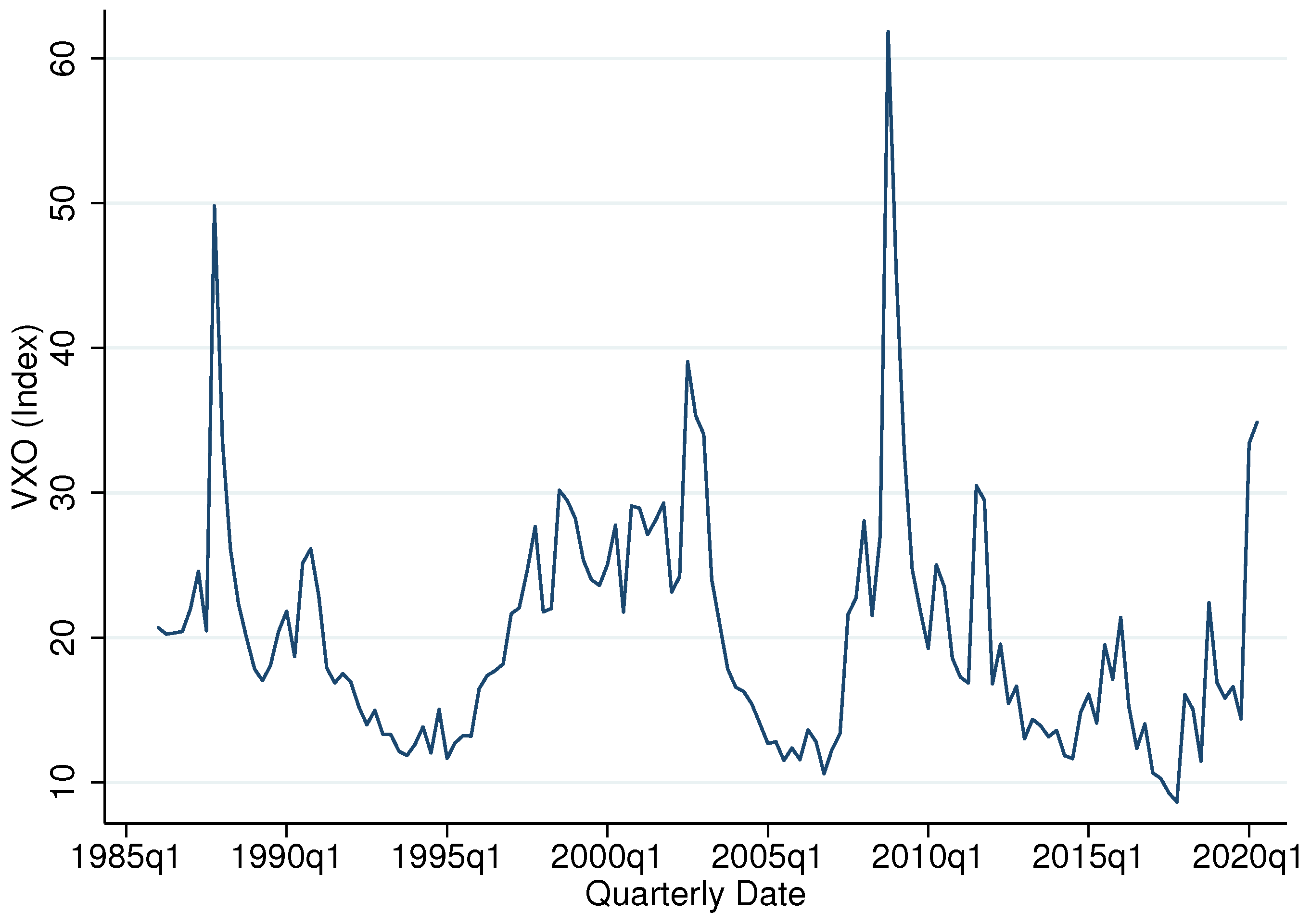
For a measure of uncertainty in the economy, we use the S&P 100 Volatility Index (VXO) as a proxy. Figure 1 shows the time-series of the VXO from the first quarter of 1986 to the first quarter of 2020. The cyclical property of the VXO makes it a very good fit for measuring uncertainty in the economy. As shown in the figure, the VXO is highly countercyclical. The data shows that the VXO rises significantly during economic downturns, with noticeable spikes during the crises of the 1990s, 2008/09, and the most recent and ongoing global health crisis precipitated by COVID-19. In addition to these features, data on the VXO are prevalent and is readily available in contrast to other competing indices.
Besides the VXO, we collect data on the relative price of investment, the price level, hours of work in the non-financial corporate sector, capital stock in non-financial corporate sector, corporate earnings, credit flow, GDP, the federal funds rate and the price markup. Except for the federal funds rate, all other variables in the model are in log levels. In addition, we identify uncertainty shock using a Cholesky identification scheme with the VXO ordered first. In the ordering of the variables we assume that an increase in uncertainty has an immediate impact on macroeconomic variables, while shocks unrelated to uncertainty do not affect volatility in the stock market. Our identification strategy is similar to the one followed by Leduc and Sill (2007), Auerbach and Gorodnichenko (2012), Leduc and Sill (2013), Leduc and Liu (2016), and Basu and Bundick (2017).
Sources of the data include the Federal Reserve Bank of St. Louis and the Bank of International Settlements (BIS). We deflate nominal variables with the consumption deflator. For data on corporate credit, we use credit to private non-financial sectors at market value. This is sourced from the Bank of International Settlements (BIS). In addition, given that the data are quarterly in nature, We select four lags of the model variables for the VAR estimation. Details on data construction and sources can be found in Appendix A.

2.3. The VAR Model Results

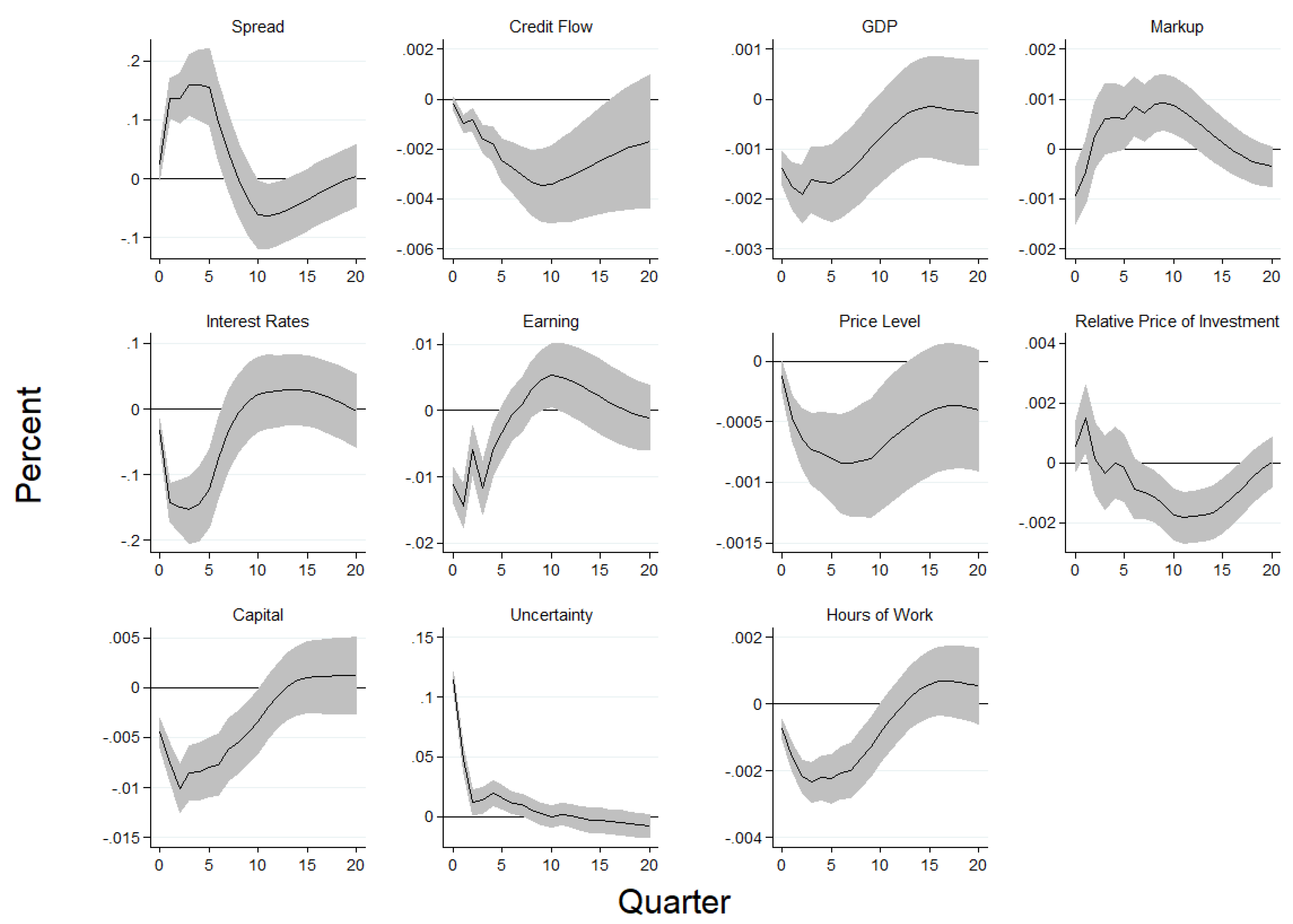
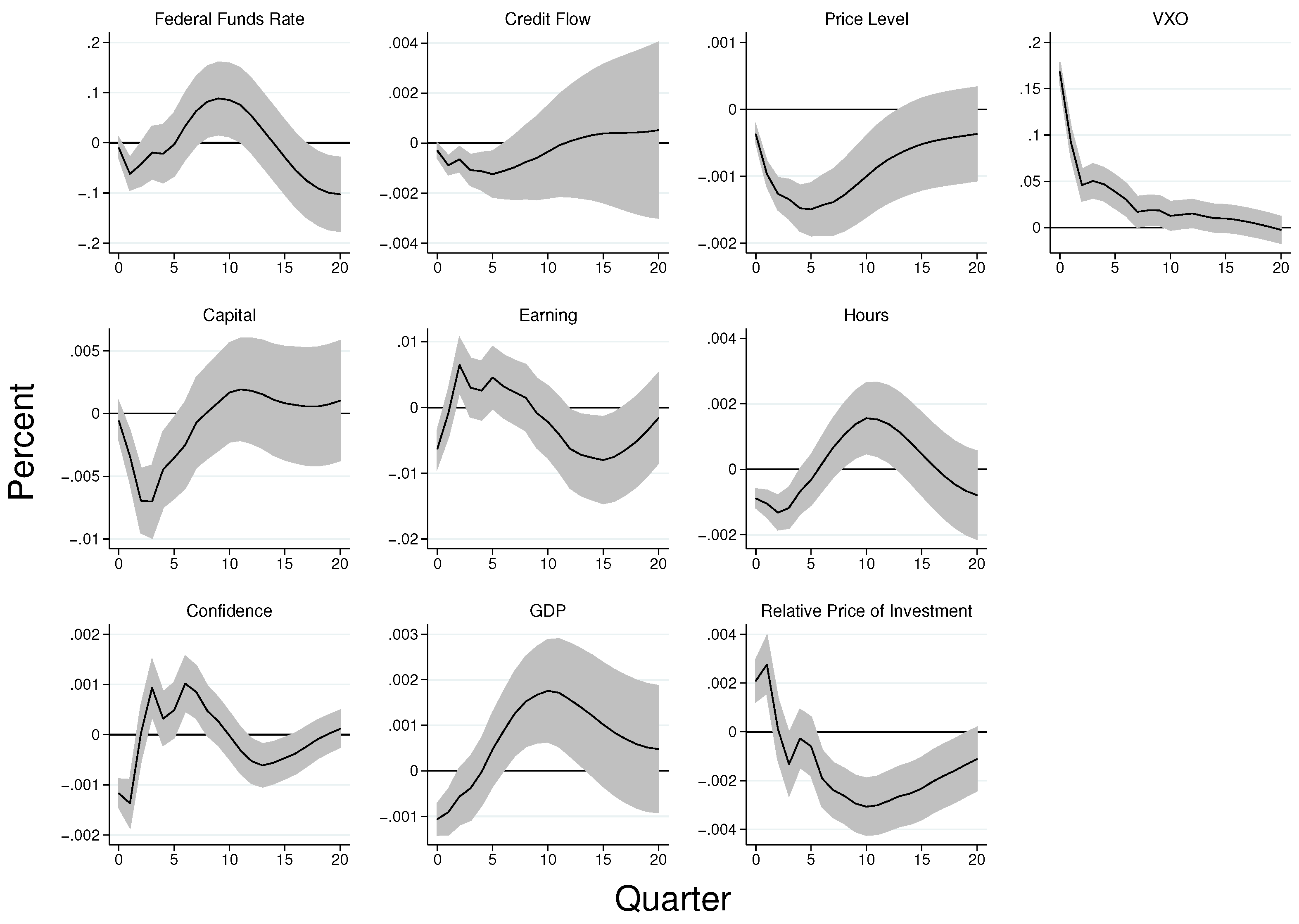
Figure 2 presents results of the VAR model. For each variable in the figure, the solid black line represents an average estimate of the impulse response whereas the shaded regions represent the range of the 68 percent confidence band interval (1% standard deviation shock). A one-standard deviation increase in uncertainty raises the VXO by 17.16% from the sample mean of 2.9346. The impact of the shock on the VXO indicates that the standard deviation of the uncertainty shock is about 5.8%. The figure also shows that the uncertainty shock leads to a decline in the hours of work. The decrease in hours of work remains significant for about six quarters, with the peak effect occurring after three quarters from the time of impact. The heightened uncertainty also leads to a persistent decline in the price level for consumer goods, which remains significant for about fifteen quarters from the time of innovation, with the peak occurring after five quarters.
In addition, the rise in uncertainty about the future increases the risk of default by firms in the non-financial corporate sector, which leads to a significant rise in the credit spread—an indication of tightening in the credit market. In addition, the shock gives rise to an increase in precautionary savings which leads to a fall in demand. The decline in demand puts a downward pressure on earnings and the stock of capital. Notably, earnings declines on impact but makes a quick and short-lived recovery after about three quarters. However, unlike earnings, the fall in the capital stock is gradual and lasts for about eight quarters, with a peak around the fourth quarter. In Table 1, we showed that both earnings and the capital stock constitute instruments by which firms in the non-financial corporate sector are assessed for credit worthiness. To this end, the decline in both earnings and the value of capital further constrains firms in the non-financial corporate sector by limiting the amount of collateral that is available to back-up borrowing. This leads to a decline in the flow of credit to firms in the non-financial corporate sector. As shown in the figure, the decline in credit flow is persistent and remains significant for about eight quarters, with the peak occurring around six quarters after the time of impact.
To demonstrate the strength of the association between these two instruments and the flow of credit to firms in the non-financial corporate sector, we look at the correlation between these variables in the simulated VAR model. We find the correlation coefficient between credit flow and the stock of capital to be about 0.90, whereas that of the credit flow and corporate earnings is about 0.96. These findings imply that (on the account of the decline in both corporate earnings and the value of capital), both the earnings-based constraints and the asset-based constraints tighten while there is a rise in uncertainty about the future. This phenomenon makes the effects of uncertainty on the credit market self-fulfilling, and highlights the significance of the credit channel for the propagation of uncertainty in the economy.
Furthermore, in the literature, uncertainty shocks are shown to exhibit properties of a negative demand shock (see for example Leduc and Liu 2016). It is therefore argued that uncertainty shocks propagate in the economy through a countercyclical markup channel if prices are sufficiently sticky (see Born and Pfeifer 2014; and Basu and Bundick 2017). To this end, the presence of sticky prices also implies that the price markup is procyclical following a negative supply shock (see Nekarda and Ramey 2021). The intuition is that, a rise in uncertainty causes an increase in precautionary savings which leads to a decline in demand. In an environment where it is costly to adjust prices, firms respond to the lower demand by moving downward along their marginal cost curves. This leads to an increase in the price markup (concurrently with the fall in output). In addition, given that prices are not fully rigid, the price level declines, however sluggishly, in response to the downward pressure on demand.
However, the results in the VAR model indicates that, while uncertainty shocks may display properties of a demand shock by generating lower output concurrently with lower prices, the proxy for the price markup exhibits procyclical characteristics, as it declines (with output) in response to the rise in uncertainty. Specifically, we find the correlation coefficient between the simulated output and the markup proxy to be about 0.12. One possible explanation for this outcome is that, in the US economy, prices are not rigid enough to cause firms to move downward along the marginal cost curve significantly enough to generate countercyclical price markup. That is, although both prices and the marginal cost may decline in response to the uncertainty shock, the decline in the price level is relatively larger, which leads to a fall in the price markup along with the decrease in output.

2.4. Robustness of the VAR Results

In this subsection, we carryout a similar analysis under an alternative measurements of uncertainty in order to provide a layer of robustness to the results in the VAR model. We do so by replacing VXO with the Economic Policy Uncertainty Index (EPUI) which is another popular proxy for uncertainty, developed by Baker et al. (2016). We also use an alternative measure of the price mark-up in the VAR model to see if that would impact the main conclusions in the benchmark model. In a separate analysis, we replace the federal Funds rate with the WU-Xia shadow rate which was developed by Wu and Xia (2016) to explain the macroeconomic effects of the unconventional monetary policy.

2.4.1. Using the EPUI Measure of Uncertainty

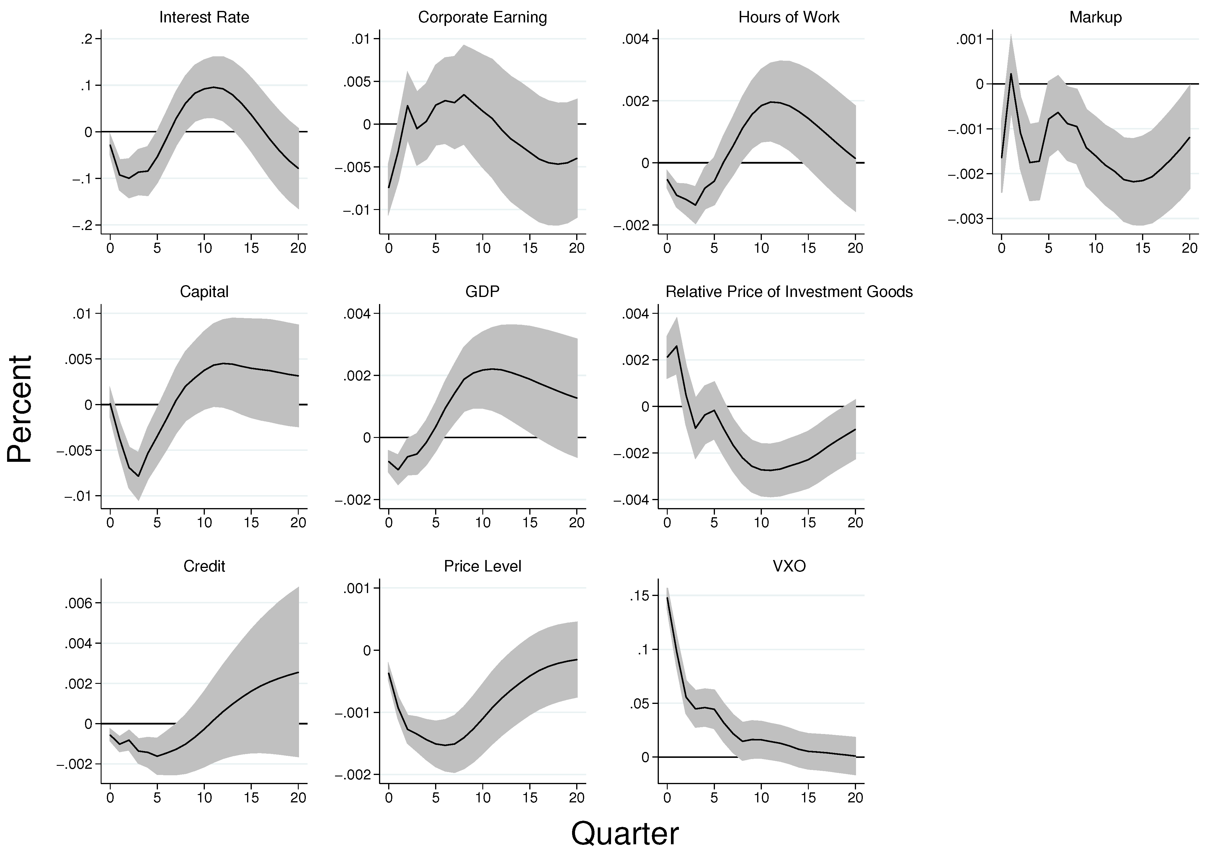
The negative effects of uncertainty shocks on the US economy, both at the firm level and in the macroeconomy, are not confined to the VXO measure of uncertainty. Similar qualitative results are achieved when the VXO is replaced with the economic policy uncertainty index (EPUI). The results are presented in Figure A3 (in the Appendix A). The results are consistent with that of the benchmark model. Following an increase in uncertainty, there is a decrease in hours of work for about ten quarters. Output and the price level also declines significantly for about 15 quarters following the innovation, which is an indication that the demand side effects of uncertainty dominates that of the supply side. However, the price mark-up declines (with output) in the first few quarters, which is contrary to findings in the quantitative literature that feature procyclical mark-ups. Moreover, the increase in uncertainty decreases firms’ earnings and capital stock, thereby hindering their access to external credit. Consequently, credit flow to the non-financial corporate sector declines and remains significantly low for more than 16 quarters of innovation.

2.4.2. Using Alternative Measurement of the Price Mark-Up

We now carryout a similar analysis under an alternative measurements of the price mark-up. Specifically, we use the time-series of markup developed by Nekarda and Ramey (2021) in the VAR model. Figure A4 presents the results. Again, in this setting, the main conclusions are upheld: That is, the demand side effects of uncertainty dominates the supply side effects, as both output and the price level decline in response to the rise in uncertainty. The price mar-up on the other hand exhibits procyclical properties. Furthermore, we show that these conclusions stand even if we change the ordering of the variables (see Figure A5).

2.4.3. Uncertainty Shocks under the WU-Xia Shadow Rate

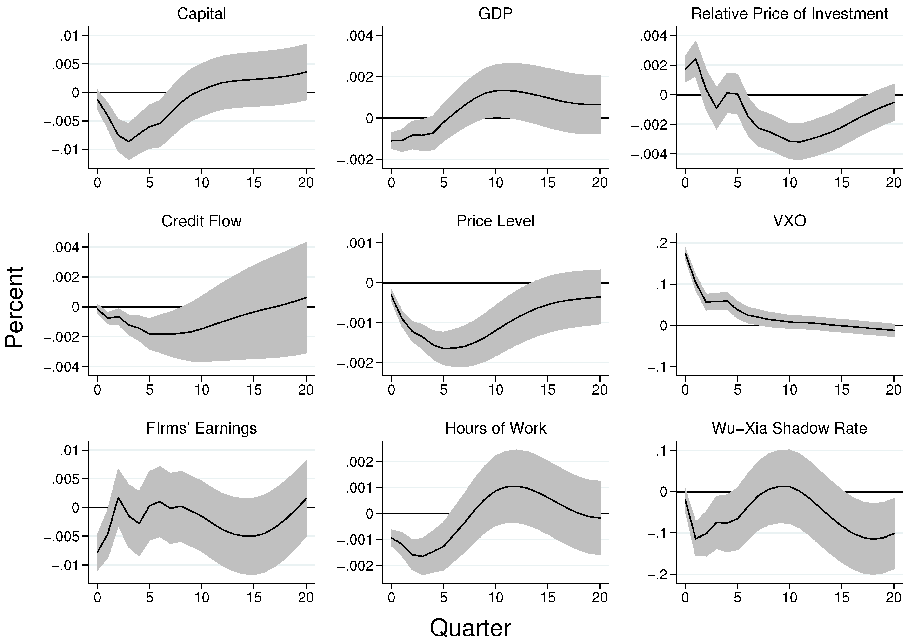
Wu and Xia (2016) developed an alternative measurement of the federal funds rate to explain the macroeconomic effects of unconventional monetary policy which is adopted by the Federal Reserve during periods of economic downturns. Using the Wu-Xia shadow rate as a stand-in for monetary policy would add to our understanding of the effects of uncertainty shocks under alternative monetary policy environments. Figure A6 presents the results. The results are consistent with that of the benchmark model. That is, uncertainty shocks lead to a decline in earnings and the capital stock. This hinders firms’ access to external credit which leads to lower output. ultimately affecting GDP negatively.

2.4.4. Is It about Uncertain Future or Bad Economic Times for Business?

The most important feature of the VXO is that it is countercyclical. Therefore, it is reasonable to interpret the results in the baseline model as an outcome that is driven by perceptions about the current (bad) economic times rather than adjustment towards an uncertain future. To resolve this, we construct a new VAR model with business sector confidence. The approach is similar to the one used by Baker et al. (2016) and Leduc and Liu (2016). The results are presented in Figure A7. The results show that the dynamic properties of the selected variables do not change relative to that of the baseline model even after we account for business confidence in the model. An increase in the VXO by one standard deviation decreases the price level and hours of work. In addition, there is an increase in the relative price of investment goods, which is likely an indication of the difficulties involved in adjusting investment. The value of capital stock owned by firms in the non-financial corporate decreases, as do their earnings, which makes it even more difficult for them to attract external credit. This events ultimately lead to a decline in GDP. The robustness of the results, even after accounting for business sector confidence suggest that perceptions about the current state of the economy is not the primary driver of the results as observed.

3. The Theoretical Model

The theoretical framework builds on the standard New Keynesian model.The model is composed of a continuum of infinitely lived households who derive utility from consumption and leisure. Moreover, the households supply labor to firms in the production sector. Firms in the production sector are monopolistically competitive. Each firm in this sector produces differentiated goods using a Cobb–Douglas production technology. Pricing in this sector is subject to a price adjustment cost as in Rotemberg (1982). In addition, firms in this sector face collateral requirements which limit their ability to borrow and finance new capital. Finally, there is a monetary authority which conducts monetary policy through a Taylor-type interest rate reaction function.

3.1. The Household Sector

There are j number of households with j ∈ [0,1]. In each period, a representative household supplies labor N j , t and derives utility from consumption C j , t , where C t = 0 1 [ ( C j , t ) ϵ 1 ϵ d j ] ϵ ϵ 1 . Total household expenditure on C j , t is then given by P j , t P t ϵ C t where P t = 0 1 [ ( P j , t ) ϵ 1 ϵ d j ] ϵ ϵ 1 is the price index. The household, given the intertemporal discount factor, maximizes utility which is governed by the following function:
E t t = 0 β t γ t l o g ( C j , t ) χ N j , t 1 + ν 1 + ν
where ν is the labor supply elasticity, and χ is the disutility of labor. In addition, γ t captures household preferences which evolves according to the following:
l o g γ t = ( 1 ρ γ ) l o g γ + ρ γ l o g γ t 1 + σ η t .
where ρ γ determines the persistence of demand shock and σ is the standard deviation of the shock. Each household maximizes equation 1 subject to the following budget constraint:
P j , t C j , t + B t + 1 W j , t N j , t + Π j , t + R t 1 B t T t
P j , t C j , t is nominal consumption expenditures, B t is the stock of savings with which a household enters a period, with R t 1 being the interest rate on that savings. In addition, Π j , t is a dividend distribution from the firm. Let us suppose that λ j , t is the multiplier on constraint Equation (3).
Solving the household’s problem and imposing symmetry among all households yields the following standard optimality conditions:
C j , t : λ j , t = γ t P j , t C j , t
B t + 1 : = λ t = β E t λ t + 1 R t π t 1 + 1
N j , t : γ t χ N j , t ν = λ t w t
Equation (4) is an expression for the marginal utility of consumption, Equations (5) is the consumption Euler which determines the optimal path for consumption, whereas Equation (6) is the labor supply condition.

3.2. Monopolistic Production Sector

Firms in this sector operate in a monopolistically competitive environment. Each firm i uses capital ( K i , t ) and labor ( N i , t ) as inputs to produce a differentiated final good ( Y i , t ), and faces a downward sloping demand for its products. The firm also faces a quadratic price adjustment cost as in Rotemberg (1982). Moreover, the firm faces collateral requirements which limit their ability to borrow and finance new capital. In addition, production in this sector is guided by the following Cobb–Douglas production technology.
Y i , t = A t K i , t α N i , t 1 α
A t is the total factor productivity (TFP) which evolves stochastically as follows:
l o g A t = ( 1 ρ A ) l o g A + ρ a l o g A t 1 + σ t A ε t A
where ρ A and σ t A capture the persistence and the time-varying volatility of total factor productivity, respectively. σ t A is assumed to follow an AR(1) process as follows:
σ t A = ( 1 ρ σ ) l o g σ A + ρ σ l o g σ t 1 A + σ σ t A ζ t ,
From (9), ζ t is the second-moment of the total factor productivity. We designate this variable as a measure of "uncertainty", as it amplifies the volatility in the total factor productivity. An increase in ζ t increases the uncertainty about future path of productivity in the economy. All the exogenous variables are independent and standard normal random variables.
Moreover, in line with the literature (see for example Drechsel 2020), we define the firm’s operational profit π t E as revenue net of overhead and labor costs. Alternatively, we refer to π t E as the firm’s earnings. This is determined as follows:
π i , t E = P i , t Y i , t P t W i , t P t N i , t .
In addition, capital, which is determined at the beginning of each period, evolves according to the following equation of motion:
K t + 1 = I t ϕ 2 I t K t δ 2 K t + ( 1 δ ) K t ,
where δ is the capital depreciation rate. In addition, the term ϕ 2 I t K t δ is a quadratic capital adjustment cost faced by the firm.

3.2.1. The Borrowing Constraint

As noted earlier, the firm, in order to invest in new capital issues a one-period debt D t + 1 which pays a gross return R t . For simplicity, we assume that the investment in new capital I t is equal to the debt issued:
I t = D t + 1
From the definition in (12), it follows that the payoff amount at the beginning of each period is R t 1 I t 1 .
Moreover, we assume that the firm is constrained in the credit market in that the debt that it issues must be backed by collateral. Specifically, we model the collateral constraint such that it nests both the value of capital stock and the firm’s current earnings as alternative collateral instruments. Specifically, the borrowing constraint is given as follows:
D t + 1 ρ θ π E π t E + ( 1 ρ ) θ k q t K t
where ρ is the probability that the new debt is backed by current earnings. Following the identity in Equation (12), we can rewrite Equation (13) as follows:
I t ρ θ π E π t E + ( 1 ρ ) θ k q t K t ,
In the analysis, we impose restrictions on Equation (14) in order to study the macroeconomic effects of uncertainty under alternative collateral requirements, including when investment is constrained by (a) the value capital only, and (b) current earnings only. Specifically, ρ assumes the following values:
p = 0 if   investment   is   constrained   by   capital   only . 1 if   investment   is   constrained   by   current   earnings   only .

3.2.2. Price Indexation

The firms in this sector are also assumed to index their prices, and are subject to a quadratic price adjustment cost a’ la Rotemberg (1982). Following Ireland (2007), we assume the price is indexed to both steady state inflation and past inflation. The price adjustment cost which is measured in units of the final good is therefore given as follows:
ψ 2 P i , t P i , t 1 π 1 I π t 1 I 1 2 P t Y t ,
where ψ is the price adjustment parameter which is constant. π is the steady state inflation, whereas π t 1 is the gross inflation rate between period t 2 and t 1 . In addition, I is the indexing parameter which takes values between 0 and 1. From this modified Rotemberg pricing model, we can see that price setting is either backward looking or forward looking depending on the value of I. If I is 0, it becomes cost-less to adjust prices to conform to steady state inflation. This gives rise to a completely forward looking Phillips curve. In contrast, if I is 1, it becomes cost-less to adjust prices in line with previous year’s inflation. In this case, the backward looking terms in the Phillips curve become as important as the forward looking terms.

3.2.3. The Firm’s Maximization Problem

The objective of the firm is to maximize the expected discounted dividends paid to its owners. Specifically, the firm’s expected profit function is given as:
Π i , t = E 0 [ t = 0 Λ t , t + 1 P i , t Y i , t p t W i , t N i , t R t 1 I i , t 1 ψ 2 P i , t P i , t 1 π 1 I π t 1 I 1 2 P t Y t
where Λ t , t + 1 is a stochastic discount factor defined as Λ t , t + 1 = β λ t + 1 γ t + t λ t γ t . The firm chooses n i , t , K t + 1 , I t , and P i , t to maximize Equation (15) subject to Equations (11) and (14), and its downward sloping demand function given by
Y i , t = p i , t p t ϵ Y t = A i , t K i , t α N i , t 1 α ,
The solution to the firm’s problem leads to the following optimality conditions:
W t = 1 α A t K α N t α m c t 1 + μ t p θ Π
μ t + β R t γ t + 1 γ t λ t + 1 λ t = q t 1 ϕ I t K t δ
q t = β γ t + 1 γ t λ t + 1 λ t { α A t + 1 K t + 1 α 1 N t + 1 1 α m c t + 1 + μ t + 1 1 p θ k + . . . q t + 1 1 δ + ϕ 2 I t + 1 K t + 1 δ 2 ϕ I t + 1 K t + 1 δ I t + 1 K t + 1 }
ε 1 = ε m c t ( ε 1 ) θ π t E p μ t ψ ( Υ t 1 ) Υ t β E t λ t + 1 λ t π t + 1 Y t + 1 Y t ( Υ t + 1 1 ) Υ t + 1
where
Υ t = π t π 1 I π t 1 I .

3.3. The Government

3.3.1. Fiscal Policy

In each period, the government finances its expenditure through lump-sum taxes T t , and by issuing bonds B t . The budget constraint of the government is given as:
R t π t 1 c B t 1 + T t = B t + P t G t ,
In addition, we assume g t , which is define as government spending relative to steady state output ( g t = G t Y ), evolves as follows:
l n g t = ( 1 ρ g ) g + ρ g g t 1 + ϵ g , t

3.3.2. Monetary Policy

Monetary policy in this economy is guided by the following Taylo type interest rate reaction function:
R t R = R t 1 R Ψ R Π t Π ( 1 Ψ R ) Ψ π Y t Y ( 1 Ψ R ) Ψ Y ω t R
where Ψ R in the interest rate smoothing parameter. That is, the Central Bank responds to deviations in output from its steady state levels ( Y ) , and deviations in inflation from a target value ( Π ). R is the steady-state interest rate which yields the target inflation in the long run. ω t R is an exogenous variable which follows an AR (1) process as follow:
l o g ω t R = ( 1 ρ ω ) ω R + ρ ω l o g ω t 1 R + σ R η t R ,
where ρ ω and σ R are the persistence and volatility of monetary policy shocks, respectively.

3.4. Market Clearing

In order to obtain the market clearing condition for the final goods market, we integrate the household budget constraint across all the entire household sector. Combined with the government budget constraint, we obtain the following:
P t C t + I t + P t G t = Π t + W t ( i ) N t ( i ) d i
Also from Equation (15), we have
Π t = Π t ( i ) d i = P t ( i ) Y t ( i ) d i W t N t R t 1 I t ϕ 2 P i , t P i , t 1 π 1 I π t 1 I 1 2 Y i , t ] ,
Now, we can combine Equations (25) and (26) to obtain the following:
P t C t + P t I t + P t G t = P t Y t ψ 2 ( Υ t 1 ) 2 P t Y t
For simplicity, we set G t equal to 0, implying that:
Y t = C t + I t + ψ 2 ( Υ t 1 ) 2 Y t .

4. Numerical Results

4.1. Calibration

Several structural parameters are calibrated to match the steady state values of the model. For those parameters that do not affect the model’s steady state, we set values that are consistent with the literature. The structural parameters to calibrate include β , the household discount factor; ψ , the price adjustment cost parameter; π , inflation target; Ψ π , the Taylor rule coefficient for inflation; Ψ y , the Taylor rule coefficient for output; ϕ , the capital adjustment cost parameter; χ , the disutility of labor; ρ , probability of investment being backed by earnings; α , the output elasticity of capital; ν , the elasticity of labor supply. In addition to the structural parameters, the parameters of the shock processes are also calibrated. Table 2 below summarizes the calibrated values of model parameters.
The household discount factor β is set to be 0.99, which represents the steady-state value of interest rate to be 4 percent per year. The steady-state inflation ( π ) is set to 1.0045 in accordance with Leduc and Liu (2016), which represents the Federal Reserve’s inflation objective. Frisch elasticity of labor supply ν is fixed at 1 so that the steady state value of labor (N) is calculated to be 0.33. Similarly, we set the value of disutility of labor supply χ to be 0.564 to match the steady state value of labor supply. Values of parameters related to nominal rigidities are calibrated according to the literature. In accordance with Faia (2008), we set the value of markup of prices over marginal cost to 0.2. That is, the value of the price elasticity of demand ( ϵ ) is fixed to 6. We calibrate the value of price stickiness parameter ( ψ ) = 110, which implies that prices are reset once every four quarters. The value of investment adjustment cost ϕ is calibrated to be 2.09, which is in line with the previous estimate from Basu and Bundick (2017). The Taylor rule parameters are set to Ψ π = 2.03, Ψ y = 0.3 , and Ψ R = 0.9, which are in line with the estimates from Smets and Wouters (2007). We follow Smets and Wouters (2007) in calibrating the parameters in the first order technology shock. For instance, the average standard deviation is set to be 0.01 and and the persistence parameter is fixed at 0.95.
The parameters in the collateral constraint (Equation (13)) are either calibrated in accordance with the literature or matched to the data. The value of θ k is set to 0.067, which is the average ratio of credit to capital, obtained from the empirical analysis. The fraction of corporate earnings that may be pledged, θ π t E is fixed to 5.77, which, again represents the average ratio of credit to earnings. We calibrate those values from the VAR model. For ρ , which is the probability of investment being backed by earnings, we set this value equal to 1 if borrowing is backed exclusively by earnings, and 0 if borrowing is backed exclusively by capital. For a hybrid formulation of the borrowing constraints which accounts for both assets and earnings as collateral instruments (as in our special case), we set this parameter equal to 0.8 in conformity with the data (see Table 1).
With regards to the uncertainty shock, we set the persistence and standard deviation in accordance with the baseline VAR model. The VAR results suggests that a standard deviation increase in uncertainty increases the VXO by 0.1716 units compared to the sample mean of 2.9346. Therefore, the uncertainty shock is equivalent to 5.8% of the increases in the uncertainty variable relative to mean. Since the standard deviation is 1% in the model, the standard deviation of uncertainty is set to be equal to 0.058.
The VAR model results also suggests that in one year, consumers’ perceived uncertainty decreases to about 30% of its peak. Since we assume the uncertainty process is governed by an AR (1) process, uncertainty persistence ρ γ manifests as 0.4 in our quarterly model, i.e., 0.74≈ 0.4.

4.2. The Macroeconomic Effects of Uncertainty Shock

This subsection discusses the results of the DSGE model. We obtain the effects of uncertainty shocks in the model by implementing a third-order perturbation in Dynare software as in Adjemian et al. (2011). In the process, Dynare calculates the model’s rational expectations solutions using the k-order Taylor series approximation around the steady-state model, which is presented in Appendix B.1. Before we proceed, we note that, the phrases “capital-based” and “asset-based” carry the same meaning in this paper. They are therefore used interchangeably.

4.2.1. Borrowing Constraints and the Price Markup

The price markup plays a very important role in driving the results in this paper, owing to the relationship between the markup and earnings. Therefore, before we analyse the model numerically, we first explore the interaction between the borrowing constraint and the price markup analytically. First, recall the nested borrowing constraint (Equation (13)). Suppose, we set ρ = 1 assuming that only the earnings-based constraint is binding, we obtain the following:
D t + 1 θ π t E π t E
where the real earnings π t E of a representative firm is given as follows:
π t E = Y t W t N t
The firms’ price markup is defined as the ratio of the price to marginal costs
ϰ t = P t M C t = 1 m c t .
Using the Cobb–Douglas production function (7) and Equation (17), we can rewrite Equation (30) as:
π t E = A t K t α N t 1 α 1 ( 1 α ) W t ( 1 α ) A t K t α N t α
which, combined with Equation (31) yields
π t E = Y t 1 ( 1 α ) ϰ t 1 1 + θ π
Equation (33) shows that real earnings is positively related to both output and the price markup. It is also clear from (31) that, for a given price level, increasing the price markup will require the firm to move downward along the marginal cost curve, and by doing so, cuts output, which negatively impacts real earnings. The degree of price rigidity therefore plays a significant role in determining the dynamic properties of the price markup. Moreover, if we combine (29) and (33), we obtain the borrowing constraint in terms of output and the markup as follows:
D t + 1 θ π t E Y t 1 ( 1 α ) ϰ t 1 1 + θ π .
From (34), we can see the interaction between the borrowing constraint, the price markup and output. The behavior of these two variables (output and markup) therefore have implications for tightness in the credit market and for the flow of credit to firms in the non-financial corporate sector. In the benchmark VAR analysis, credit to the non-financial corporate sector is highly procyclical, with the correlation coefficient between output and credit flow being 0.99. Similarly, earnings from this sector is also highly procyclical. The correlation coefficient between output and earning is found to be 0.97. These findings are in line with Equations (33) and (34). Moreover, such an explicit relationship between the markup and financial friction is not present in the capital-based borrowing constraints.

4.2.2. Earnings-Based Constraints vs. Asset-Based Constraints

Figure 3 presents the impulse responses of selected variables to uncertainty shock. Results are presented for 3 alternative models: a model that features capital-based borrowing constraints, one with earnings-based borrowing constraints and a baseline model without any credit frictions. A few comments are in order. Generally, the increase in uncertainty about future productivity negatively impacts the economy regardless of whether credit frictions are present or not. In particular, output, consumption, hours of work and real wages decline on impact under all three models, which is expected. However, the behavior of the price level differs in terms of the direction. This is particularly important, as it indicates whether the uncertainty shock can be characterized as a demand side shock or a supply side shock. While the price level falls in the baseline model and the model with capital-based constraint, it rises in the model with earnings-based constraints. To this end, the uncertainty shock displays properties of a supply side shock in the presence of the earnings-based borrowing constraints. The opposite is true in the case of the model with capital-based borrowing constraints and the baseline frictionless model. The mechanism driving this outcome is elaborated in what follows (when we discussed the properties of the price markup).
Moreover, there is tightening in both the earnings-based constraint and the capital-based constraints in response to the uncertain economic environment, which is evident in the behavior of the (Lagrange) multiplier. This outcome is consistent with the analysis in the VAR model. The rise in uncertainty leads to an increase in precautionary savings. The resultant decline in demand makes the corporate sector potentially less profitable. The increasing prospects of loan defaults by firms in the non-financial corporate sector elevates the risks associated with lending. This makes the borrowing constraint tighter. Moreover, the ensuing decline in the value of capital and earnings (the two instruments that constrain borrowing) makes it even harder for firms to access credit which induces further tightening in the credit market. In addition, in terms of the magnitude, the results indicate that the borrowing constraint becomes relatively less tight and remains so for a longer period if borrowing is constrained by earnings compared to that of the model where borrowing is constrained by capital. The relatively less tightening of the earnings-based constraints leads to a rise in the flow of credit to the non-financial corporate sector. To explain the disparities between the two credit constrained models in terms of the tightness in the credit market and the response of the price level, we turn to the behavior of the price markup, which we discuss next.
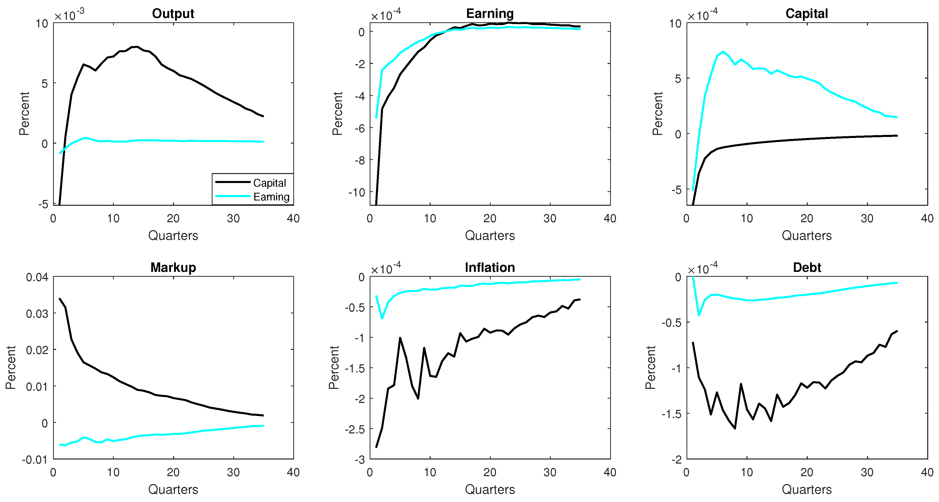
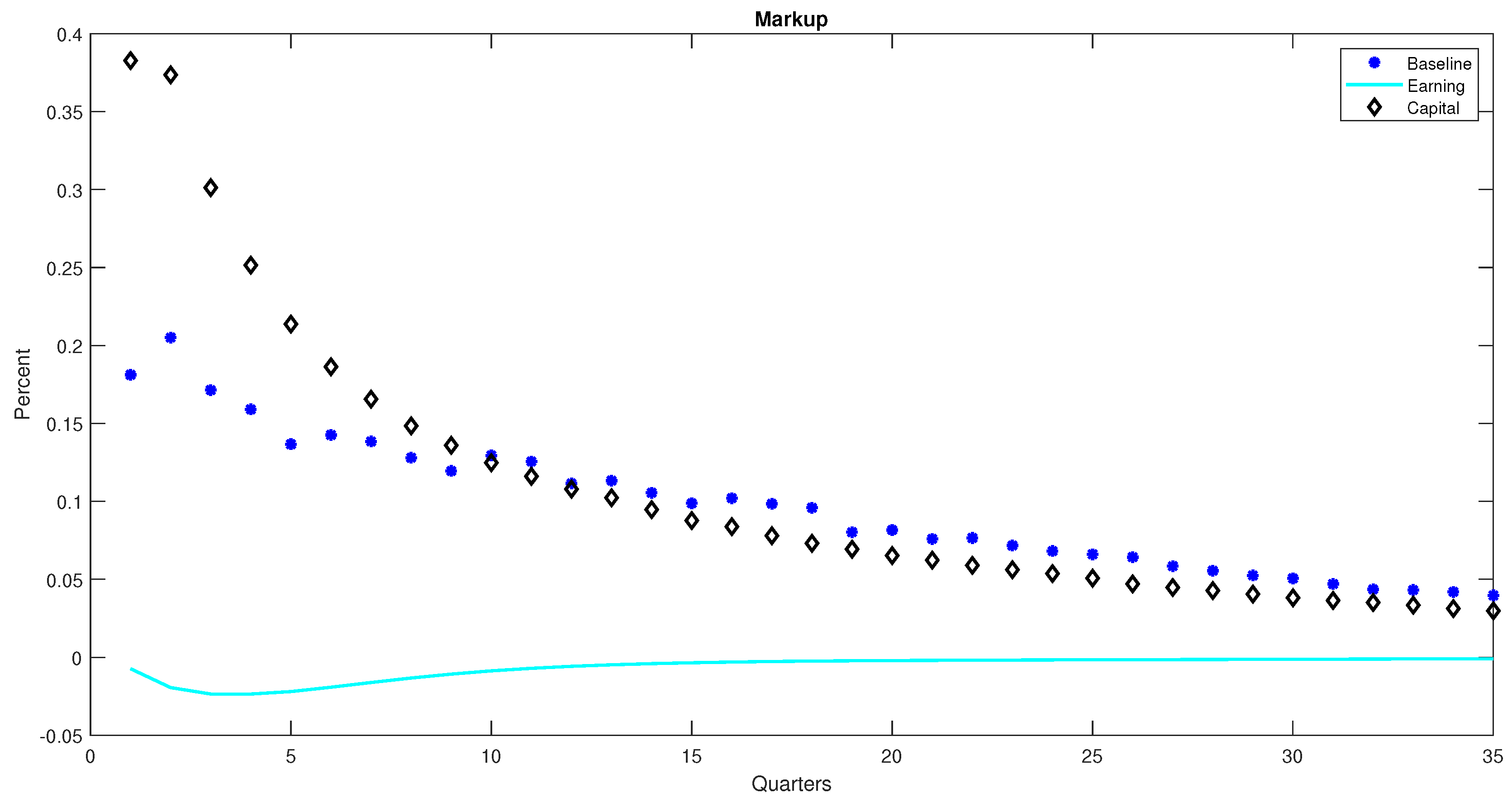
The cyclical properties of the price markup is an essential part of our results. Figure 4 reports the impulse responses of the price markup to uncertainty shock. As shown, the markup exhibits procyclical characteristics in the presence of the earnings-based borrowing constraints. However, it becomes countercyclical in both the frictionless model and the model with asset-based borrowing constraint. In the literature, uncertainty shocks are shown to exhibit properties of a negative demand shock (see Leduc and Liu (2016)). To this extent, uncertainty shocks propagate in the economy through a countercyclical markup channel if prices are sufficiently sticky (see for example Born and Pfeifer (2014); and Basu and Bundick (2017)). The presence of sticky prices also implies that the price markup is procyclical following a negative supply shock (see Nekarda and Ramey 2021). In the standard model without credit constraints, a rise in uncertainty leads to a decline in demand. In addition, in an environment where it is costly to adjust prices, firms respond to the decline in demand by moving downward along their marginal cost curves. This leads to an increase in the price markup (see Figure 4) concurrently with the fall in output. In addition, given that prices are not fully rigid, the price level falls, however sluggishly, in response to the downward pressure on demand.
In the presence of the capital-based borrowing constraint, the elevated risk of defaults in the credit market leads to an increase in the cost of borrowing. Moreover, the decline in the value of assets renders the borrowing constraint even tighter, thereby limiting the flow of credit to firms in the non-financial corporate sector. This leads to a shift in the firm’s marginal cost curve. Since prices are sticky, the firm has the incentive to move significantly downward along the new marginal cost curve, thereby lowering output beyond that of the baseline frictionless economy (see Figure 2). As a result, the price markup rises more compared to that of the baseline model. In addition, the decline in the price level indicate that the demand side effects dominate the supply side effects. Therefore, like that of the baseline model, the cyclical properties of the price level and the markup align with findings in the literature (see Leduc and Liu 2016; Born and Pfeifer 2014; and Basu and Bundick 2017).
In the model with earnings-based constraint, both output and the price markup decline on impact following the rise in uncertainty. However, the decline in output is short-lived, whereas that of the price markup persists for a longer period of time. Consequently, the price markup is weakly procyclical, with the correlation coefficient between the price markup and output reported to be about 0.024. At the same time the price level rises in response to the shock. By the behavior of the price markup and the price level, uncertainty shocks exhibit properties of a supply side shock in the presence of the earnings-based borrowing constraints. Put differently, the supply side effects of uncertainty dominate that of the demand side if borrowing is constrained by earnings. This is contrary to findings in the model with capital-based borrowing constraint and the baseline economy. In the literature, Nekarda and Ramey (2021) and Drechsel (2020) also find the price markup to be procyclical. However, the authors obtain this results only under first-moment shocks. Moreover, according to Drechsel (2020), the New Keynesian model may generate a procyclical markup in response to uncertainty shocks in a number of ways. These include (1) where the supply side effects dominate the demand side effects, (2) the model does not have sufficient rigidities in prices and wages, thereby shutting down the core mechanisms driving countercyclical markups, and (3) it may be a combination of the first two, which is likely the case in this paper.
In Section 4.2.1, we showed that there is interdependence between the earnings-based constraint, the price markup and output. Conditional on the degree of price rigidity, changes in the price markup may generate two opposing effects on the borrowing constraint. Suppose prices are sufficiently rigid, an increase in the markup leads to higher earnings (all else equal) which loosens the borrowing constraint. However, doing so in response to the downward pressure on demand implies that the firm will have to move downward significantly along the new (and higher) marginal cost curve, thereby cutting output further. The lower output (combined with the rigid prices) leads to a fall in earnings, which makes the borrowing constraint tighter, thereby causing a decline in the firm’s credit worthiness. In this environment, the firm does not have the incentive to significantly move downward along the new (and higher) marginal cost curve. Instead, the firms positions itself on the new marginal cost curve at a point where output is relatively higher compared to that of the model with capital-based constraint (but to the left of the original output). At the same time, the firm raises its prices, but less than sufficiently to compensate for the jump in the marginal cost. The less than proportionate increase in prices leads to a decline in the markup. Moreover, the relatively moderate decline in output (and revenue) makes the tightness of the borrowing constraint, represented by the multiplier, less severe and less persistent compared to that of the model with capital-based constraint (see Figure 2). In addition, the relatively less tightening of the earnings-based constraints lowers the impact of the shock on real economic variables such as output, consumption, earnings and the real wage.
What these results show is that the nature and form of the borrowing constraint is important in determining how we characterize uncertainty shock in the economy. In the empirical section (VAR model), we showed that while uncertainty shocks may display properties of a demand shock by generating lower prices concurrently with lower output, the proxy for the price markup exhibits procyclical characteristics, as it declines (with output) in response to the rise in uncertainty. To this end, the DSGE model with capital-based borrowing constraint matches the VAR model in terms of the response of output and the price level to uncertainty shocks: They both exhibit properties of a demand side shock. However, they differ in terms of the cyclical properties of the price markup—the markup is countercyclical in the DSGE model but procyclical in the VAR model. On the other hand, the model with earnings-based constraint matches the VAR model in terms of the cyclical characteristics of the price markup. The markup is weakly procyclical in both models. However, they differ in terms of how the uncertainty shock is characterized: the shock is akin to a demand-side shock in the VAR model, and a supply-side shock in the DSGE model with earnings-based constraint. Thus, including only earnings or capital as alternative instruments in the DSGE model, thus far, helps us explain part of the business cycle properties of the US economy, and this still leaves much to be desired.
Notwithstanding, the preceding outcome has some policy implications for the Central Bank. Given the behavior of output, inflation, and hours worked under the alternative collateral instruments, it is incumbent on the Central Bank to consider the nature of the financial market when responding to uncertainty shocks. As shown in Figure 3, the responses of output and inflation are less persistent under the earnings-based constraint compared to that of the capital-based constraints. As such, if the majority of firms are constrained by earnings, the Central Bank only needs to lower its interest rate for a short period of time to stimulate the economy. While that is the case, the persistent decline in hours worked in this environment suggests that the policymaker should also pay more attention to the labor market, as recovery in the labor market is likely to be more sluggish under this condition.

4.2.3. A Special Case: Both Asset-Based and Earnings-Based Constraints Are Binding

In the preceding subsection, we presented cases where borrowing is constrained by only one instrument (either earnings or assets). However, the literature suggests that some firms in the non-financial corporate sector are likely to be constrained by both earnings and capital (see, for example, Rauh and Sufi 2010 and Lian and Ma 2020). Therefore, it is logical to study the effects of uncertainty shocks when both types of constraints bind concurrently. In this case, we assume that the borrowing constraint takes the form:
I t p θ π t E π t E + ( 1 p ) θ k q t K t ,
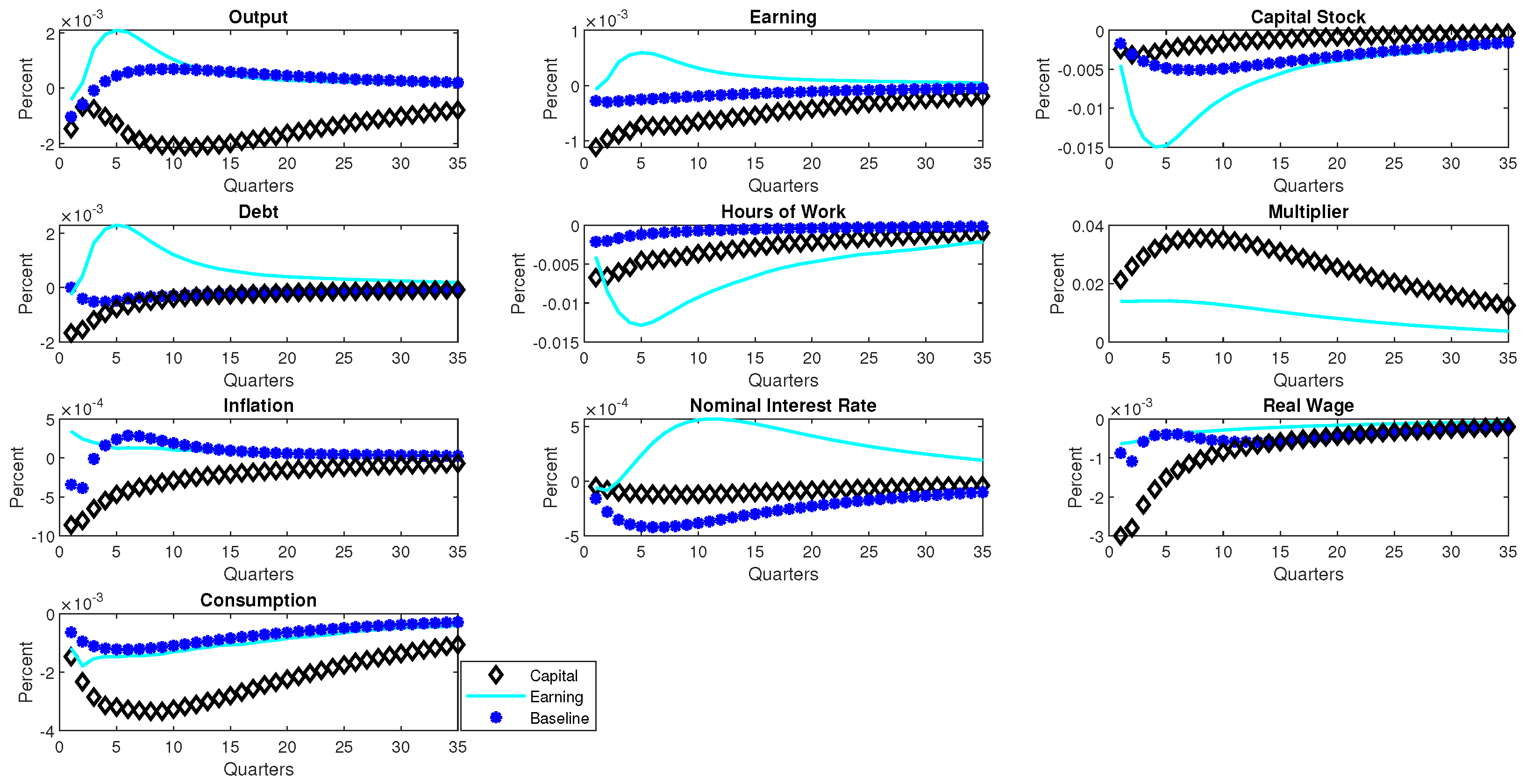
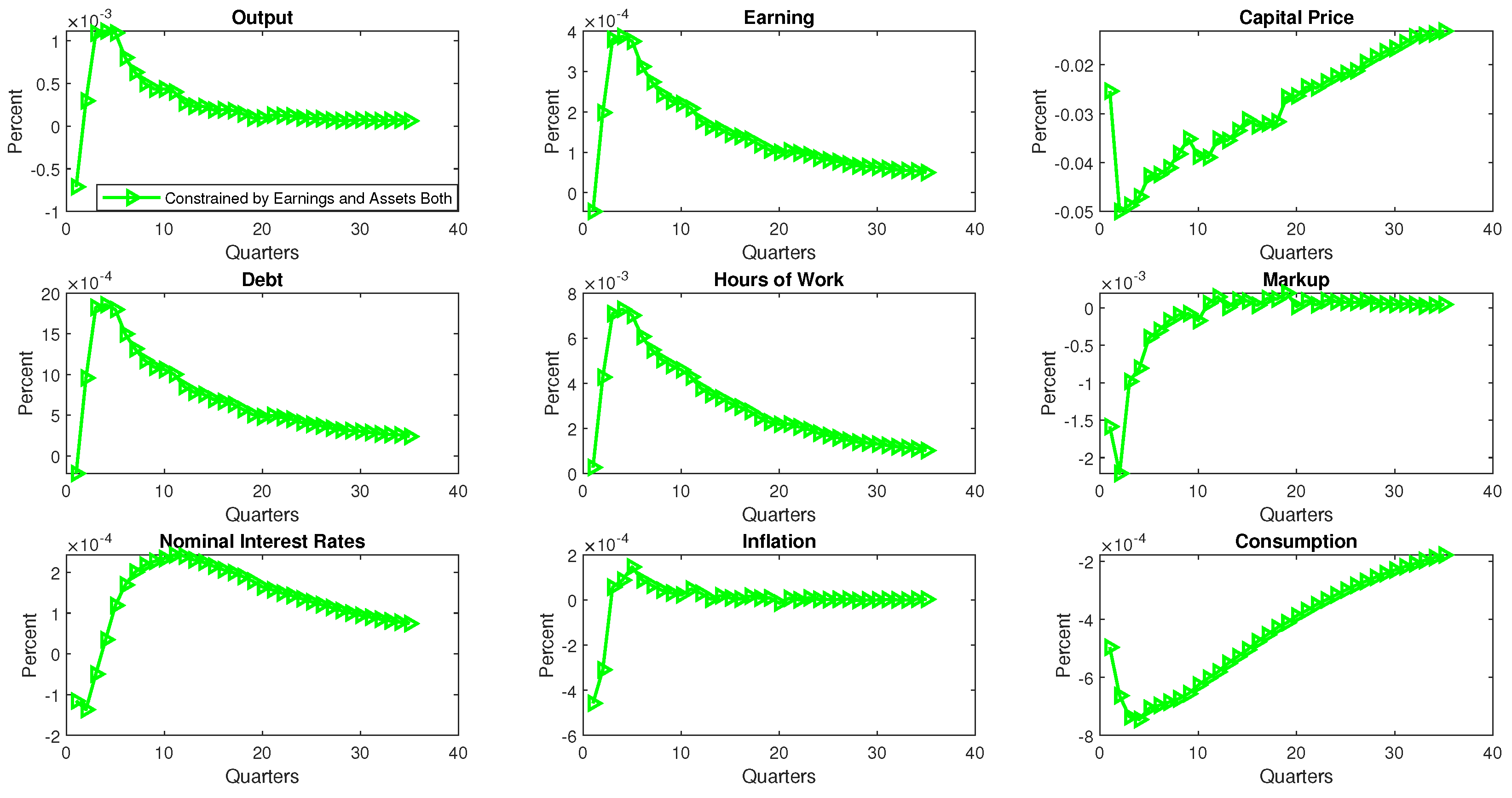
where p is the probability that the loan is backed by earnings, and ( 1 p ) is the probability that the loan is backed by assets. Since we could not find data on corporate loans that are backed by both earnings and capital simultaneously, we rely on the findings by Lian and Ma (2020). We therefore set the p = 0.8 , assuming that a firm, constrained by both earnings and capital, is 80% likely to pledge its earnings for acquiring credit. Figure 5 reports the impulse responses of selected variables for this case.
In this analysis, we focus more on the cyclical properties of output, inflation and the price markup to see how they compare with the data (VAR model). The results are particularly interesting. First, following the rise in uncertainty, both output and inflation decline in the first few quarters, which is an indication that the demand side effects dominate that of the supply side. This is consistent with the results in the VAR model. Secondly, the price markup falls (concurrently with output) in response to the shock. In this regard, the price markup is procyclical, with the correlation coefficient between the simulated output and the markup estimated to be about 0.50. This is also in line with the results in the VAR analysis (where the correlation is estimated to be about 0.12). This outcome is perhaps due to the competing effects of the shock on output, which in turn affects the tightness in the borrowing constraint in the case of the earnings based constraint: Under the asset-based constraint, the firm has the incentive to produce at a significantly lower level, as doing so would lead to an increase in the markup. In the case of the earnings-based constraint however, the firm guards against the decline in output (and revenue), since that would lead to a decline in credit worthiness, and for that matter a tighter credit market.
One weakness arising from this formulation rests on the behavior of the hours of work which rises in response to uncertainty shocks contrary to the results in the VAR model. Notwithstanding, the findings show that the nature and form of the borrowing constraint is important in determining how we characterize uncertainty shocks in the economy which we hope would provide further insight into the understanding of this subject as it relates to macroeconomic fluctuations

5. Summary and Conclusions

This paper explores the role of the credit channel of uncertainty shocks in driving macroeconomic conditions in the US economy. In the quantitative literature, uncertainty shocks are shown, in general, to exhibit properties of a negative demand shock (see for example Leduc and Liu 2016). To this extent, uncertainty shocks propagate in the economy through a counter cyclical markup channel if prices are sufficiently sticky. In our set up, we model borrowing constraints as a nested function that features both corporate earnings and capital as alternative instruments for assessing credit worthiness in the corporate sector, in line with recent trends in corporate finance. This particular design allows us to analyze the macroeconomic effects of uncertainty shocks under alternative credit market settings: in one setting, borrowing is backed by the value of capital; in another setting, borrowing is tied exclusively to corporate earnings. We also extend the analysis to look at a hybrid scenario where borrowing is tied to both corporate earnings and the value of capital stock. In a preliminary analysis, we motivate the study by examining the effects of uncertainty shocks on the US economy using a Vector Auto-Regressive (VAR) model.
We find that the quantitative framework that incorporates only one instrument (capital or earnings) in the borrowing constraint falls short in matching the business cycle properties of the US economy (in the VAR model) in terms of the behavior of output, inflation, and the price markup which are an essential part of the literature on uncertainty shocks. Rather, a hybrid formulation of the borrowing constraint which accounts for both capital and earnings helps us bring the results in the quantitative model closer to the data. Specifically, the price level falls alongside output in the model with capital-based constraint, but rises in the model with earnings-based constraint. To this end, the uncertainty shock displays properties of a demand side shock in the presence of the asset-based constraints. The opposite is true in the case of the model with earnings-based constraint. In addition, following the rise in uncertainty, the price markup is countercyclical in the presence of the asset-based borrowing constraints. However, it becomes procyclical in the model with earnings-based borrowing constraint. In a special case with a hybrid formulation of the borrowing constraint where both capital and earnings are concurrently used as instruments for assessing credit worthiness, the results improve upon that of the other models in which borrowing is constrained by only one instrument (assets or earnings)—by matching the cyclical properties of output, prices and the mark-up in the VAR model. In this specification, the shock exhibits properties of a demand side shock which matches the data. Additionally, the price mar-up is procyclical, which is also consistent with the data.
The above findings show that alternative formulations of borrowing constraints matter for the propagation of second-moment shocks in the DSGE model. The paper contributes to the plethora of literature on the effects of uncertainty shocks in the economy. However, it departs from the rest of the literature by formulating and incorporating credit frictions in a unique way, which we hope would provide further insight into the understanding of uncertainty shocks and macroeconomic fluctuations.
Author Contributions

Conceptualization, A.K. and N.P.K.; methodology, A.K. and N.P.K.; software, A.K. and N.P.K.; validation, A.K. and N.P.K.; formal analysis, A.K. and N.P.K.; investigation, A.K. and N.P.K.; resources, A.K. and N.P.K.; data curation, A.K. and N.P.K.; writing—original draft preparation, A.K. and N.P.K.; writing—review and editing, A.K. and N.P.K.; visualization, A.K. and N.P.K. All authors have read and agreed to the published version of the manuscript.

Funding

This research received no external funding.

Informed Consent Statement

Not applicable.

Data Availability Statement

Data is sourced from the Febral Reserve Bank of St. Louis. https://fred.stlouisfed.org/ (accessed on 5 December 2021).

Conflicts of Interest

The authors declare no conflict of interest.

Appendix A. Empirical Section

Appendix A.1. Data Construction for VAR Model Estimation

Sources of Data: Data used in the empirical analysis come from a number of sources, including the National Income and Product Account (NIPA), Bank of International Settlements (BIS), and the Federal Reserve Bank of St. Louis. In construction of the the relative price of investment data, we followed the procedure by Drechsel (2020). Table A1 explains data construction process.
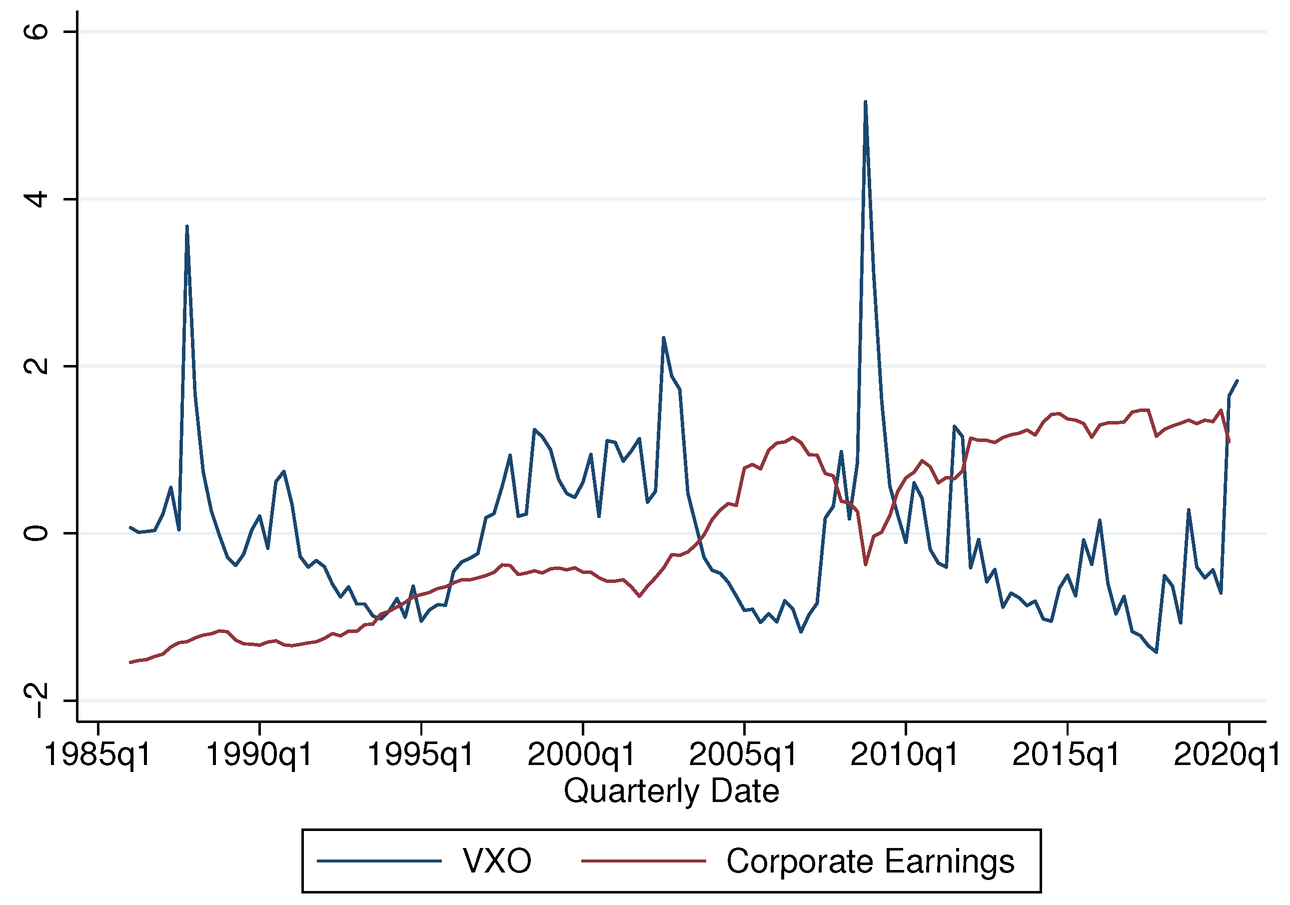
Details on Corporate Earnings: For corporate earnings, We use the item ’Corporate Business Profits before tax, without IVA and CCAdj’ from the FRED website. Figure A1 below shows the time-series of earnings thus constructed along with the proxy of uncertainty.
Details on Capital Stock: For capital stock, on the other hand, we take the item’ Total Capital Expenditures, Flow’ is from the FRED website. Figure A2 below shows the time-series of capital stock constructed along with the VXO.
Figure A1. Corporate Earnings and the VXO. Notes: The figure shows the time-series of the corporate sector earnings along with the proxy of uncertainty. The figure suggests that corporate earning is procyclical while the uncertainty proxy is countercyclical. The correlation coefficients between the VXO and firms’ earning is −0.30. Both series are normalized.
Ijfs 11 00021 g0a1
Figure A2. Capital Stock and the VXO. Notes: The figure shows the time-series of the corporate sector earnings along with the proxy of uncertainty. The figure suggests that capital stock is procyclical while the uncertainty proxy is countercyclical. The correlation coefficients between the VXO and firms’ earning is −0.21. Both series are normalized.
Ijfs 11 00021 g0a2
Table A1. Construction of Variables used in the Empirical Analysis.
VariablesSources and Data ConstructionData Transformation
Price LevelConsumption Deflator (FRED: CONSDEF)log
GDPReal Gross Domestic Product (FRED: GDPC1)log
VXOCBOE S&P 100 Volatility Index (FRED: VXOCLS)log
Business Sector EarningsSum of Corporate Business Profits before tax, without IVA and CCAdj (FRED: A446RC1Q027SBEA) and
Non-financial Income before taxes, flow (FRED: BOGZ1FA146110005Q), deflated with consumption deflator.
log
Level of Capital StockDomestic Nonfinancial Sectors; Total Capital Expenditures, Flow (FRED:BOGZ1FA385050005Q) minus
Nonfinancial Corporate Business; Consumption of Fixed Capital, Structures, Equipment,
and Intellectual Property Products, Including Equity REIT Residential Structures (NIPA Basis), Flow
(FRED: BOGZ1FA106300003Q), valued at the relative price of investment.
log
Credit Flow to Non-Financial Corporate SectorCredit to Private non-financial sector from All sectors at Market value, deflated with consumption deflator (BIS).log
Relative Price of InvestmentImplicit Price Deflators, Nonresidential, Equipment, Fixed Investment (FRED: Y033RD3Q086SBEA),
deflated with Consumption Deflator (CONSDEF)
log
Economic Policy Uncertainty Index (EPUI)Uncertainty Proxy for Robustness Analysis. Collected from https://www.policyuncertainty.com/ (accessed on 6 November 2021).log
Hours WorkedNonfarm Business Sector: Hours of All Persons (FRED: HOANBS)log
Interest RateEffective Federal Funds (FRED:DFF)
Interest Rate (Robustness Check)Wu-Xia Shadow Rate. Collected from https://sites.google.com/view/jingcynthiawu/shadow-rates (accessed on 6 November 2021).
Business Sector ConfidenceBusiness Tendency Survey, Confidence Indicator for United States (FRED: BSCICP03USM665S)log
MarkupWages and Salaries’ component of Personal Income (NIPA) Divided by Real GDP (GDPC1), Inverselog

Appendix A.2. Using the Economic Policy Uncertainty Index (EPUI)

Figure A3. The Effects of Uncertainty Shocks when Economic Policy Uncertainty Index (EPUI) is used as a Proxyy. Notes: Figure A3 shows the effect of one standard deviation increase in EPUI on the US output, Hours, Credit Flow to Non-financial Corporates, Firms’ Capital Stock, Firms’ Earning, the Relative Price of Investment, and markup. In the impulse response functions, the shades represent the one standard deviation confidence interval while the middle bold line represents the median response of variables due to uncertainty increase. The data are quarterly and span the period 1986Q1-2019Q4. In the VAR model, all the variables are in log levels, with the exception of the federal funds rate.
Ijfs 11 00021 g0a3

Appendix A.3. Using the Nekarda and Ramey (2021) Measure of the Price Mark-Up

Figure A4. The Effects of Uncertainty Shocks when the Nekarda and Ramey (2021) Measure of the Price Mark-Up is Used. Notes: Shaded regions represent 90 percent standard error bands. The data are quarterly and span the period 1986Q1-2019Q4. With the exception of the federal funds rate, all the other variables are in log levels. The figure shows that both the output and markup decrease following an increase in uncertainty.
Ijfs 11 00021 g0a4

Appendix A.4. Changes in the Ordering of the Price Mark-Up

In this part, we re-estimate the VAR model after changing the order of variables. The new orderings is as follows:
( V A R 10 ) = Measure   of   uncertainty Markup Relative   Price   of   Investment GDP   Deflator Hours   of   Work Capital   Stock   of   Non financial   Corporate   Sector Earnings   of   Non Financial   Corporate   Sector Credit   Flow   to   Non financial   Corporate   Sector Output Federal   Funds   Rate
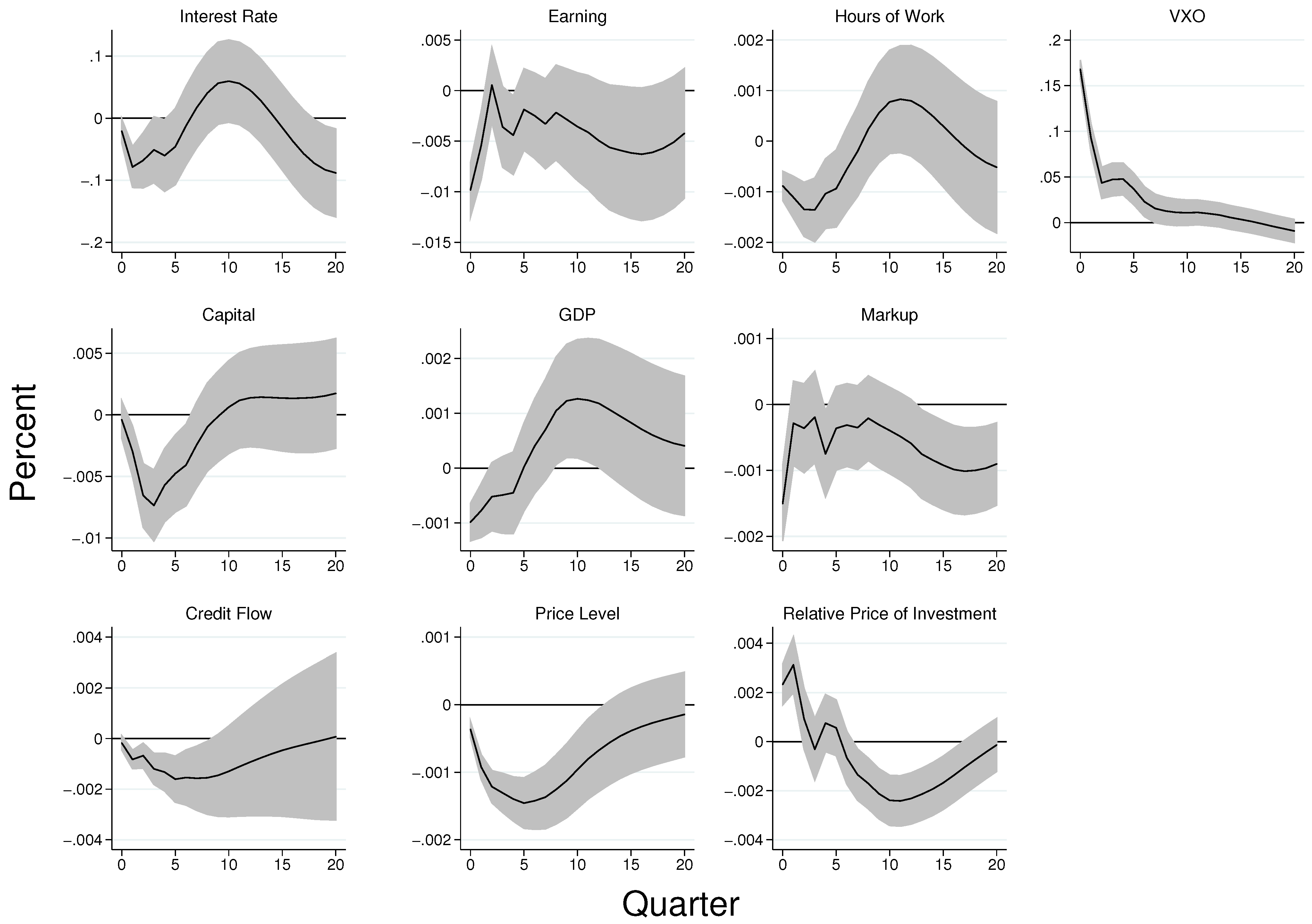
Figure A5 presents the results. In the figure, we can see that markup and output both decrease following an increase in uncertainty shock, making the markup procyclical. The result suggests that pro-cyclical nature of markup obtained from earnings-based constraints in the DSGE model is likely to match some key features in the data.
Figure A5. Effect of Uncertainty Shocks under Different Ordering of Variables. Notes: Shaded regions represent 90 percent standard error bands. The data are quarterly and span the period 1986Q1-2019Q4. With the exception of the federal funds rate, all the other variables are in log levels. The figure shows that output and markup decrease following an increase in uncertainty. Moreover, the correlation coefficient between simulated output and markup after uncertainty shock is computed to be 0.11, making markup procyclical.
Ijfs 11 00021 g0a5

Appendix A.5. Using the Wu-Xia Shadow Rate as a Proxy for Monetary Policy

Figure A6. Uncertainty Shock Effects on the US Economy when Wu-Xia Shadow Rate is Used as a Proxy of Monetary Policy. Notes: Figure A6 shows the effect of one standard deviation increase in the VXO on the US output, Hours, Credit Flow to Non-financial Corporates, Firms’ Capital Stock, Firms’ Earning, and the Relative Price of Investment. In the impulse response functions, the shades represent the 90% confidence interval while the middle bold line represents the median response of variables due to uncertainty increase. The data are quarterly and span the period 1986Q1-2019Q4. In the VAR model, all the variables are in log levels, with the exception of the federal funds rate.
Ijfs 11 00021 g0a6

Appendix A.6. Uncertainty Shocks and Business Confidence

( V A R 10 ) = Measure   of   uncertainty Business   Confidence Relative   Price   of   Investment GDP   Deflator Hours   of   Work Capital   Stock   of   Non financial   Corporate   Sector Earnings   of   Non Financial   Corporate   Sector Credit   Flow   to   Non financial   Corporate   Sector Real   GDP Federal   Funds   Rate
Figure A7. Uncertainty Shocks and Business Confidence. Notes: Shaded regions represent 95 percent standard error bands. The data are quarterly and span the period 1986Q1-2019Q4. With the exception of the federal funds rate, all the other variables are in log levels.
Ijfs 11 00021 g0a7

Appendix A.7. Effect of Uncertainty Shocks When Non-Uncertainty Variables Are Ordered First

Figure A8. Effects of Uncertainty Shocks when Non-Uncertainty Variables are Ordered First. Notes: This figure shows the effect of one standard deviation increase in the VXO on the US output, Hours, Credit Flow to Non-financial Corporates, Firms’ Capital Stock, Firms’ Earning, and the Relative Price of Investment. The ordering of variables is as follows: relative price of investment, price level, hours of work, VXO, capital stock, firms’ earning, credit flow to non-financial sector, GDP, and the federal funds rate. In the impulse response functions, the shades represent the 90% confidence interval while the middle bold line represents the median response of variables due to uncertainty increase. The data are quarterly and span the period 1986Q1-2019Q4. In the VAR model, all the variables are in log levels, with the exception of the federal funds rate.
Ijfs 11 00021 g0a8

Appendix B. Effects of Uncertainty Shocks in a DSGE Model

Appendix B.1. Steady State Equations

In the steady state expectation operators are removed and variables are written in such a way that x t + 1 = x t = x . Additionally exogenous processes are absent. From (5), we obtain the solution for the interest rates (R)
R = π β
The production function in steady state is written as
Y N = A K N α
From Equation (11), we can obtain the relation between investment and capital as follows:
I = δ K
From the price Phillips curve Equation (18), we obtain a relationship between the marginal cost of production (mc) and the multiplier on the credit constraint equation
ε 1 = ε m c ( ϵ 1 ) θ π E p μ
Expression of wage obtained from the first order condition of the production sector can be written as:
w = ( 1 α ) A ( K N ) α m c 1 + μ θ π E
From the first order condition of firm’s profit with respect to investment, we obtain:
q = 1 + μ
From Equation (17), we obtain an expression of the capital–labor ratio as follows:
K N = α A m c 1 β ( 1 δ ) μ θ k ( 1 p ) 1 1 α
Collateral constraint in steady state in steady equation is given as follows:
I = p π θ π E + ( 1 p ) θ k q K
Earnings are expressed as:
π E = y w n
Resource constraint becomes:
y = c + i
Based on the relationship between investment and capital and given the resource constraint, consumption per capita can be written as:
c N = A K N α δ K N
From labor supply Equation (6), we can obtain an expression for N as follows:
N = λ w χ 1 ν
Non-linear solution of Equations (29)–(40) gives the steady state values of endogenous variables in all the three cases. Calibration of parameters used for steady state calculation of variables are described in the next subsection.

Appendix B.2. Demand Uncertainty Shocks and Borrowing Constraints

In the foregoing analysis, we looked at the business cycle properties of second moment shocks total factor productivity. In this section, we look at the effects of a demand side uncertainty shock. The goal is to see if the origin of uncertainty matters for the resultant business cycle properties. To conduct this analysis, we assume that the standard deviation of household preferences is time-varying in nature. Specifically, we assume that household preferences evolve as follows:
l o g γ t = ( 1 ρ γ ) l o g γ + ρ γ l o g γ t 1 + σ t 1 D η t .
where σ t D follows an AR(1) process as follows:
σ t D = ( 1 ρ σ D ) l o g σ D + ρ σ D l o g σ t 1 D + σ σ t D η t p ,
with ρ σ D being the persistence parameter of second-moment household preference shock. σ σ t D is the standard deviation of the second moment shock, and lastly η t p is a shock to the demand uncertainty. The results are shown in Figure A9.
The qualitative aspects of difference in uncertainty effects remain valid even when uncertainty shock in demand side is considered. In particular, following an increase in uncertainty shock, earnings, and the value of the capital stock of the non-financial sector decreases, making difficult for firms to access external debt, affecting overall macroeconomic variables such as output and inflation negatively. Those results remain valid in the models with alternative measurements of frictions. The divergence between the frictions in terms of the markup, as observed in Section 4.2.1, still exists. As a result, both the real variables and inflation encounter weak uncertainty effects in the model with earnings-based restrictions relative to assets-based ones. The detailed economic impact of demand uncertainty shocks across both measures of frictions can be found in Appendix B.3.
Figure A9. Effects of Demand Uncertainty Shocks in a DSGE Model with Alternative Formulations of Borrowing Constraints. Notes: Figure A9 shows the impulse responses of macroeconomic variables to a standard deviation shock in demand uncertainty, when different measurements of credit frictions are used. The black lines represent the responses of the model with asset-based constraints while the cyan colored lines are outcome of earnings-based constraints. The structural parameters to generate these IRFs are shown in Table 2. We calculate ρ σ D = 0.4 and σ σ t D = 0.058 .
Ijfs 11 00021 g0a9

Appendix B.3. Uncertainty Shocks at the Zero Lower Bound (ZLB) in a DSGE Model

For the DSGE model, we simulate the DSGE model explained above, considering that the nominal interest rate binds indefinitely. That can be conducted by setting R t = 1 + r t in the monetary policy Equation (24) where r t is the net interest rate. To implement the ZLB in Dynare, we set r t = 0 during the simulation. Figure A10 presents the results. In the figure, the cyan colored lines show the responses of the model with earnings-based borrowings. The black-colored line shows the impacts in the model with assets-based borrowing constraints.
The results suggests that the uncertainty shock decreases corporate earnings and the value of capital stock, which hinders firms’ access to external credit. This leads to a decline in output, hours of work, and real wage of workers. The multiplier ( μ ) on the borrowing constraints increases regardless of the form of the borrowing constraint, which signifies tightening in the credit market. This is consistent with the findings in the main models (in normal times). One point of departure from the non-ZLB condition is that inflation declines in the model with earnings-based borrowing constraints when the ZLB is binding. The decline in inflation under both formulation of the borrowing constraint might explain the behavior of inflation during the great recession of 2008/09 in which the nominal interest rate was kept very low for an extended period of time. However, the decline in inflation is lower with the earnings-based borrowing constraints than that of assets-based borrowing constraints, which might be explained by the weakly procyclical markup in the model with earnings-based constraint.
Figure A10. Impulse Responses at the ZLB When Earning-Based Constraints Are Binding. Notes: The figure displays model IRFs of different model variables to technology uncertainty shocks when the nominal interest rate is subjected to the Zero Lower Bound infinitely, under two alternative calibrations in which only the earnings-based constraint (cyan colored lines) or only the assets-based constraint (black colored lines) is present. The structural parameters to generate these IRFs are shown in Table 2. Based on a VAR analysis (not shown), we calculate ρ σ = 0.0122 and σ σ t A = 0.063.
Ijfs 11 00021 g0a10

Appendix B.4. Effects of First Moment Shocks on Credit Dynamics

In this subsection, we explore the effects of a first moment total factor productivity shock in the economy. Figure A11 plots impulse responses of selected variables to one standard deviation increase in the TFP. In the figure, the cyan colored lines correspond to the model in which firms face earnings-based borrowing constraints, while the impulses with black diamonds are generated with asset-based collateral constraints. Lastly, the impulses with blue stars correspond to the outcomes from the model without credit constraints.
As expected, the TFP shock generates stimulative effects in the economy as evidenced by the behavior the selected variables. In addition, this is true regardless of whether the model features borrowing constraints or not. In addition, it is shown that the multipliers ( μ ) decline under both formulations of the borrowing constraints in the wake of the shock, which signifies loosening of the credit market. This is contrary to the outcome under the second moment shock. It is also shown that, although output rises in all cases, it is less so on impact under the two models that feature borrowing constraints, which is also expected. Following the rise in output, earnings and capital also rise more under the baseline model relative to the model with credit constraints.
Figure A11. Technology Shock, Earning-Based Borrowing Constraints, and Credit Dynamics. Notes: Figure A11 displays model IRFs of different model variables to technology shocks, under three alternative calibrations in which only the earnings-based constraint (cyan colored lines), only the collateral constraint (lines with black diamonds), or without any constraints (impulses with blue stars) is present. The parameters to generate these IRFs are shown in Table 2. We set ρ A = 0.95 and σ A = 0.01.
Ijfs 11 00021 g0a11

Notes

1
2

References

  1. Abel, Andrew B. 1983. Optimal Investment under Uncertainty. American Economic Review 73: 228–33. [Google Scholar]
  2. Adjemian, Stephane, Houtan Bastani, Michel Juillard, Fredrick Karame, Ferhat Mihoubi, George Perendia, Johannes Pfeifer, Marco Ratto, and Sebastien Villemot. 2011. Dynare Reference Manual, Version 4. Available online: https://www.dynare.org/wp-repo/dynarewp001.pdf (accessed on 10 February 2022).
  3. Aghion, Phillip, George M. Angeletos, Abhijit Banerjee, and Kalina Manova. 2010. Volatility and growth: Credit Constraints and the Composition of Investment. Journal of Monetary Economics 57: 246–65. [Google Scholar] [CrossRef] [Green Version]
  4. Auerbach, Alan J., and Yuriy Gorodnichenko. 2012. Measuring the Output Responses to Fiscal Policy. American Economic Journal: Economic Policy 4: 1–27. [Google Scholar] [CrossRef] [Green Version]
  5. Baker, Scott. R., Nicholas Bloom, and Steven J. Davis. 2016. Measuring Economic Policy Uncertainty. The Quarterly Journal of Economics 131: 1593–636. [Google Scholar] [CrossRef]
  6. Balke, Nathan S., Enrique Martínez-García, and Zheng Zeng. 2017. Understanding the Aggregate Effects of Credit Frictions and Uncertainty. Working Paper No. 317. Dallas: Federal Reserve Bank of Dallas. [Google Scholar]
  7. Bansal, Ravi, and Amir Yaron. 2004. Risks for the Long Run: A Potential Resolution of Asset-Pricing Puzzles. The Journal of Finance 4: 1481–509. [Google Scholar] [CrossRef] [Green Version]
  8. Basu, Susanto, and Brent Bundick. 2017. Uncertainty Shocks in a Model of Effective Demand. Econometrica 85: 937–58. [Google Scholar] [CrossRef] [Green Version]
  9. Begley, Joy. 1994. Restrictive Covenants Included in Public Debt Agreements: An Empirical Investigation. Working Paper. Vancouver: University of British Columbia. [Google Scholar]
  10. Bernanke, Ben S. 1983. Irreversibility, uncertainty, and cyclical investment. Quarterly Journal of Economics 98: 85–106. [Google Scholar] [CrossRef] [Green Version]
  11. Benmelech, Efraim, Nittai Kumar, and Raghuram Rajan. 2020. The Decline of Secured Debt. NBER Working Paper 26637. Cambridge: NBER. [Google Scholar] [CrossRef]
  12. Bernanke, Ben S., Mark Gertler, and Simon Gilchrist. 1999. Chapter 21 The financial accelerator in a quantitative business cycle framework. In Handbook of Macroeconomics. New York: Elsevier, Vol. 1, pp. 1341–93. ISBN 9780444501585. [Google Scholar] [CrossRef]
  13. Bloom, Nicholas. 2009. The Impact of Uncertainty Shocks. Econometrica 77: 623–85. [Google Scholar]
  14. Bordo, Michael D., John V. Duca, and Christoffer Koch. 2016. Economic Policy Uncertainty and the Credit Channel: Aggregate and Bank Level U.S. Evidence Over Several Decades. NBER Working Paper 22021, NBER, Cambridge. Available online: http://www.nber.org/papers/w22021 (accessed on 10 February 2022).
  15. Born, lBenjamin, and lJohannes Pfeifer. 2014. Policy risk and the business cycle. Journal of Monetary Economics 68: 68–85. [Google Scholar] [CrossRef] [Green Version]
  16. Bradley, Michael, and Michael R. Roberts. 2015. The Structure and Pricing of Corporate Debt Covenants. Quarterly Journal of Finance 5: 1–37. [Google Scholar] [CrossRef]
  17. Brand, Thomas, Marlene Isore, and Fabien Tripier. 2019. Uncertainty shocks and firm creation: Search and monitoring in the credit market. Journal of Economic Dynamics and Contorl 99: 19–53. [Google Scholar] [CrossRef] [Green Version]
  18. Carriero, Andrea, Haroon Mumtaz, Konstatinos Theodoridis, and Angeliki Theophilopoulou. 2015. The Impact of Uncertainty Shocks under Measurement Error: A Proxy SVAR Approach. Journal of Money, Credit, and Banking 47: 1221–38. [Google Scholar] [CrossRef] [Green Version]
  19. Cesa-Bianchi, Ambrogio, and Emilio Fernandez-Corugedo. 2018. Uncertainty, Financial Frictions, and Nominal Rigidities: A QUantitative Investigation. Journal of Money, Credit, and Banking 50: 603–36. [Google Scholar] [CrossRef] [Green Version]
  20. Choi, Sangyup, Davide Furceri, Yi Huang, and Prakash Loungani. 2018. Aggregate uncertainty and sectoral productivity growth: The role of credit constraints. Journal of International Money and Finance 88: 314–30. [Google Scholar] [CrossRef] [Green Version]
  21. Crouzet, Nicolas. 2017. Aggregate implications of corporate debt choices. Review of Economic Studies 85: 1635–82. [Google Scholar] [CrossRef]
  22. De Fiore, Fiorella, and Herald Uhlig. 2011. Bank finance versus bond finance. Journal of Money, Credit, and Banking 43: 1399–421. [Google Scholar] [CrossRef] [Green Version]
  23. Donaldson, Jason R., Denis Gromb, and Georgia Piacentino. 2020. Conflicting Priorities: A Theory of Covenants and Collateral. 2019 Meeting Papers No 157. Cartegena: Society for Economic Dynamics. [Google Scholar]
  24. Drechsel, Thomas. 2020. Earning-Based Borrowing Constraints and Macroeconomic Fluctuations. New York: Mimeo. [Google Scholar]
  25. Fernandez-Villaverde, Jesus, Pablo A. Guerron-Quintana, Juan F. Rubio-Ramirez, and Martin Uribe. 2011. Risk Matters: The Real Effects of Volatility Shocks. The American Economic Review 101: 2530–61. [Google Scholar] [CrossRef] [Green Version]
  26. Frank, Murrry Z., and Vidhan K. Goyal. 2009. Capital structure decisions: Which factors are reliably important? Financial Management 38: 1–37. [Google Scholar]
  27. Gilchrist, Simon, Jae W. Sim, and Egon Zakrajsek. 2017. Uncertainty, Financial Frictions, and Investment Dynamics. NBER Working Paper 20038. Cambridge: National Bureau of Economic Research, Inc. [Google Scholar]
  28. Hartman, Richard. 1972. The effects of price and cost uncertainty on investment. The Journal of Economic Theory 5: 258–66. [Google Scholar] [CrossRef]
  29. Holmstrom, Bengt, and Jean Tirole. 1997. Financial Intermediation, Loanable Funds, and the Real Sector. The Quarterly Journal of Economics 112: 663–91. [Google Scholar] [CrossRef]
  30. Ireland, Peter N. 2007. Changes in the Federal Reserve’s Inflation Target: Causes and Consequences. Journal of Money, Credit, and Banking 39: 1851–82. [Google Scholar] [CrossRef]
  31. Ivashina, Victoria, Luc Laeven, and Enrique M. Benito. 2020. Loan Types and Bank Lending Channel. Working Paper. Madrid: Bank of Spain. [Google Scholar]
  32. Jermann, Urban, and Vincenzo Quadrini. 2012. Macroeconomic Effects of Financial Shocks. American Economic Review 102: 238–71. [Google Scholar] [CrossRef] [Green Version]
  33. Kermani, Amir, and Yueran Ma. 2020. Two Tales of Debt. NBER Working Paper 27641. Cambridge: National Bureau of Economic Research. [Google Scholar] [CrossRef]
  34. Kiyotaki, Nobuhiro, and John Moore. 1997. Credit Cycles. Journal of Political Economy 105: 211–48. [Google Scholar] [CrossRef]
  35. Leduc, Sylvian, and Keith Sill. 2007. Monetary Policy, Oil Shocks, and TFP: Accounting for the Decline in U.S. Volatility. Review of Economic Dynamics 10: 595–614. [Google Scholar] [CrossRef] [Green Version]
  36. Leduc, Sylvian, and Keith Sill. 2013. Expectations and Economic Fluctuations: An Analysis Using Survey Data. The Review of Economics and Statistics 95: 1352–67. [Google Scholar] [CrossRef]
  37. Leduc, Sylvia, and Zheng Liu. 2016. Uncertainty Shocks are Aggregate Demand Shocks. Journal of Monetary Economics 82: 20–35. [Google Scholar] [CrossRef] [Green Version]
  38. Lian, Chen, and Yueran Ma. 2020. Anatomy of corporate borrowing constraints. The Quarterly Journal of Economics 136: 229–91. [Google Scholar] [CrossRef]
  39. Lutkepohl, Helmut. 2005. New Introduction to Multiple Series Analysis. Berlin: Springer. [Google Scholar]
  40. Malitz, Ileen. 1986. On Financial Contracting: The Determinants of Bond Covenants. Financial Management 15: 18–25. [Google Scholar] [CrossRef]
  41. Mendoza, Enrique G. 2010. Sudden Stops, Financial Crises, and Leverage. American Economic Review 100: 1941–66. [Google Scholar] [CrossRef]
  42. Mumtaz, Haroon, and Paolo Surico. 2018. Policy uncertainty and aggregate fluctuations. Journal of Applied Econometrics 33: 319–31. [Google Scholar] [CrossRef]
  43. Nekarda, Christopher J., and Valleri A. Ramey. 2021. The Cyclical Behavior of the Price-Cost Markup. Journal of Money Credit and Banking 52: 319–53. [Google Scholar] [CrossRef]
  44. Oi, Walter Y. 1961. The desirability of price instability under perfect competition. Econometrica 29: 58–64. [Google Scholar] [CrossRef]
  45. Rauh, Joshua D., and Amir Sufi. 2010. Capital Structure and Debt Structure. The Review of Financial Studies 23: 4242–280. [Google Scholar] [CrossRef] [Green Version]
  46. Roberts, Michael R., and Amir Sufi. 2009. Renegotiation of financial contracts: Evidence from Private Credit Agreements. Journal of Financial Economics 93: 159–84. [Google Scholar] [CrossRef]
  47. Rotemberg, Julio J. 1982. Sticky Prices in the United States. Journal of Political Economy 90: 1187–211. [Google Scholar] [CrossRef] [Green Version]
  48. Smets, Frank, and Rafael Wouters. 2007. Shocks and Frictions in U.S. Business Cycles: A Bayesian DSGE Approach. American Economics Review 97: 586–606. [Google Scholar] [CrossRef] [Green Version]
  49. Smith, Clifford W., and Jerold B. Warner. 1979. On Financial Contraction: An Analysis of Bond Covenants. Journal of Financial Economics 7: 117–61. [Google Scholar] [CrossRef]
  50. Stiglitz, Joseph E., and Andrew Weiss. 1981. Credit Rationing in Markets with Imperfect Information. The American Economic Review 71: 393–410. [Google Scholar]
  51. Valencia, Fabian. 2017. Aggregate Uncertainty and the Supply of Credit. Journal of Banking and Finance 81: 150–65. [Google Scholar] [CrossRef] [Green Version]
  52. Wu, Jing C., and Fan D. Xia. 2016. Measuring the Macroeconomic Impact of Monetary Policy at the Zero Lower Bound. Journal of Money, Credit, and Banking 48: 253–91. [Google Scholar] [CrossRef]
Figure 1. Time-Series of the VXO from 1986Q1 to 2020Q1.
Ijfs 11 00021 g001
Figure 2. Impulse Responses to Uncertainty Shock in the VAR Model. Notes: Shaded regions represent 95 percent standard error bands. The data are quarterly and span the period 1986Q1-2019Q4. With the exception of the federal funds rate, all the other variables are in log levels.
Ijfs 11 00021 g002
Figure 3. Impulse Responses to a productivity Uncertainty Shock Under Alternative Borrowing Constraints. Notes: The Figure presents the model IRFs of selected variables to a productivity uncertainty shocks. The cyan colored lines represent the model with earnings-based constraint, the black diamonds represent the model with asset-based constraints, whereas the responses with blue stars represent the baseline model without any financial frictions. The parameter sets that generate the IRFs are presented in Table 2. In addition, we set ρ σ = 0.4 and σ σ t A = 0.058.
Ijfs 11 00021 g003
Figure 4. Impulse Responses of the Price Markup to a Productivity Uncertainty Shock under Alternative Borrowing Constraints. Notes: The figure displays model IRFs of the markup to a productivity uncertainty shock. The cyan colored lines represent the model with earnings-based constraint, the black diamonds represent the model with asset-based constraints, whereas the responses with blue stars represent the baseline model without any financial frictions. The parameter sets that generate the IRFs are presented in Table 2. In addition, we set ρ σ = 0.4 and σ σ t A = 0.058.
Ijfs 11 00021 g004
Figure 5. Impulse Responses to Uncertainty Shocks When Both Asset and Earnings Based Constraints are Binding. Notes: The figure displays the model IRFs of selected variables to productivity uncertainty shocks when borrowing by the corporate sector is constrained by both earnings and assets. The parameters to generate these IRFs are shown in Table 2. To obtain the IRFs we estimate ρ σ = 0.4 and σ σ t A = 0.058.
Ijfs 11 00021 g005
Table 1. Share of Asset Based Lending vs. Earnings-Based Covenant.
PapersShare of
Assets-Based
Loans (%)
Share of
Earnings-Based
Loans (%)
Share of Loans
Backed by
Both (%)
Information
Unavailable (%)
Sample Size
Firms
Rauh and Sufi (2010)6.524.713.255.62453 firms
Lian and Ma (2020)2080 58,241 (Cash-Based loans)
58,227 (Assets-Based loans)
Drechsel (2020)3035 3550,000 loan deals
(15,000 firms)
Ivashina et al. (2020)41.851.7
Notes: Weights in Rauh and Sufi (2010 are calculated based on the classifications by Lian and Ma (2020). Mortgages are assets-based. Bonds are mostly cash based. Loans without a fixed number of payments (revolvers) and monetary loans that have regular payments over a period of time (term-loans) are backed by cash and assets.
Table 2. Summary of Parameters for the Benchmark Analysis in the DSGE Model.
ParameterDescriptionValue
Structural Parameters
β Hoursehold’s Discount Factor0.99
χ Disutility of Work0.564
ψ Price Adjustment Cost110
π Inflation Target1.0045
Ψ π Policy Weight on Inflation1.5
Ψ R Persistence of Interest Rate0.9
Ψ y Policy Weight on Output0.125
Φ Capital Adjustment Cost2
ρ Probability of Debt being Backed by Earnings1
α Output Elasticity of Capital0.33
ν Elasticity of Labor Supply1
ϵ Price Elasticity of Demand6
θ k Loan to Value Ratio0.067
θ π Loan to Earnings Ratio5.77
NSteady State Work0.33
Shock Process
ρ A Persistence of Technology Shock0.95
ρ σ Persistence of Shock to Volatility of Technology Shock0.4
σ σ t A Volatility of Uncertainty Shock0.058
Disclaimer/Publisher’s Note: The statements, opinions and data contained in all publications are solely those of the individual author(s) and contributor(s) and not of MDPI and/or the editor(s). MDPI and/or the editor(s) disclaim responsibility for any injury to people or property resulting from any ideas, methods, instructions or products referred to in the content.