Quantifying Foreign Exchange Risk in the Selected Listed Sectors of the Johannesburg Stock Exchange: An SV-EVT Pairwise Copula Approach

Abstract

This paper attempted to apply an EVT-based pairwise copula method for modelling risk interaction between foreign exchange rates and equity indices of the Johannesburg Stock Exchange (JSE) and to model the dependence structure of the underlying assets with some selected listed stock indices. We filtered the return residuals using the stochastic volatility and GJR-GARCH (1,1) models with different distributions, and we selected the best-fitted model in the GARCH framework. We applied the peaks-over-threshold (POT) method to the filtered residuals to fit it by the generalised Pareto distribution (GPD), and we used the vine copula to model the co-movement between foreign exchange rates and equity indices and value at risk (VaR) for risk quantification. We used three exchange rates (USD, GDP, and EUR) against the South African rand (ZAR) and six industry indices (banking, life insurance, non-life insurance, leisure, telecommunications, and mining). Our empirical findings show that the GJR-GARCH with Student’s t-distribution, combined with a regular (R)-vine copula, outperforms the alternatives models. Dependence structure analysis reveals a strong co-dependency between the stock from the financial industry and foreign exchange rates. The results also show that VaR-based R-vine copula outperforms the model compared to VaR-based D-vine and C-vine before the COVID-19 outbreak, while the D-vine copula produced appears to be the most suitable risk model specification for quantifying risk during the COVID-19 pandemic. Therefore, VaR-based R-vine copula is suitable for risk quantification, while GJR-GARCH with Student’s t-distribution produces better results in the GARCH framework. Further, we find that equity indices and foreign exchange rates exhibit higher tail risk contagion during the COVID-19 pandemic, with the non-life-insurance and telecommunications sectors appearing to be the investor’s safe haven among the listed sectors of the JSE. Our results will help South African investors seek risk-adjusted returns to substantially reduce the hedging cost of potential loss due to the misspecification of a risk model and make an investment decision during the global health crisis.

1. Introduction

Since the withdrawal of economic sanctions in 1994 and the demise of the dual exchange rate system in March 1995, the Johannesburg Stock Exchange (JSE) has been exposed to foreign exchange rate fluctuations and the high volatility of the South African rand. Moreover, the global financial crisis (2008), the mining worker strike in 2012, known as the Marikana strike, and political uncertainty have played a significant role in the volatility of the South African rand (ZAR) against major trading partners to become the most volatile currency worldwide. Additionally, the global health crisis, known as the COVID-19 outbreak, has affected financial stock markets worldwide and immediately impacted foreign exchange rate volatility. The latter has attracted attention, with increasing literature from January 2020, when the World Health Organisation declared COVID-19 a global pandemic. Since then, several studies have investigated the impact of COVID-19 on economic and stock markets. Several studies, such as the paper by Akhtaruzzaman et al. (Akhtaruzzaman et al. 2021a, 2021b; Boubaker et al. 2022), investigated the impact of COVID-19 on stock and commodities markets.

On the other hand, Akhtaruzzaman et al. (2022) attempted to analyse the dynamic connectedness between COVID-19 media coverage and emerging equity indices. The main focus of the paper was on financial risk transmission, financial contagion, media coverage, and listed asset behaviour during the COVID-19 pandemic. However, we did not estimate and quantify the risk that occurred during the period. This paper adds to the growing literature on the impact of COVID-19 on economic and financial markets by focusing on estimating and quantifying economic exposure to foreign exchange risk to provide investors with new mechanisms for hedging the underlying risk during a health crisis. This paper also investigated the dependence structure between foreign exchange rates and listed stock indices in the JSE.

Foreign exchange rate exposure adversely affects firm value and profit margins in international portfolio diversification. Foreign exchange rate exposure is a unique risk in international trade, particularly affecting firms operating in many countries, and affects the firm’s long-term cash flows. Therefore, managing foreign exchange risk will increase firm value, provide greater consistency in the firm’s earnings, and reduce capital cost by reducing the risk of adverse currency movements impacting profit margins and the value of assets.

Thus, international firms need to quantify and hedge the risk arising from foreign exchange rate movement. Quantifying foreign exchange risk is at the centre of every multinational firm’s decisions. Understanding the transmission mechanism of this risk to the equity portfolio and its impact became crucial for South African investors trading at the Johannesburg Stock Exchange (JSE). Two broad approaches for measuring exchange rate exposure were proposed in the literature (Horobeţ and Ilie 2010; Eun and Resnick 1988). The first approach is the capital asset pricing model (CAPM), which uses regression to estimate an individual firm’s sensitivity to economic exposure.

The drawback of this approach is that it does not account for the time-varying foreign exchange rate and the stochastic nature of the underlying asset. The second approach is the cash flow, which employs a straightforward model to measure a firm’s exposure without using stock and returns data. However, it is impossible to separate risks and returns due to a linear relationship between risks and returns. Following the CAPM approach, Muzindutsi and Niyimbanira (2012) attempted to investigate the exposure of the top 40 JSE companies to foreign exchange rates using the two-factor asset-pricing theory. The results show that the top 40 companies in the all-share index (ALSI) are at risk and appear to be non-diversifiable. However, the study fails to quantify the foreign exchange risk to determine the severity of the investor’s portfolio. In addition, the study does not investigate co-movement between the underlying risk and stock price.

On the other hand, Bartram and Karolyi (2006) argue that foreign exchange risk appears to be diversifiable. These two contrary findings lead us to quantify the foreign exchange rate risk in the JSE and investigate the dependence structure to equities price in order to provide a hedging strategy to South African investors should this risk be non-diversifiable. Monitoring exchange rate dynamics in emerging markets is crucial as it is a vehicle-driven monetary transmission mechanism and hence plays a significant role in macroeconomic stability. This is because the global economy is prone to various shocks, which lead to a higher level of volatility and uncertainty. Further, most investors, multinational firms, and central banks are operating in a time of great uncertainty. A lack of consistency in the quantification of foreign exchange rate risk has brought to light the need for new techniques that provide a better understanding of foreign exchange rate volatility for policymakers and risk managers. In this regard, several new methods for quantifying foreign exchange rate risk were proposed in the literature. Among them, VaR emerges as widely acknowledged by academics (Culp et al. 1998; Horobeţ and Ilie 2010; Al Janabi 2006; Ibragimov 2009; Dowd 1999; Engle and Manganelli 2001) as the best tool to efficiently quantify exchange rate risk. Culp et al. (1998) describe the VaR model as an appropriate tool for multicurrency asset allocation to quantify risk in the long term.

In contrast, Koliai (2016) employed a semi-parametric copula, the GARCH risk model, for financial return series with a stress-testing perspective. The results show that using a wide range of risk models produces different results. Furthermore, it argues that flexible and consistent specifications ensure that there is better credibility of the model. Although the study accounted for heavy tails distribution, it did not consider the dynamic stylised feature of foreign exchange volatility such as jump process and time-varying volatility. Therefore, we argued that these techniques are not flexible enough to capture all the foreign exchange rate features when quantifying the foreign exchange rate risk. Consequently, it is arguable that the foreign exchange risk as an object is not difficult to quantify, but the tools used to quantify it are not flexible and sufficient.

Few studies focus on the South African stock market, especially the listed sectors on the JSE. Nevertheless, empirical evidence regarding the quantification of foreign exchange rate risk on listed JSE equity returns and the dependence structure between the South African rand and the listed equity indices is still limited. To the best of our knowledge, there are no empirical studies that estimate foreign exchange rate risk during the COVID-19 pandemic that international firms can use to perform hedging. Most studies that come closer only look at the exchange rate determinants, and they do not quantify the foreign exchange risk that can be used for hedging. Previous studies did not model the dependence structure of the underlying asset in the JSE during the COVID-19 outbreak. The first attempt to analyse the dependence of the listed financial and non-financial firms during the COVID-19 period is found in Akhtaruzzaman et al. (2022), which examines how contagion occurs through financial and non-financial firms between China and G7 countries during the COVID-19 period. They discovered that listed financial and non-financial firms across these countries experienced a significant increase in conditional correlation between their stock returns with a higher magnitude for financial firms during the COVID-19 period. Although it analysed the listed firms, the study only focused on China and G7 countries and did not include South Africa.

Moreover, the study did not pay attention to the quantification of risk. Similarly to this study, Guo et al. (2021) analysed the tail risk contagion between international financial markets during the COVID-19 pandemic using the combined time-varying financial network, and the FARM selection approach found that COVID-19 increased the number of contagion channels in the global financial system. Further to this, the study also argued that the COVID-19 pandemic has an important influence on the tail risk contagion in local network systems. While this study examined the tail risk contagion, it failed to estimate and quantify the risk of the underlying assets during the COVID-19 period. In contrast, Le et al. (2021) analysed the tail dependence network during the COVID-19 pandemic and found evidence of the asymmetric impact of COVID-19 and strong left tail dependencies. Meanwhile, Abuzayed et al. (2021) argued that global stock markets and individual stock markets exhibited a higher degree of integration in the extreme downside risk of the stock during the COVID-19 outbreak.

Contrary to previous studies, this study contributes to the growing post-COVID-19 literature on COVID-19’s impact on the economy and financial investment in the following ways. Firstly, it develops a robust risk model that can quantify foreign exchange risk during the health crisis and markets’ turmoil with specific application to the JSE. Secondly, it models the dependence structure of the underlying assets with the application to selected indices of the JSE. We emphasised the JSE because it is the largest stock market in Africa, thus attracting international investors from emerging and developed economies. It is also one of the largest emerging economies and attracts investors from all over the world. Further, it is highly integrated with other stock markets from emerging economies and advanced economies. We contribute to the literature on foreign exchange rate risk quantification by proposing a robust risk model quantification built with stochastic volatility and a GJR-GARCH (1,1) model. We employ a VaR-based EVT vine copula approach to model and quantify foreign exchange risk and to assess the dependence risk characteristics between the foreign exchange rate and equity markets and the impact of foreign exchange risk on the equity portfolio. We empirically analyse the co-dependency between the listed equity indices and foreign exchange rates using the pairwise copula and apply the Kupiec backtesting method for a robustness check of our model. We contribute to the existing literature by providing the most accurate risk measures in quantifying and managing foreign exchange risk during a health crisis such as the COVID-19 pandemic. Our methodology proposed for this study is more suitable compared to Koliai (2016), as our model based on stochastic volatility is well documented to model time-varying volatility (see Danielsson 1994; Racicot and Théoret 2010). In addition, it captures the dynamic stylised features present in exchange rate volatility to ensure the positiveness of the conditional variance.

Our result shows that during the COVID-19 outbreak, the listed stock indices and exchange rate exhibited a higher tail risk spillover across the JSE with a significant increase in risk in banking and leisure. In addition, we found that the leisure sectors experienced a decline in their stock price while the telecommunications and non-life-insurance sector appeared to be a Safe Haven sector. Methodologically, we found that GJR-GARCH (1,1) with Student’s t-distribution combined with a regular (R) vine copula outperformed the alternative models before the COVID-19 pandemic, while in contrast, the GJR-GARCH (1,1) proved to yield better results during the COVID-19 period. Dependence structure analysis revealed that equity and the foreign exchange rate are highly correlated, with noticeable strong dependencies among financial sectors (life insurance, non-life-insurance, and bank) and foreign exchange rates before the COVID-19 period. In contrast, we found evidence of risk spillover and contagion between individual assets and equity and the foreign exchange market during the COVID-19 pandemic. We found that the VaR-based R-vine copula is suitable for risk quantification, while GJR-GARCH with Student’s t-distribution produces better results in the GARCH framework. These findings may be helpful to a fund manager who holds a long and short investment position in the JSE market and is interested in managing foreign exchange risk in his portfolio, as it substantially reduces the hedging cost of potential loss due to the misspecification of a risk model.

The remainder of this paper is as follows. Section 2 presents a brief literature review, and Section 3 describes the methodology to model foreign exchange risk. Finally, Section 4 focuses on data and empirical results, while Section 5 provides policy recommendations and conclusions.

2. Literature Review

Quantifying foreign exchange risk represents the first step that any organisation must take before considering appropriate risk-mitigation strategies. This study attempts to provide more details that could be useful for a portfolio manager to reduce firm vulnerability from exchange rate movements and develop a risk strategy for investment and hedging purposes, especially during adverse market conditions. However, this has compelled researchers to investigate the cross-market linkage, as a shock in one market can affect returns and volatility in another market, with severe implications for portfolio risk assessment. In this regard, analysing the transmission of risk from currency markets to equity markets and vice versa and quantifying foreign exchange risk may significantly contribute to investors’ decisions. Nowadays, a growing number of papers proposing alternative approaches to quantifying foreign exchange risk have been proposed since the devastating damage caused by the global financial crisis (2007–2009). Several studies combine VaR with different model specifications to measure and quantify the risk. Gencay and Selçuk (2004) argue that the best VaR model should account for time variation in assessing foreign exchange risk, while McNeil and Frey (2000) claimed that VaR-based generalised Pareto distribution (GPD) is preferable to other methods such as standard GARCH with normal and Student’s t innovations. It can incorporate asymmetries in the tails and therefore better estimate the tails’ distributions. Al Janabi (2006) proposed VaR and stress-testing as best-fitting statistical techniques useful for trading portfolios in emerging and illiquid financial markets. Berkowitz and O’Brien (2002) attempted to examine the VaR’s statistical accuracy in the US largest banks, showing that VaR deriving from the GARCH model fitted to actual daily trading revenue leads to smaller VaR estimates performing better at predicting change in volatility. In analysing the performance of VaR techniques in Indian capital markets, Rajesh (2009) found that the TGARCH model performed better than the GARCH model in predicting VaR.

Wang et al. (2013) introduced the GARCH-EVT-COPULA model to study foreign exchange rate exposure risk. They concluded that VaR and CoVaR, based on GARCH-EVT-COPULA, better calculate the exchange rate risk.

Gencay and Selçuk (2004) used the peaks over threshold (POT) method to measure the tail risk in emerging markets and the VaR-based Generalised Pareto distribution (GPD) performance. Their study argued that VaR-based GPD performs better than the exchange rate risk. Similarly, Ibragimov (2009) acknowledged that VaR analysis is one of the only approaches to portfolio choice and riskiness comparisons that do not impose restrictions on the heavy-tailedness of the risk.

Adrian and Brunnermeier (2011) measured the systemic risk in the US financial sector using a Conditional Value at Risk (CoVaR) technique. CoVaR is based on conditioning the VaR of the market on distress. It can capture risk spillovers from one market to another by computing the upside and downside conditional VaR. Therefore, it measures how much each market contributes to exchange rate risk and the systemic risk as a whole. Adrian and Brunnermeier (2011) developed the delta conditional value at risk (∆CoVaR) to measure the contribution of an individual firm to the risk of the whole system when that firm is in distress. They define ∆CoVaR as the difference between CoVaR conditioned on an institution being in distress and CoVaR conditioned on a firm in a normal state. In other words, ∆CoVaR is the percentage difference of the VaR of the financial system conditional on a particular market.

Dowd (1999) and Engle and Manganelli (2001) argued that VaR analysis is the most important tool to assess portfolio risk. In contrast, Papaioannou (2006) pointed out that VaR as an exchange rate risk measure does not define the maximum loss with 100% confidence, and in other words, VaR fails to address worst-case scenarios. Huang et al. (2009) proposed a VaR-based conditional copula method to estimate the portfolio risk of NASDAQ and TAIEX. Their results showed that the copula model captured the risk more successfully than the traditional method, while the portfolio returns series’ dependence structure is quite well described with Student’s t-copula.

Reboredo et al. (2016) attempt to quantify and test for spillover risk effects between stock markets and exchange markets in emerging economies. Using the CoVaR copula, they found that downside and upside spillovers were asymmetric in these markets.

Nevertheless, this study failed to analyse the network connectedness among markets. Wang et al. (2013) argued that analysing cross-market linkages within a time-invariant copula framework may not be appropriate and suggested integrating time-varying in the volatility analysis. However, their study failed to introduce volatility as a risk factor in the dependence structure between stock and foreign exchange markets. Živkov et al. (2016), exploring the dynamic interdependence between stock returns and exchange rate volatility using the dynamic conditional correlation (DCC) model framework with rolling window regression, showed that the impact of stock returns volatility is small. However, their study failed to quantify exchange rate risk. Finally, Boako and Alagidede (2018) focused on tail dependence and extreme risk spillover effects among international equity markets using CoVaR-copula. Their study found evidence of low, positively significant dependencies between African markets and their developed counterpart. Additionally, the study found no evidence of spillover effects on the markets in Africa. In addition to these studies, Yu et al. (2018) attempted to measure the value at risk (VaR) and expected shortfall (ES) of a crude oil portfolio using a GARCH-EVT-vine-copula model. The backtesting results showed that this combining model could produce accurate risk measures of the oil portfolio. However, the study failed to differentiate between stressful and normal markets conditions. Koliai (2016) developed a semi-parametric EVT-pair-copula model to model the extreme risk of three major financial assets: equity indices, exchange rates, and commodity prices. This study found that using a wide range of risk models produced significant results with good performances in both static and dynamic scenarios, although the study failed to consider the long memory of the volatility process. Shahzad et al. (2018) attempted to model the downside and upside spillover effect, systemic, and tail dependence risks of the Dow Jones Islamic Market World Index (DJWIF) by implementing a robust modelling framework consisting of a CoVaR-C-vine copula. Estimation results indicated more significant downside spillover effects and systemic risk for the DJWIF and USA Islamic indices with strong negative tail asymmetric dependence. Boako and Alagidede (2017) introduced a CoVaR-based stochastic copula to model the currency price risk spillover effects and found that foreign exchange risk might command a premium in some African markets with evidence that a higher equity price is accompanied by depreciation. Yu et al. (2018) attempted to measure a crude oil market’s portfolio risk by developing the VaR-based EVT-vine copula. The result showed that a mixed R-vine copula was appropriate to model the complicated dependence structure of oil price. In line with this study, De Luca et al. (2020) suggested that the copula approach with the time-varying model is highly competitive and provides better specification on the VaR in terms of the loss function.

Following the above literature, to the best of our knowledge, no study has assessed the exchange rate risk modelling and its dependence structure in the context of South African markets. A few attempts in the context of the South African economy were made by Molele and Mukuddem-Petersen (2020), who employed the augmented capital market model to examine the level of foreign exchange rate exposure of the listed non-financial firms. They argue that idiosyncratic risk factors play an essential role in the estimation of foreign exchange risk exposure. It is, therefore, crucial to control this risk in the context of emerging markets. However, this study failed to appreciate the impact of foreign exchange risk on the returns of the non-financial listed companies in the Johannesburg stock market. Identical to the previous research, Iyke and Ho (2021) examined the nature of foreign exchange rate exposure during the COVID-19 pandemic using a multifactor capital market model. The results showed that industries were more exposed to exchange rate risk before and during the pandemic. Likewise, the study argued that although few sectors such as mining, technology, and tobacco benefit from it, foreign exchange rate exposure hurts industries as a whole. This study connected the foreign exchange rate market to the stock market via exchange rate exposure.

However, this study failed to quantify the risk associated with this exposure and investigate the dependence structure. This study employed the arbitrage pricing theory developed by (Ross 1977) that assumes expected returns on financial assets are a linear function of factors influencing the behaviour of these assets. Thus, it assumed a linear relationship between the stock and exchange rate markets. Therefore, it underestimated the dependence structure between these markets and the misspecification of the model to account for stylised facts of financial returns. In contrast, several studies (such as Yeboah and Takacs 2019; Molele and Mukuddem-Petersen 2020; May and Farrell 2018) argued that exchange rate fluctuations had no significant impact on the return of listed mining sector and manufacturing companies in JSE individually. However, they found a significant negative impact on the asset returns when both industries were considered as a whole. The drawback of these studies was that exchange rate volatility was a risk factor in the model, assuming a linear relationship between the market and underestimating foreign exchange rate risk pricing on asset returns.

As per the above-reviewed literature, many techniques and tools to quantify foreign exchange risk have been proposed. This ranges from the capital market and cash flow approach to more sophisticated empirical approaches such as Value at Risk (VaR) and CoVaR expected shortfall and other techniques. However, these techniques are not flexible enough to capture all the foreign exchange rate features when quantifying the foreign exchange rate risk. These features are a heavy-tailed error, volatility clustering, implied volatility, asymmetric volatility, volatility spillovers, jump process, time-varying volatility, and martingale properties.

Contrary to the above-reviewed literature, this study compelled the time-varying parameter, heavy tail distribution, and the joint conditional distribution, combining to produce an accurate tail risk measure. Furthermore, we introduced a dynamic and nonparametric specification for the tail dependence to overcome the shortcoming in the existing literature, which fails to consider the mean-reversion of exchange rate volatility and the potential negative dependence between exchange rate volatility and equity market returns that exist as a result of the correlation structure between the series and volatility process.

3. Materials and Econometric Models

This study employed the vine copula methodology to analyse co-movement between the currency and equity markets and quantify the risk associated with foreign exchange rate exposure. We first estimated the marginal distributions of each financial time series using the stochastic volatility model, which allowed us to capture the stylised fact of financial returns with particular attention to time-varying, heavy tails, and leverage effects. Several studies (such as Koliai 2016; Yu et al. 2018; Reboredo et al. 2016; Papaioannou 2006; Su 2020; Chen and Khashanah 2016; Nikoloulopoulos et al. 2012) used ARCH and GARCH families to model the marginal distribution. We proposed a nonlinear state–space model assuming a latent stochastic process in the volatility of exchange rate return. Our choice to use stochastic volatility (SV) was motivated by Yu (2002) and Chiu et al. (2017), who argued that the SV model provides the best performance compared to GARCH. We employed the SV model, which is capable of capturing the dynamic, stylised features of foreign exchange volatility; accounting for time variation; and ensuring the positiveness of conditional variance of the marginal distribution. We filtered the residual using generalised autoregressive heteroscedasticity extreme value theory (GARCH-EVT), focusing on stylised distributional features such as heavy tail error and skewness. We used a pairwise copula to model the co-movement between the foreign exchange and equity markets to identify the equity index with greater exposure to the foreign exchange rate. The pairwise copula can assign each distribution to a specific market that performs accurate risk quantification for the individual market. Finally, we computed the VaR to measure the portfolio’s tail risk and draw an accurate estimate of the foreign exchange risk contribution to the portfolio. For robustness check, we employed the Kupic backtesting method to check the validity of our model.

Contrary to Koliai (2016), who employed an ARMA-GARCH model to model the marginal distribution, we used a straightforward SV model as market information is unpredictable and arrives randomly, making the volatility follow a latent stochastic process. Although the ARMA-GARCH model is comparable with the SV model, our model based on SV was designed to account for time-varying, heavy tail, and leverage effects, as well as the jump process, as it deals most frequently with high-frequency data with continuous-time modelling.

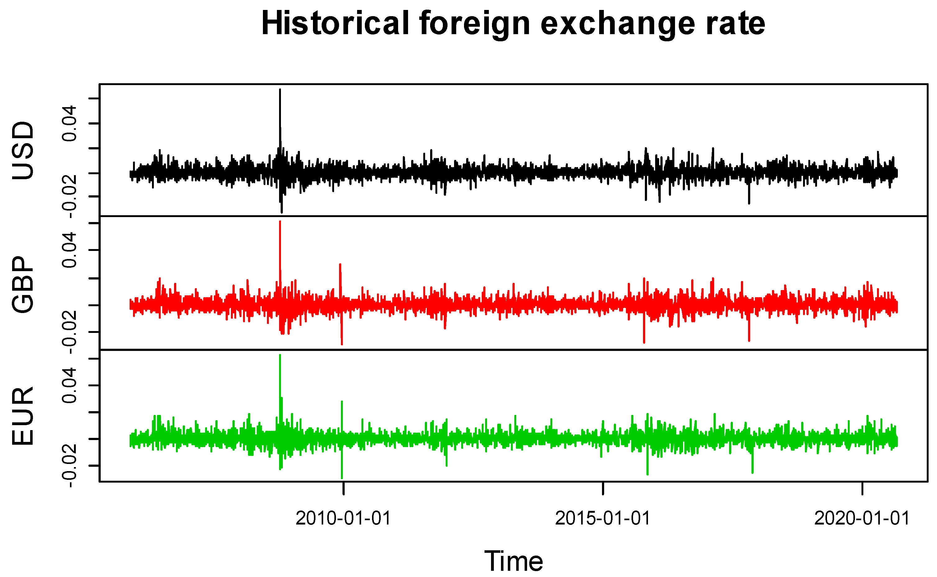
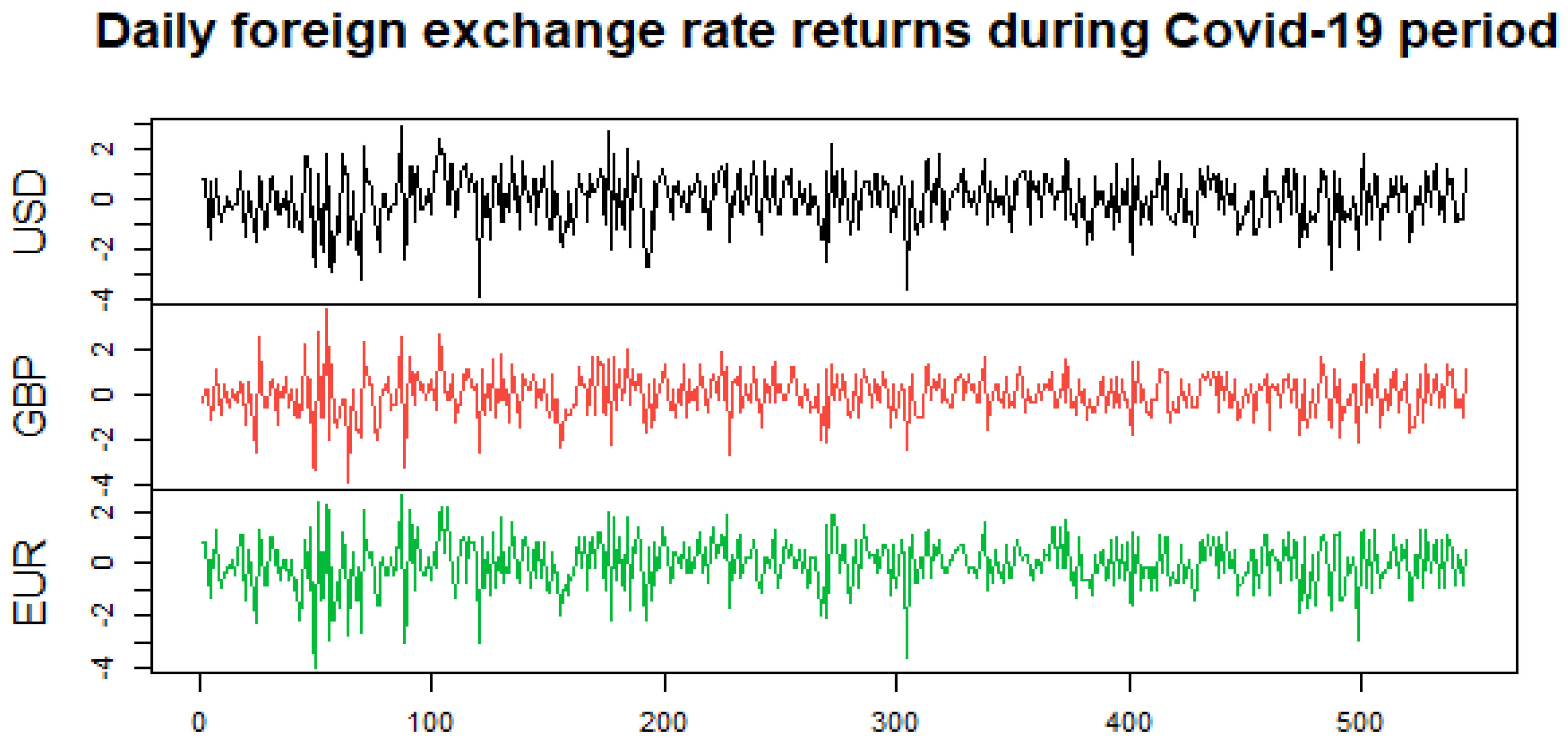
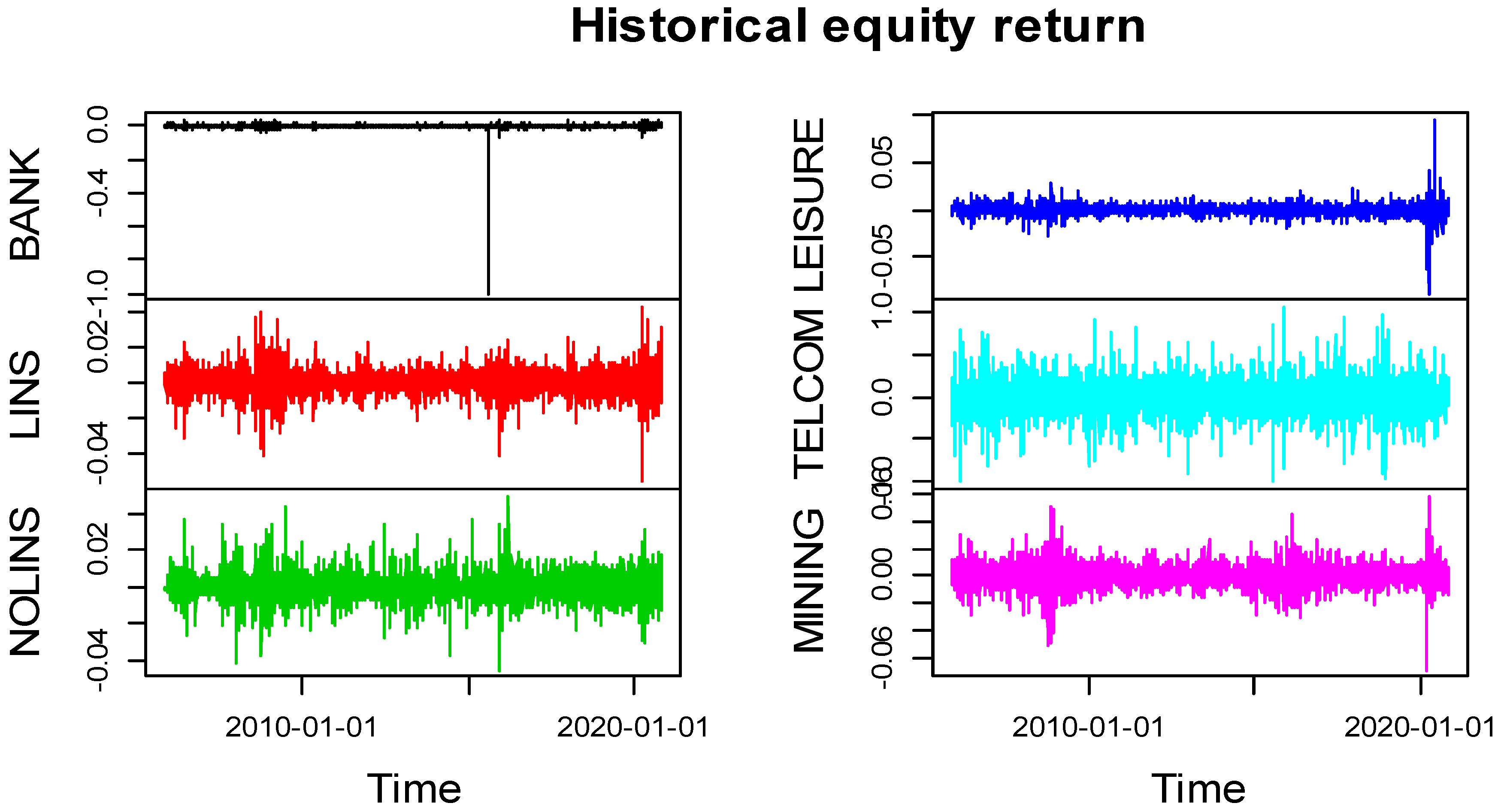
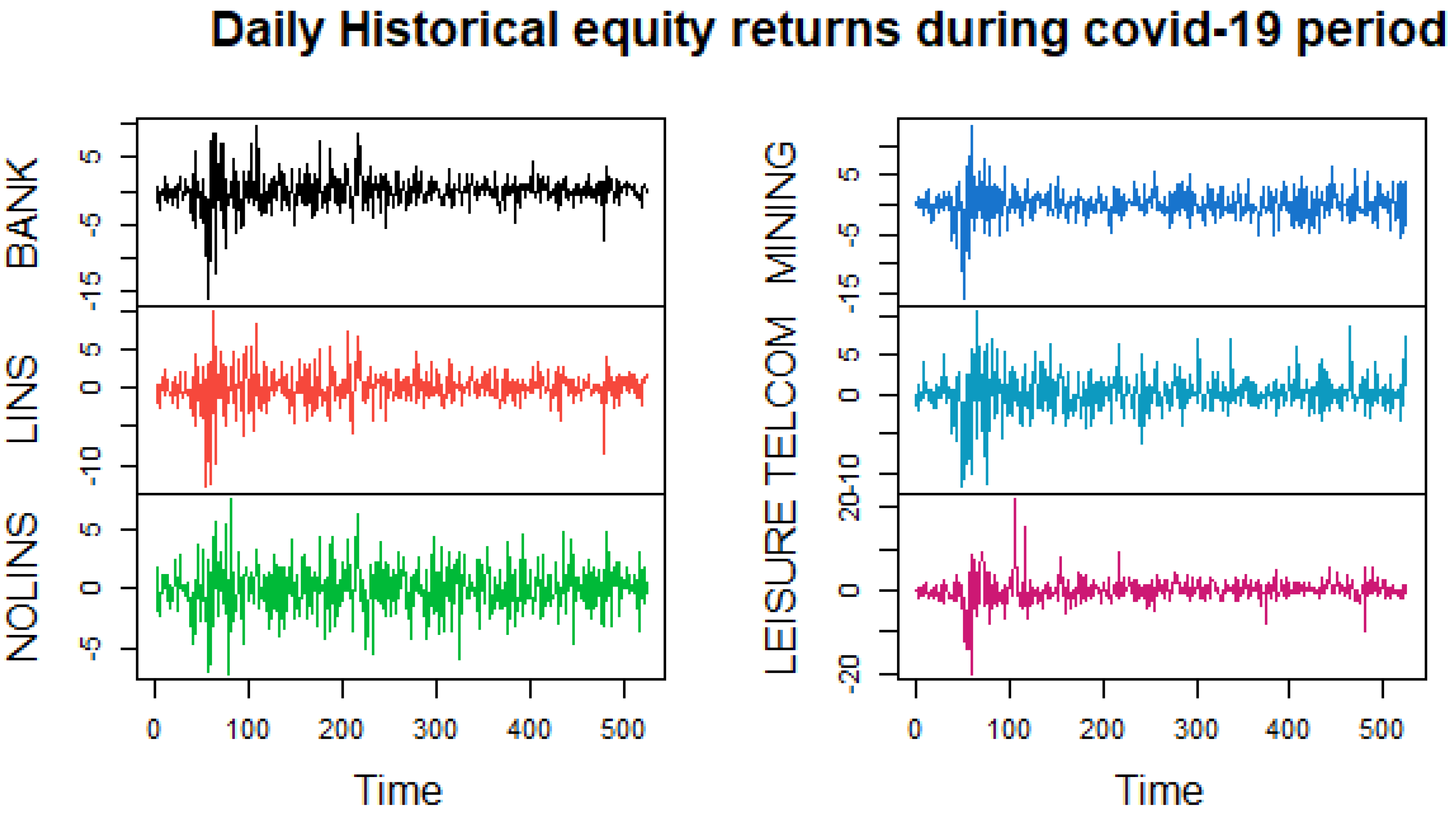
3.1. Sampling and Data Collection

The data for spot and forward exchange rate were obtained from Thomson Reuters Datastream, and those of listed sector were sourced from Inet-BFA Database. This study used the United States dollar’s daily foreign exchange rate (USD), British pound (GBP), and Euro (EUR) against the South African rand. In addition, daily observations of the listed sectors—namely, life insurance, non-life insurance, bank, mining, and leisure and telecommunications that appear in the JSE top 40—were considered in this study. We collected the data in two sets: pre-COVID-19 (3 January 2005 to 31 December 2019) and the COVID-19 period (3 January 2020 to 31 January 2022). The post-COVID-19 data were not available to compare the impact of COVID-19 on the dependence analysis for the stock comprising the JSE indices. The sample was chosen to observe the market behaviour during a normal period and turbulent scenarios such as the recent global financial crisis: the COVID-19 outbreak.

3.2. Marginal Distribution Models

3.2.1. Stochastic Volatility Models

We derived the marginal density of the foreign exchange rate returns using the stochastic volatility (SV) model with t-distributed error to account for the heavy tails and the jump process to account for leverage effect and time variation. The equation for the returns series $\left({\mathrm{Y}}_{\mathrm{t}}\right)$ is as follows:

$${\mathrm{y}}_{\mathrm{t}}={\mathrm{k}}_{\mathrm{y}}{\mathsf{\gamma }}_{\mathrm{t}}+{\left({\mathsf{\lambda }}_{\mathrm{t}}{\mathsf{\epsilon }}_{\mathrm{t}}\right)}^{\frac{1}{2}}\exp \left(\frac{{\mathrm{h}}_{\mathrm{t}}}{2}\right),\mathrm{t}=1,\dots ,\mathrm{T}$$

(1)

$${\mathrm{h}}_{\mathrm{t}+1}=\mathsf{\mu }+\mathsf{\varphi }\left({\mathrm{h}}_{\mathrm{t}}-\mathsf{\mu }\right)+{\mathsf{\sigma }\mathsf{\eta }}_{\mathrm{t}}, \mathrm{t}=0,\dots ,\mathrm{T}-1$$

$${\mathrm{h}}_{\mathrm{t}}\backsim \mathrm{N}(0,{\mathsf{\sigma }}^2/(1-{\mathsf{\theta }}^2))$$

$${\mathsf{\epsilon }}_{\mathrm{t}}\backsim \left(\mathsf{\nu }\right)$$

$${\mathsf{\eta }}_{\mathrm{t}}\backsim \mathrm{N}\left(0,1\right)$$

$${\mathrm{k}}_{\mathrm{t}}\sim \mathrm{N}\left({\mathsf{\mu }}_{\mathrm{s}},{\mathsf{\lambda }}_{\mathrm{s}}\right)$$

where ${\mathrm{h}}_{\mathrm{t}}$ is observed log volatility and ${\mathrm{k}}_{\mathrm{t}}{\mathsf{\gamma }}_{\mathrm{t}}$ is the jump process. $\left(\mathrm{v}\right)$ is a degree of freedom and ${\mathsf{\gamma }}_{\mathrm{t}}$ is a Bernoulli-distributed random variable. We used the stochastic volatility model to filter the financial return to capture the dynamic stylised facts of the volatility of the returns.

3.2.2. GARCH-Type Models

We filtered the residual and captured the remaining distributional stylised facts, such as skewness, leptokurtosis, and heavy tails distribution, using the GJR-GARCH (1,1) models with three distributions, including the normal Gaussian distribution, the skewed Student’s t-distribution, and the semi-parametric volatility model, where the news impact function can be any smooth function. The skewed Student’s t (sstd) innovation best fit the data as it allowed us to capture the leverage effect in the model.

$${\sigma }_t^2={\omega }_0+{\alpha }_1{\epsilon }_{t-1}^2+{\beta }_1{\epsilon }_{t-1}^2+{\gamma }_1{\epsilon }_{t-1}^2{I}_{t-i}$$

(2)

where $I_{t-i}=\{\begin{array}{ccc}1& if& {\epsilon }_{t-i}<0\\ 0& if& {\epsilon }_{t-i}\ge 0\end{array}$. $I_{t-i}$ is a strict white noise process and $I_t~N\left(0,1\right);{\sigma }_{i,t}^2$ is the conditional variance of $Y_{i,t}$ over time, $t$.

3.2.3. Generalised Pareto Distribution (GPD) Function

To correctly specify the extreme value of the residuals from the GJR-GARCH (1,1) models, we used the generalised Pareto distribution (GPD) with a peak over threshold (POT). We applied the limit theorem in selecting the threshold to avoid biased estimates due to the bias–variance tradeoff. Our study used 90% quantile for right tails and 10% quantile for left tails as extreme thresholds. The selected threshold allowed us to model the tails of marginal distributions, where the extreme negative and positive returns fall beyond the extreme thresholds (Koliai 2016). The generalised Pareto distribution function is as follows

$$G_{\psi ,\beta \left(\vartheta \right)}\left(x\right)=\{\begin{array}{ccc}1-(1+\xi {\left(\frac{x}{\beta \left(\vartheta \right)}\right)}^{-1/\psi }& if& \psi \ne 0\\ 1-exp\left(-x/\beta \left(\vartheta \right)\right)& if& \psi =0\end{array}$$

(3)

where $\beta \left(\vartheta \right)>0;x\ge 0 for \xi \ge 0 and 0\le x\le -\frac{\beta \left(\vartheta \right)}{\xi } ;for \xi <0$ and where $\beta$ is the scale and $\psi$ is the shape parameters of the GPD on the lower and upper tails, respectively, or tail index. We chose to use the generalised Pareto distribution (GPD) approximation over the generalised Extreme Value (GEV) because it deals with asymmetries in the tails. We employed the peak over threshold (POT) technique to model the filtered observation from Equation (2) that exceeded a given threshold $\vartheta$. These observations beyond the threshold were considered to constitute the extreme event.

3.3. Dependence Structure Model and Risk Model

We employed the pairwise copula to model the dependence structure between the exchange rate and equity indices return. We used the regular vine copula (R-vine model), the C-vine copula, and D-vine copula to specify the joint-dependent structures and the series’s conditional and unconditional pair dependences. We then selected the most suitable pair copula to model the dependence structure of the foreign exchange rate and equity indices in the JSE market.

3.3.1. Pairwise Copula Approach

Pairwise copula was developed by Bedford and Cooke (2001) and extended by Nikoloulopoulos et al. (2012) and Joe et al. (2010), who applied it to financial data for the first time with two parameters, bivariate-linking the upper tail to a lower tail dependence. It was built using bivariate copulae, where each pair copula could be chosen independently. The methodology’s particularity resides in the fact that asymmetry and tail dependence can be considered when building a more parsimonious model, as in the equation below:

$$f\left(\frac{r}{u}\right)=C_{r,}{u}_j/u_{-j}\left(F\left(\frac{r}{u_{-j}}\right),F\left(\frac{u_j}{u_{-j}}\right)\right).\left(r/u_{-j}\right)$$

(4)

where $C_{r,}{u}_j/u_{-j}$ is the density function of the bivariate copula. The marginal conditional distribution function is given by:

$$F\left(\frac{r}{u}\right)=\frac{\partial C_{r,}{u}_j/u_{-j}\left(F\left(\frac{r}{u_{-j}}\right),F(u_j/u_{-j})\right)}{\partial F\left(\frac{u_j}{u_{-j}}\right)}$$

(5)

From the R-vine copula Function (4), we derived the right (u) and left ($d$) tail dependence as follows:

$$(\begin{array}{c}{\lambda }_u=\begin{array}{cc}lim& P_r\left[X\ge F_X^{-1}\left(x\right)/Y\ge F_Y^{-1}\left(y\right)\right]\\ u\to 1& .\end{array}\\ {\lambda }_d=\begin{array}{cc}lim& P_r\left[X\le F_X^{-1}\left(x\right)/Y\le F_Y^{-1}\left(y\right)\right]\\ u\to 0& .\end{array}\end{array}$$

(6)

This study considered three different pairwise copulae, including D-vine, R-vine (all Gumbel), and C-vine, to model the tail dependence. The downside and upside risks were quantified using the pairwise copula results.

3.3.2. Value at Risk Model

This study employed the VaR-based GJR-GARCH model as it accounts for asymmetry in the conditional variance and the excess kurtosis and skewness. At a given confidence level $\left(1-\alpha \right)$ at time $t$, VaR is given for downside ($d$) and upside (u) as follows:

$$(\begin{array}{c}Va{R}_{\alpha ,t}^d=-{\mu }_t-{\sigma }_t^2{\tau }_{u,v}\left(\alpha \right)\\ Va{R}_{\alpha ,t}^u={\mu }_t+{\sigma }_t^2{\tau }_{u,v}\left(1-\alpha \right)\end{array}$$

(7)

where ${\mu }_t$ and ${\sigma }_t$ represent the conditional mean and conditional variance derived from the stochastic volatility (SV) model.

3.3.3. Backtesting Test

We checked our model’s robustness and validity using the KUPIEC test method of Kupiec (1995), which consists of the unconditional coverage test (UCT) and conditional coverage test (CCT). This test enabled us to assess for the violation of VaR. In this regard, Virdi (2011) argued that the best-fitted VaR model must satisfy both conditional and unconditional coverage tests. On the other hand, Jorion (2007) argued that backtesting helps check whether the actual loss exceeds the estimated VaR. In other words, it is constructed to verify if the actual trading losses align with the forecasted losses. The UCT is based on the likelihood ratio test statistic as follows:

$$L{R}_{POF}=-2Log\left[\frac{{(1-pr)}^{T-x}p{r}^x}{{(1-\frac{x}{T})}^{T-x}{(\frac{x}{T})}^x}\right]$$

(8)

where $x$ represents the number of exceptions, $Pr$ is the probability of an exception for a given confidence level, and $T$ is the number of trials. In this case, the number of trials is 250 trading days in a year.

4. Results and Discussion

Table 1. Parameter estimates for marginal models using GJR-GARCH (1,1).

		Shape	${\mathit{a}}_1$	$\mathit{\omega }$	${\mathit{\alpha }}_1$	${\mathit{\beta }}_1$	${\mathit{\gamma }}_1$	AIC	Log-Lik	BIC
Exchange rate	USD/ZAR	1.271 (0.073) ***	−0.046 (0.013) ***	0.000 (0.000)	0.055 (0.010) ***	0.953 (0.008) ***	−0.044 (0.009) ***	−8.151	17,111.3	−8.142
	GBP/ZAR	1.200 (0.031) ***	−0.035 (0.013) **	0.000 (0.000)	0.066 (0.002) ***	0.935 (0.005) ***	−0.041 (0.011) ***	−8.259	17,338.3	−8.250
	EUR/ZAR	1.152 (0.048) ***	−0.021 (0.013)	0.000 (0.000)	0.078 (0.024	0.923 (0.020) ***	−0.066 (0.017) ***	−8.329	17,485.8	−8.320
Equity index	BANK	2.902 (0.425) ***	0.735 (0.027) ***	0.024 (0.022)	0.000 (0.087)	0.726 (0.257) **	0.483 (0.133) ***	0.849	−1491.2	0.860
	LINS	2.811 (0.197) ***	0.739 (0.015) ***	0.025 (0.006) ***	0.000 (0.032)	0.706 (0.071) ***	0.553 (0.082) ***	0.844	−1481.8	0.854
	NOLINS	2.828 (0.171) ***	0.727 (0.013) ***	0.066 (0.007) ***	0.000 (0.025)	0.380 (0.066) ***	0.704 (0.090) ***	0.833	−1462.2	0.843
	LEISURE	2.707 (0.207) ***	0.732 (0.014) ***	0.052 (0.026) *	0.000 (0.054)	0.495 (0.253) ***	0.630 (0.051) ***	0.840	−1475.6	0.851
	TELCOM	3.559 (0.330) ***	0.710 (0.024) ***	0.068 (0.009) ***	0.000 (0.052)	0.470 (0.084) ***	0.441 (0.091) ***	0.925	−1624.7	0.935
	MINING	2.998 (0.054) ***	0.744 (0.010) ***	0.015 (0.006) *	0.000 (0.028)	0.811 (0.084) ***	0.348 (0.054) ***	0.852	−1497.0	0.863

Notes: This table reports the estimated coefficients of the conditional mean and conditional variance for GJR-GARCH (1,1) under Student’s t-distribution. The robust standard error is in brackets, and the asterisks represent the significance of the p-values. *** Indicates significance at 1% level, ** indicates significance level at 5% level, * indicates significance at 10% level; in parentheses is the standard error. LINS is life insurance, NOLINS is non-life insurance, and TELCOM is telecommunications. Log-lik is log-likelihood.

displays the estimated parameters of the GJR-GARCH (1,1) model with different distributions.

The parameter beta is primarily positive and significant at a 1% confidence level. The significance and positive value of the beta parameters imply that the stock and foreign exchange markets’ volatility in the previous period is positively transmitted into the volatility of the current periods under market conditions. Thus, the parameter beta represents the leverage. The shape parameter of the model is statistically significant and positive for all markets, indicating the presence of fat tails. We observe positive leverage in the equity market, implying that negative return shock causes greater volatility.

In contrast, the foreign exchange market exhibits negative leverage, suggesting that high negative returns are followed by higher volatility growth. We may conclude that the foreign exchange market is mature with persistent volatility clustering. Thus, bad news in these markets has a severe implication for the volatility of this market during extreme events.

Table 2. Parameter estimates for marginal models using SV model with heavy tail innovations and AR(1) structure.

Parameter	Mean	SD	95% Interval	Inefficiency	Parameter	Mean	SD	95% Interval	Inefficiency
Forex market—USD/ZAR					Equity market—BANK
$\mu$	−11.16	0.155	−10.91	2295	$\mu$	−10.152	0.162	−9.890	5326
$\sigma$	0.983	0.013	0.993	307	$\sigma$	0.133	0.016	0.161	121
$\phi$	0.987	0.004	0.121	142	$\phi$	0.984	0.004	0.991	213
$\eta$	9.612	1.981	13.25	66	$\eta$	9.319	1.140	11.328	177
$\upsilon$	0.003	0.000	0.004	2295	$\upsilon$	0.006	0.000	0.007	5326
$\gamma$	0.009	0.002	0.014	142	$\gamma$	0.018	0.004	0.026	121
Forex market—GBP/ZAR					Equity market—LIFE INSURANCE (LINS)
$\mu$	−11.30	0.117	−11.19	1037	$\mu$	−10.341	0.16	−10.074	2880
$\sigma$	0.125	0.022	0.165	83	$\sigma$	0.156	0.001	0.184	135
$\phi$	0.978	0.007	0.989	106	$\phi$	0.982	0.000	0.990	281
$\eta$	6.881	0.979	8.821	120	$\eta$	27.505	1.000	44.771	22
$\upsilon$	0.003	0.002	0.003	1037	$\upsilon$	0.005	0.000	0.006	2880
$\gamma$	0.016	0.005	0.027	83	$\gamma$	0.024	0.000	0.034	135
Forex market—EUR/ZAR					Equity market—NON-LIFE INSURANCE (NOLINS)
$\mu$	−11.47	0.107	−11.30	1200	$\mu$	−10.413	0.088	−10.27	264
$\sigma$	0.135	0.024	0.176	76	$\sigma$	0.309	0.060	0.958	54
$\phi$	0.975	0.008	0.986	108	$\phi$	0.987	0.004	0.993	307
$\eta$	6.282	0.816	7.742	115	$\eta$	10.670	5.633	18.740	20
$\upsilon$	0.003	0.000	0.003	1200	$\upsilon$	0.005	0.000	0.006	264
$\gamma$	0.018	0.007	0.031	76	$\gamma$	0.099	0.039	0.180	42
Equity market—LEISURE					Equity market—TELCOM
$\mu$	−10.94	0.153	−10.695	1508	$\mu$	−3.65	0.040	−3.58	1240
$\sigma$	0.168	0.029	0.218	46	$\sigma$	0.44	0.045	0.52	156
$\phi$	0.978	0.007	0.989	71	$\phi$	0.72	0.045	0.79	151
$\eta$	13.222	6.292	25.178	13	$\eta$	39.78	8.151	49.27	41
$\upsilon$	0.004	0.000	0.004	1508	$\upsilon$	0.16	0.003	0.17	1240
$\gamma$	0.029	0.010	0.047	46	$\gamma$	0.20	0.040	0.27	156
Equity market—MINING
$\mu$	−9.913	0.222	−9.571	5461
$\sigma$	0.099	0.010	0.116	211
$\phi$	0.991	0.002	0.995	622
$\eta$	34.847	8.482	48.373	46
$\upsilon$	0.007	0.000	0.008	5461
$\gamma$	0.010	0.002	0.013	211

Note: This table presents the parameter estimates output for 10,000 replications from the AR(1)-SV model. It presents the mean and standard deviation of the posterior estimates across 10,000 samples. The upper tail is 95th percentile, and inefficiency denotes the inefficiency factors.

displays the Markov Chain Monte Carlo (MCMC) estimation result of the SV model with heavy tail innovation in the Autoregressive (AR) framework. We report the posterior mean and standard deviation for each parameter. We observe that foreign exchange rate and equity markets indicate that there is a high persistence of volatility with heavy tail distribution close to 0.98, except for the telecommunications index. The inefficiency factor indicates leverage effects. The result shows that our model built on the AR-SV model is designed to capture not only the higher-order volatility but also the heavy tail and leverage effects.

We construct pairwise copulae to analyse the dependence structure between the daily exchange rates and equity indices series. Three vine copulae, namely, R-vine, C-vine, and D-vine, were employed, and the results are reported in

Table A1. Parameter estimates of the dependence structures using R-vine model.

Tree	Serie 1	Serie 2	Conditioning Series	Pair-Copula	1st Par	2nd Par	Tau	Utd	ltd
Panel 1: equity market
1	LINS	NOLINS		BB1	0.27	1.08	0.19	0.11	0.10
	LINS	LEISURE		Student’s t	0.38	5.25	0.25	0.14	0.14
	BANK	TELCOM		BB1_270	−0.07	−1.00	−0.03	-	-
	LINS	BANK		Student’s t	0.70	4.90	0.49	0.35	0.35
	MINING	LINS		Student’s t	0.43	3.97	0.29	0.22	0.22
2	LEISURE	NOLINS	LINS	Student’s t	0.14	13.19	0.09	0.01	0.01
	BANK	LEISURE	LINS	Student’s t	0.17	10.99	0.11	0.01	0.01
	LINS	TELCOM	BANK	S-BB1	0.00	1.00	0.00	0.00	0.00
	MINING	BANK	LINS	Student’s t	0.10	5.88	0.06	0.05	0.05
3	BANK	NOLINS	LEISURE, LINS	Student’s t	0.09	25.61	0.06	0.00	0.00
	MINING	LEISURE	BANK, LINS	Student’s t	0.03	9.68	0.02	0.01	0.01
	MINING	TELECOM	LINS, BANK	BB1_90	−0.00	−1.01	−0.01	-	-
4	MINING	NOLINS	BANK, LEISURE, LINS	Student’s t	−0.01	20.62	−0.01	0.00	0.00
	TELCOM	LEISURE	MINING, BANK, LINS	BB1_270	−0.01	−1.00	−0.00	-	-
5	TELCOM	NOLINS	MINING, BANK, LEISURE, LINS	S-BB1	0.05	1.00	0.03	0.00	0.01
Panel 2: foreign exchange market
1	USD/ZAR	GBP/ZAR		Student’s t	0.17	4.13	0.11	0.11	0.11
	EUR/ZAR	USD/ZAR		Student’s t	−0.02	9.22	−0.01	0.11	0.11
2	EUR/ZAR	GBP/ZAR	USD/ZAR	Student’s t	0.01	14.45	0.00	0.00	0.00
Panel 3: mixture market
1	LINS	NOLINS		S-BB1	0.97	1.08	0.38	0.52	0.10
	LINS	LEISURE		S-BB1	1.05	1.14	0.42	0.56	0.16
	LINS	MINING		S-BB1	1.22	1.16	0.46	0.61	0.18
	BANK	LINS		S-BB1	1.60	1.45	0.62	0.74	0.39
	TELCOM	BANK		Frank	0.26	0.00	0.03	-	-
	USD/ZAR	GBP		Joe	1.84	0.00	0.32	0.54	-
	TELCOM	USD/ZAR		Joe	1.56	0.00	0.24	0.44	-
	EUR/ZAR	TELCOM		Joe	1.54	0.00	0.23	0.43	-
2	LEISURE	NOLINS	LINS	BB1	0.02	1.16	0.15	0.19	0.00
	BANK	LEISURE	LINS	BB1	0.07	1.12	0.14	0.14	0.00
	BANK	MINING	LINS	Student’s t	0.13	6.91	0.08	0.04	0.04
	TELCOM	LINS	BANK	Joe	1.05	0.00	0.03	0.07	-
	EUR/ZAR	BANK	TELCOM	S-BB1	0.32	1.01	0.15	0.12	0.02
	TELCOM	GBP/ZAR	BANK	Joe	1.17	0.00	0.09	0.19	-
	EUR/ZAR	USD/ZAR	TELCOM	Joe	1.23	0.00	0.12	0.25	-
3	BANK	NOLINS	LEISURE, LINS	BB1	0.06	1.05	0.08	0.07	0.00
	MINING	LEISURE	BANK, BANK	Student’s t	0.07	10.14	0.04	0.01	0.01
	TELCOM	MINING	BANK, LINS	Frank	0.02	0.00	0.00	-	-
	EUR/ZAR	LINS	TELCOM, BANK	Student’s t	0.02	14.15	0.01	0.00	0.00
	GBP/ZAR	BANK	EUR/ZAR, TELCOM	Joe	1.19	0.00	0.10	0.21	-
	EUR/ZAR	GBP/ZAR	TELCOM, USD/ZAR	Joe	1.13	0.00	0.07	0.16	-
4	MINING	NOLINS	BANK, LEISURE, LINS	Joe	1.05	0.00	0.03	0.07	-
	TELCOM	LEISURE	MINING, BANK, LINS	Joe	1.11	0.00	0.06	0.13	-
	EUR/ZAR	MINING	TELCOM, BANK, LINS	Student’s t	0.01	12.06	0.01	0.00	0.00
	GBP/ZAR	LINS	EUR/ZAR, TELCOM, BANK	S-Joe	1.19	0.00	0.07	0.16	-
	GBP/ZAR	BANK	USD/ZAR, EUR/ZAR, TELCOM	BB1	0.00	1.08	0.07	0.09	0.00
5	TELCOM	NOLINS	MINING, BANK, LEISURE, LINS	Joe	1.16	0.00	0.08	0.18	-
	EUR/ZAR	LEISURE	TELCOM, MINING, BANK, LINS	Joe	1.05	0.00	0.03	0.06	-
	USD/ZAR	LEISURE	EUR/ZAR, TELCOM, BANK, LINS	Joe	1.03	0.00	0.02	0.04	-
	GBP/ZAR	LINS	USD/ZAR, EUR/ZAR, LEISURE, LINS	Student’s t	0.01	13.59	0.00	0.00	0.00
6	EUR/ZAR	NOLINS	TELCOM, MINING, BANK, LEISURE, LINS	Gumbel	1.03	0.00	0.03	0.04	-
	USD/ZAR	LEISURE	EUR/ZAR, TELCOM, MINING, BANK, LINS	Student’s t	0.01	15.00	0.01	0.00	0.00
	GBP/ZAR	MINING	USD/ZAR, EUR/ZAR, LEISURE, BANK, LINS	S-Joe	1.01	0.00	0.01	-	0.02
7	USD/ZAR	NOLINS	EUR/ZAR, TELCOM, MINING, BANK, LEISURE, LINS	Joe	1.03	0.00	0.02	0.04	-
	GBP/ZAR	LEISURE	USD/ZAR, EUR/ZAR, LEISURE, MINING, BANK, LINS	Joe	1.05	0.00	0.03	0.06	-
8	GBP/ZAR	NOLINS	USD/ZAR, EUR/ZAR, TELCOM, MINING, BANK, LEISURE, LINS	Joe	1.02	0.00	0.01	0.02	-

Note: Table A1 exhibits the dependence structure analysis using the R-vine copula. Several bivariate copulae are used: BB1 denotes Clayton–Gumbel, BB1_270 denotes the rotated Clayton–Gumbel, S-BB1 represents the survival of Clayton–Gumbel. We observed the dependence between two assets conditioning to one or more other assets.

,

Table A2. Parameter estimates of the dependence structures using C-vine model.

Tree	Serie 1	Serie 2	Conditioning Series	Pair-Copula	1st Par	2nd Par	Tau	Utd	ltd
Panel 1: equity indices
1	LINS	LEISURE		S-Gumbel	1.32	0.00	0.24	-	0.31
	LINS	TELCOM		C_270	−0.06	0.00	−0.03	-	-
	LINS	NOLINS		S-Gumbel	1.22	0.00	0.18	-	0.24
	LINS	BANK		S-Gumbel	1.93	0.00	0.48	-	0.57
	MINING	LINS		S-Gumbel	1.39	0.00	0.28	-	0.36
2	BANK	LEISURE	LINS	Gumbel	1.13	0.00	0.11	0.15	-
	BANK	TELCOM	LINS	C_270	−0.02	0.00	−0.01	-	-
	BANK	NOLINS	LINS	Frank	0.71	0.00	0.08	-	-
	MINING	BANK	BANK, LINS	Gumbel	1.09	0.00	0.08	0.11	-
3	NOLINS	LEISURE	BANK, LINS	S-Gumbel	1.07	0.00	0.06	-	0.09
	NOLINS	TELCOM	BANK, LINS	S-Clayton	0.05	0.00	0.03	0.00	-
	MINING	NOLINS	BANK, LINS	C_90	−0.02	0.00	−0.01	-	-
4	MINING	LEISURE	NOLINS, BANK, LINS	S-Gumbel	1.03	0.00	0.03	-	0.04
	MINING	TELCOM	NOLINS, BANK, LINS	C_270	−0.01	0.00	−0.00	-	-
5	TELCOM	LEISURE	MINING, NOLINS, BANK, LINS	C_270	−0.00	0.00	−0.00	-	-
Panel 2: exchange rates
1	USD/ZAR	GBP/ZAR		Gumbel	1.13	0.00	0.12	0.15	-
	EUR/ZAR	USD/ZAR		G_90	−1.03	0.00	−0.02	-	-
2	EUR/ZAR	GBP/ZAR	USD/ZAR	S-Gumbel	1.02	0.00	0.02	-	0.03
Panel 3: mixed system
1	LINS	MINING		S_Gumbel	1.49	0.00	0.33	-	0.41
	LINS	NOLINS		S-Gumbel	1.30	0.00	0.23	-	0.29
	LINS	USD/ZAR		S_Clayton	0.60	0.00	0.23	0.32	-
	LINS	TELCOM		Frank	0.34	0.00	0.04	-	-
	LINS	LEISURE		S-Gumbel	1.14	0.00	0.29	-	0.37
	LINS	GBP/ZAR		S-Clayton	0.59	0.00	0.23	0.31	-
	LINS	BANK		S-Gumbel	2.11	0.00	0.52	-	0.61
	EUR/ZAR	LINS		S-Clayton	0.60	0.00	0.23	0.31	-
2	BANK	MINING	LINS	Gumbel	1.20	0.00	0.17	0.22	-
	BANK	NOLINS	LINS	Gumbel	1.20	0.00	0.17	0.22	-
	BANK	USD/ZAR	LINS	S-Clayton	0.19	0.00	0.09	0.03	-
	BANK	TELCOM	LINS	Frank	0.08	0.00	0.01	-	-
	BANK	LEISURE	LINS	Gumbel	1.25	0.00	0.20	0.26	-
	BANK	GBP/ZAR	LINS	S-Gumbel	0.24	0.00	0.11	0.05	-
	EUR/ZAR	BANK	LINS	S-Clayton	0.24	0.00	0.11	0.06
3	GBP/ZAR	MINING	BANK, LINS	Gumbel	1.07	0.00	0.06	0.09	-
	GBP/ZAR	NOLINS	BANK, LINS	S-Clayton	0.19	0.00	0.09	0.02	-
	GBP/ZAR	USD/ZAR	BANK, LINS	Gumbel	1.28	0.00	0.22	0.28	-
	GBP/ZAR	TELCOM	BANK, LINS	S-Clayton	0.25	0.00	0.09	0.03	-
	GBP/ZAR	LEISURE	BANK, LINS	S-Clayton	0.20	0.00	0.09	0.03	-
	EUR/ZAR	GBP/ZAR	BANK, LINS	Gumbel	1.13	0.00	0.11	0.15	-
4	LEISURE	MINING	GBP/ZAR, BANK, LINS	Gumbel	1.12	0.00	0.10	0.14	-
	LEISURE	NOLINS	GBP/ZAR, BANK, LINS	S-Clayton	0.48	0.00	0.19	0.23	-
	LEISURE	USD/ZAR	GBP/ZAR, BANK, LINS	Gumbel	1.06	0.00	0.06	0.08
	LEISURE	TELCOM	GBP/ZAR, BANK, LINS	S-Gumbel	0.31	0.00	0.13	0.11	-
	EUR/ZAR	LEISURE	GBP/ZAR, BANK, LINS	Gumbel	1.05	0.00	0.05	0.07	-
5	TELCOM	MINING	LEISURE, GBP/ZAR, BANK, LINS	S-Gumbel	0.19	0.00	0.05	0.07	-
	TELCOM	NOLINS	LEISURE, GBP/ZAR, BANK,LINS	S-Gumbel	0.26	0.00	0.11	0.07	-
	TELCOM	USD/ZAR	LEISURE, GBP/ZAR, BANK,LINS	Gumbel	1.08	0.00	0.08	0.10	-
	EUR/ZAR	TELCOM	LEISURE, GBP/ZAR, BANK,LINS	S-Gumbel	0.21	0.00	0.04	0.05	-
6	EUR/ZAR	MINING	TELCOM, LEISURE, GBP/ZAR, BANK, LINS	Gumbel	1.04	0.00	0.04	0.05	-
	EUR/ZAR	NOLINS	TELCOM, LEISURE, GBP/ZAR, BANK, LINS	Gumbel	1.04	0.00	0.04	0.06	-
	EUR/ZAR	USD/ZAR	TELCOM, LEISURE, GBP/ZAR, BANK, LINS	Gumbel	1.06	0.00	0.04	0.07	-
7	NOLINS	MINING	EUR/ZAR,TELCOM, LEISURE,GBP/ZAR,BANK, LINS	Gumbel	1.04	0.00	0.04	0.06	-
	USD/ZAR	NOLINS	EUR/ZAR, TELCOM, LEISURE,GBP/ZAR,BANK, LINS	Gumbel	1.03	0.00	0.03	0.04	-
8	GBP/ZAR	MINING	NOLINS, EUR/ZAR, TELCOM, LEISURE,GBP/ZAR,BANK, LINS	Gumbel	1.04	0.00	0.04	0.05	-

Note: Table A2 exhibits the dependence structure analysis using the C-vine copula. Several bivariate copulae families are used: S-Clayton denotes Survival—Clayton; S-Gumbel denote Survival—Gumbel; S-BB1 represents the survival of Clayton–Gumbel. We observed the dependence between two assets conditioning to one or more other assets.

and

Table A3. Parameter estimates of the dependence structures using D-vine model.

Tree	Serie 1	Serie 2	Conditioning Series	Pair-Copula	1st Par	2nd Par	Tau	Utd	ltd
Panel 1: equity indices
1	LINS	LEISURE		S-Gumbel	1.32	0.00	0.24	-	0.31
	LINS	TELCOM		C_270	−0.06	0.00	−0.03	-	-
	LINS	NOLINS		S-Gumbel	1.22	0.00	0.18	-	0.24
	LINS	BANK		S-Gumbel	1.93	0.00	0.48	-	0.57
	MINING	LINS		S-Gumbel	1.39	0.00	0.28	-	0.36
2	BANK	LEISURE	LINS	Gumbel	1.13	0.00	0.11	0.15
	BANK	TELCOM	LINS	C_270	−0.02	0.00	−0.01	-	-
	BANK	NOLINS	LINS	Frank	0.71	0.00	0.08	-	-
	MINING	BANK	BANK, LINS	Gumbel	1.09	0.00	0.08	0.11	-
3	NOLINS	LEISURE	BANK, LINS	S-Gumbel	1.07	0.00	0.06	-	0.09
	NOLINS	TELCOM	BANK, LINS	S-Clayton	0.05	0.00	0.03	0.00	-
	MINING	NOLINS	BANK, LINS	C_90	−0.02	0.00	−0.01	-	-
4	MINING	LEISURE	NOLINS, BANK, LINS	S-Gumbel	1.03	0.00	0.03	-	0.04
	MINING	TELCOM	NOLINS, BANK, LINS	C_270	−0.01	0.00	−0.00	-	-
5	TELCOM	LEISURE	MINING, NOLINS, BANK, LINS	C_270	−0.00	0.00	−0.00	-	-
Panel 2: exchange rates
1	USD/ZAR	GBP/ZAR		Gumbel	1.13	0.00	0.12	0.15	-
	EUR/ZAR	USD/ZAR		G_90	−1.03	0.00	−0.02	-	-
2	EUR/ZAR	GBP/ZAR	USD/ZAR	S-Gumbel	1.02	0.00	0.02	-	0.03
Panel 3: mixed system
1	LINS	MINING		S_Gumbel	1.49	0.00	0.33	-	0.41
	LINS	NOLINS		S-Gumbel	1.30	0.00	0.23	-	0.29
	LINS	USD/ZAR		S_Clayton	0.60	0.00	0.23	0.32	-
	LINS	TELCOM		Frank	0.34	0.00	0.04	-	-
	LINS	LEISURE		S-Gumbel	1.14	0.00	0.29	-	0.37
	LINS	GBP/ZAR		S-Clayton	0.59	0.00	0.23	0.31	-
	LINS	BANK		S-Gumbel	2.11	0.00	0.52	-	0.61
	EUR/ZAR	LINS		S-Clayton	0.60	0.00	0.23	0.31	-
2	BANK	MINING	LINS	Gumbel	1.20	0.00	0.17	0.22	-
	BANK	NOLINS	LINS	Gumbel	1.20	0.00	0.17	0.22	-
	BANK	USD/ZAR	LINS	S-Clayton	0.19	0.00	0.09	0.03	-
	BANK	TELCOM	LINS	Frank	0.08	0.00	0.01	-	-
	BANK	LEISURE	LINS	Gumbel	1.25	0.00	0.20	0.26	-
	BANK	GBP/ZAR	LINS	S-Gumbel	0.24	0.00	0.11	0.05	-
	EUR/ZAR	BANK	LINS	S-Clayton	0.24	0.00	0.11	0.06
3	GBP/ZAR	MINING	BANK, LINS	Gumbel	1.07	0.00	0.06	0.09	-
	GBP/ZAR	NOLINS	BANK, LINS	S-Clayton	0.19	0.00	0.09	0.02	-
	GBP/ZAR	USD/ZAR	BANK, LINS	Gumbel	1.28	0.00	0.22	0.28	-
	GBP/ZAR	TELCOM	BANK, LINS	S-Clayton	0.25	0.00	0.09	0.03	-
	GBP/ZAR	LEISURE	BANK, LINS	S-Clayton	0.20	0.00	0.09	0.03	-
	EUR/ZAR	GBP/ZAR	BANK, LINS	Gumbel	1.13	0.00	0.11	0.15	-
4	LEISURE	MINING	GBP/ZAR, BANK, LINS	Gumbel	1.12	0.00	0.10	0.14	-
	LEISURE	NOLINS	GBP/ZAR, BANK, LINS	S-Clayton	0.48	0.00	0.19	0.23	-
	LEISURE	USD/ZAR	GBP/ZAR, BANK, LINS	Gumbel	1.06	0.00	0.06	0.08
	LEISURE	TELCOM	GBP/ZAR, BANK, LINS	S-Gumbel	0.31	0.00	0.13	0.11	-
	EUR/ZAR	LEISURE	GBP/ZAR, BANK, LINS	Gumbel	1.05	0.00	0.05	0.07	-
5	TELCOM	MINING	LEISURE, GBP/ZAR, BANK, LINS	S-Gumbel	0.19	0.00	0.05	0.07	-
	TELCOM	NOLINS	LEISURE, GBP/ZAR, BANK,LINS	S-Gumbel	0.26	0.00	0.11	0.07	-
	TELCOM	USD/ZAR	LEISURE, GBP/ZAR, BANK,LINS	Gumbel	1.08	0.00	0.08	0.10	-
	EUR/ZAR	TELCOM	LEISURE, GBP/ZAR, BANK, LINS	S-Gumbel	0.21	0.00	0.04	0.05	-
6	EUR/ZAR	MINING	TELCOM, LEISURE, GBP/ZAR, BANK, LINS	Gumbel	1.04	0.00	0.04	0.05	-
	EUR/ZAR	NOLINS	TELCOM, LEISURE, GBP/ZAR, BANK, LINS	Gumbel	1.04	0.00	0.04	0.06	-
	EUR/ZAR	USD/ZAR	TELCOM, LEISURE, GBP/ZAR, BANK, LINS	Gumbel	1.06	0.00	0.04	0.07	-
7	NOLINS	MINING	EUR/ZAR, TELCOM, LEISURE, GBP/ZAR, BANK, LINS	Gumbel	1.04	0.00	0.04	0.06	-
	USD/ZAR	NOLINS	EUR/ZAR, TELCOM, LEISURE, GBP/ZAR, BANK, LINS	Gumbel	1.03	0.00	0.03	0.04	-
8	GBP/ZAR	MINING	NOLINS, EUR/ZAR, TELCOM, LEISURE, GBP/ZAR, BANK, LINS	Gumbel	1.04	0.00	0.04	0.05	-

Note: Table A3 exhibits the dependence structure analysis using the D-vine copula. Several bivariate copulae families are used: S-Clayton denote Survival—Clayton; S-Gumbel denotes Survival—Gumbel; S-BB1 represents the survival of Clayton–Gumbel. We observed the dependence between two assets conditioning to one or more other assets.

(see Appendix A). We focus on lower and upper tail dependence and find that each bivariate copula has a more substantial upper tail dependence in the mixture market. However, the foreign exchange and equity markets have both upper and lower tail dependence. The results indicate that the R-vine copula best models the dependence structure of these series compared to C-vine and D-vine copulae. In addition, we find that equity index and foreign exchange rate market exhibit an asymmetric dependence structure. Hence, the JSE index has a greater VaR exposure to foreign exchange rate volatility.

Table 3. Model assessment based on Vuong test for non-nested models.

Panel A: Before COVID-19 (January 2005 to December 2019)
Markets	Model	Log-Lik	AIC	BIC	Clarke Test			Vuong Test
					Wo/cor	AIC	BIC	Wo/cor	AIC	BIC
Equity indices	R-vine	2454.12	−4848.23	−4663.2	1816	1816	1816	3.87 ***	3.87 ***	3.87 ***
	C-vine	2256.61	−4483.23	−4390.71	1455 ***	1483 ***	1590 ***	−6.15 ***	−5.56 ***	−3.73 ***
	D-vine	2451.09	−4556.18	−4714.32	1810	1803	1778	3.81 ***	3.96 ***	4.40 ***
Exchange rates	R-vine	150.88	−289.77	−252.76	2044	2044	2044	4.25 ***	4.25 ***	4.25 ***
	C-vine	87.79	−169.57	−151.07	1574 ***	1600 ***	1672 ***	−1.12	−0.98	−0.56
	D-vine	150.88	−288.77	−252.76	2038	2030	2005 ***	4.30 ***	4.14 ***	3.66 ***
Mixed System	R-vine	3605.23	−7108.46	−6786.83	1500	1555 *	1723 ***	−1.77 *	−0.25	4.31 ***
	C-vine	2997.24	−5922.49	−5695.46	927 ***	939 ***	970 ***	−20.07 ***	−19.69 ***	−18.55 ***
	D-vine	3493.24	−6896.49	−6612.69	927 ***	939 ***	970 ***	−4.22 ***	−4.04 ***	−3.51 ***
Panel B: COVID-19 Period (January 2020 to January 2022)
Equity indices	R-vine	591.96	−1123.92	−996.07	246	234 *	208 ***	−0.645	−1.907	−4.596 ***
	C-vine	595.79	−1131.59	−1003.74	240	229	205 ***	−0.610	−1.642	−3.842 ***
	D-vine	594.31	−1140.61	−1038.34	270	257	231 ***	−0.338	−1.291	−3.321 ***
Exchange rates	R-vine	722.09	−1432.18	−1406.38	327	327 ***	327 ***	2.506	2.506 *	2.506 *
	C-vine	704.61	−1397.23	−1371.42	327	327 ***	327 ***	2.506	2.506 *	2.506 *
	D-vine	599.93	−1153.86	−1055.85	327	327 ***	327 ***	2.506	2.506 *	2.506 *
Mixed System	R-vine	1341	−2538.01	−2228.35	262	237 *	208 ***	1.630	−0.279	−4.348 ***
	C-vine	1340.46	−2568.92	−2328.08	274	262	246	1.882	1.351	0.220
	D-vine	1333.28	−2522.56	−2212.9	274	262	246	1.518	−0.143	−3.684 ***

Note: This table reports the likelihood ratio test (LR) for model selection and non-nested hypothesis to check model specifications and selection. We test whether the competing model is correctly specified and whether the model is nested, non-nested, or overlapping. According to Vuong (1989), the non-nested hypothesis test should be interpreted as a “model-specification test”; the likelihood ratio (log-lik) is reported in column 3. The initial model is C-vine copula, and the competing models are the R- and D-vine copulae. The asterisks *** indicates significance at 1% level, and * indicates significance at 10% level.

displays the AIC for the three vine copula models before and during the COVID-19 pandemic periods. The results show that overall, the R-vine copula is superior for the three sets of the portfolio (foreign exchange, equity indices, and mixed portfolio) during the period of normal market activities. The C-vine risk-based specification outperforms the alternative R- and D-vine copulae during the COVID-19 pandemic. This result contradicts Zhang et al. (2014), who argue that the D-vine copula model is superior to other vine copulae. However, their analysis was conducted using a portfolio of stock indices.

We assessed our model using the Vuong (1989) and Clarke (2007) test to select the best-fitted vine copula for value-at-risk estimation. The test statistic result of model assessment for non-nested models is reported in Table 3. Under a null hypothesis that the C-vine model fits the data-generating process, we tested for a non-nested model. We considered the C-vine baseline model and compared the R and D vine models against the baseline model. A value with an asterisk indicates rejection of the null hypothesis. The Vuong test showed that R-vine is statistically significant for all of the markets. The Clarke test does not satisfy the null hypothesis in the equity markets or exchange rate market, although the condition is significant for the hybrid system. The Vuong and Clarke test used as a goodness-of-fit procedure shows that the R-vine copula score is higher than other alternative models in normal market conditions (before the COVID-19 pandemic). However, during downturns time (COVID-19 pandemic), the latter underestimates the data, and D-vine outperforms the alternative vine copula in the turmoil period. We conclude that the R-vine copula best fits the data-generating process only when markets are normal. We suggest that risk managers in JSE use VaR-based D-vine for risk specification during a health crisis. The Clarke test rejects the null hypothesis for the equity and foreign exchange markets, except the mixed market for the R-vine copula model. The D-vine copula was reported to be statistically significant for both Vuong and Clarke tests in the mixed market. We noticed that the flexibility of the R-vine model was slightly captured in the system with fewer variables. Both tests confirmed that the R-vine copula dominates overall alternative specifications in the equity and mixed markets. At a 95% confidence level, the null hypothesis that the alternative model has higher performance than the C-vine was rejected. The AIC and BIC’s values were reported with an asterisk. Comparing the R-vine copula against all other vine copulae under consideration, it is noticeable that R-vine fits the data better than C- and D-vine copula for the set of data drawn before the COVID-19 period.

In contrast, R-vine misspecifies the model during the COVID-19 period, with D-vine emerging as the best-fitted model in turbulence conditions. These results are robust as we accurately assess the three vine model specifications’ accuracy to quantify the value at risk.

Table 4. Assessment of the dynamic properties of the marginal distribution-VaR-backtesting rolling window 1-day horizon.

Panel A: Before COVID-19 (January 2005 to December 2019)
		VaR Value						Unconditional Coverage Test				Conditional Coverage Test
	VaR (%)				VaR Exceedance			Kupiec Statistic				Christoffersen Statistic
	%	S-P	Normal	Std- t	S-P	Normal	Std- t	S-P	Normal	Std-t	Decision	S-P	Normal	Std-t	Decision
Equity
BANK	95	0.0167	0.0168	0.0167	93	90	93	0.057	0.116	0.057	NO	0.161	0.277	0.161	NO
	97.5	0.0219	0.0220	0.0219	53	50	43	0.021 **	0.063	0.433	NO	0.055	0.152	0.72	NO
	99	0.0308	0.0310	0.0308	23	23	23	0.064	0.064	0.064	NO	0.126	0.126	0.126	NO
LINS	95	0.0152	0.0152	0.0152	108	98	103	0.000	0.014	0.003	YES	0.001	0.047	0.001	YES
	97.5	0.0195	0.0194	0.0195	62	56	51	0.000 **	0.006 **	0.044	NO	0.001 **	0.023 **	0.111	NO
	99	0.0262	0.0262	0.0262	33	31	19	0.000 **	0.000 **	0.353	NO	0.000 **	0.001 **	0.511	NO
NOLINS	95	0.0142	0.0142	0.0142	76	75	82	0.977	0.883	0.504	NO	0.993	0.975	0.767	NO
	97.5	0.0178	0.0179	0.0178	43	43	38	0.433	0.433	0.984	NO	0.211	0.211	0.998	NO
	99	0.0234	0.0233	0.0234	22	20	8	0.103	0.243	0.040	NO	0.192	0.388	0.117	NO
LEISURE	95	0.0115	0.0115	0.0115	98	93	102	0.014	0.057 **	0.004	YES	0.043	0.156 **	0.012	YES
	97.5	0.0152	0.0153	0.0152	57	48	48	0.004 **	0.119	0.119	NO	0.013 **	0.16	0.16	NO
	99	0.0215	0.0216	0.0215	33	31	24	0.000 **	0.000 **	0.038	NO	0.000 **	0.001 **	0.08	NO
TELCOM	95	0.3304	0.3306	0.3304	13	43	44	0.000	0.000	0.000	YES	0.000	0.000	0.000	YES
	97.5	0.4032	0.4030	0.4032	15	19	17	0.000	0.001	0.000	YES	0.000	0.000	0.000	YES
	99	0.5047	0.5045	0.5047	7	8	4	0.018 **	0.040 **	0.001	YES	0.058 **	0.117 **	0.003	YES
MINING	95	0.0181	0.0182	0.0181	87	82	83	0.216	0.504	0.434	NO	0.036 **	0.323	0.279	NO
	97.5	0.0229	0.0229	0.0229	52	47	47	0.031	0.160	0.16	NO	0.079	0.343	0.343	NO
	99	0.0298	0.0298	0.0298	27	24	19	0.006 **	0.038	0.353	NO	0.015	0.079	0.511	NO
Foreign exchange
USD	95	0.0086	0.0087	0.0086	58	63	65	0.025 **	0.109	0.176	NO	0.008 **	0.255	0.179	NO
	97.5	0.0108	0.0108	0.0108	35	34	31	0.603	0.491	0.227	NO	0.384	0.363	0.254	NO
	99	0.0141	0.0141	0.0141	20	18	18	0.243	0.491	0.082	NO	0.388	0.636	0.636	NO
GBP	95	0.0085	0.0085	0.0085	61	65	68	0.064	0.176	0.324	NO	0.100	0.396	0.614	NO
	97.5	0.0108	0.0107	0.0107	36	35	33	0.725	0.603	0.390	NO	0.393	0.384	0.333	NO
	99	0.0141	0.0142	0.0142	19	18	16	0.353	0.491	0.744	NO	0.511	0.636	0.833	NO
EUR	95	0.0081	0.0081	0.0081	66	72	85	0.218	0.614	0.312	NO	0.892	0.834	0.561	NO
	97.5	0.0101	0.0101	0.0101	39	41	35	0.886	0.641	0.603	NO	0.355	892	0.854	NO
	99	0.0131	0.0131	0.0131	17	18	13	0.658	0.491	0.491	NO	0.511	0.636	0.636	NO
Panel B: COVID-19 Period (January 2020 to January 2022)
		VaR Value						Unconditional Coverage Test				Conditional Coverage Test
	VaR (%)				VaR Exceedance			Kupiec Statistic				Christoffersen Statistic
	%	S-P	Normal	Std- t	S-P	Normal	Std- t	S-P	Normal	Std-t	Decision	S-P	Normal	Std-t	Decision
Equity
BANK	95	5.22	5.203	0.016	10	9	8	0.09	0.046	0.021	YES	0.173	0.105	0.057	NO
	97.5	7.00	6.990	0.021	4	5	4	0.106	0.236	0.106	NO	0.258	0.458	0.258	NO
	99	10.00	10.042	0.030	2	3	1	0.456	0.892	0.143	NO	0.748	0.963	0.341	NO
LINS	95	0.015	4.866	0.015	7	7	9	0.009	0.009	0.046	YES	0.027	0.027	0.105	YES
	97.5	0.019	6.566	0.019	3	6	6	0.038	0.434	0.434	NO	0.112	0.657	0.657	NO
	99	0.026	9.520	0.026	2	3	3	0.456	0.892	0.892	NO	0.748	0.963	0.963	NO
NOLINS	95	4.017	3.993	0.014	12	13	13	0.263	0.399	0.399	NO	0.336	0.406	0.406	NO
	97.5	4.846	4.826	0.017	6	9	8	0.434	0.753	0.753	NO	0.657	0.735	0.735	NO
	99	5.917	5.916	0.026	3	4	3	0.892	0.682	0.892	NO	0.963	0.875	0.963	NO
LEISURE	95	5.150	5.212	0.011	5	5	5	0.001	0.001	0.001	YES	0.004	0.004	0.004	YES
	97.5	7.089	7.188	0.015	3	3	3	0.038	0.038	0.038	NO	0.112	0.112	0.115	NO
	99	10.614	10.737	0.021	2	2	2	0.456	0.456	0.456	NO	0.748	0.748	0.748	NO
TELCOM	95	4.678	4.624	0.330	4	6	10	0.000	0.003	0.09	YES	0.001	0.001	0.173	YES
	97.5	6.369	6.343	0.403	2	3	3	0.010	0.038	0.038	NO	0.034	0.112	0.112	NO
	99	9.507	9.665	0.504	1	1	1	0.456	0.143	0.143	NO	0.748	0.341	0.341	NO
MINING	95	4.792	4.833	0.018	16	15	20	0.959	0.757	0.349	NO	0.971	0.459	0.222	NO
	97.5	6.142	6.213	0.022	8	8	6	0.972	0.972	0.434	NO	0.816	0.816	0.657	NO
	99	8.437	8.481	0.029	4	5	2	0.682	0.363	0.87	NO	0.875	0.611	0.969	NO
Foreign exchange
USD	95	2.186	2.189	0.008	11	11	12	0.099	0.099		NO	0.178	0.178		NO
	97.5	2.597	2.600	0.010	6	7	6	0.339	0.563		NO	0.569	0.731		NO
	99	3.111	3.112	0.014	2	3	2	0.394	0.803		NO	0.688	0.944		NO
GBP	95	2.016	2.031	0.008	10	10	10	0.053	0.053		NO	0.113	0.113		NO
	97.5	2.443	2.456	0.010	7	7	8	0.563	0.563		NO	0.731	0.731		NO
	99	2.993	2.979	0.014	2	4	3	0.394	0.772		NO	0.688	0.915		NO
EUR	95	2.159	2.160	0.008	9	9	10	0.025	0.025		YES	0.065	0.065		NO
	97.5	2.627	2.627	0.010	5	5	5	0.175	0.175		NO	0.371	0.371		NO
	99	3.238	3.239	0.013	2	2	2	0.394	0.394		NO	0.688	0.688		NO

Note: USD is United States dollar; GBP is British pound; EUR is Euro. NO is failed to reject the null hypothesis; YES is rejected the null hypothesis. S-P is a semi-parametric model; Std-t is Student’s t-distribution, Normal is normal distribution; ** indicates significance level at 5% level. We report the value at risk at difference interval confidence (1%, 2.5%, and 5%) for the three traditional GARCHs (columns 3, 4, and 5); the actual VaR exceedance is reported in columns 6, 7, and 8; columns 9, 10, 11, and 12 report the p-value and decision, respectively, of the unconditional coverage for the three distributions, while columns 13, 14, 15, and 16 report the conditional coverage test p-value and decision.

exhibits the backtesting results for the traditional VaR-model-based GJR-GARCH (1,1) with three different distributions. These are normal, semiparametric, and Student’s t-distribution.

Panel A presents the results of VaR backtesting for the dataset before the COVID-19 pandemic. Panel B exhibit the result during the COVID-19 pandemic. Panel A results show that the telecommunications index fails to pass the three distributions’ unconditional coverage and conditional coverage backtesting tests. This implies that VaR-based EVT underestimates the portfolio risk for this equity index. On the other hand, we also noticed that at a 95% confidence level, the VaR model underestimates the risk in the life insurance and leisure sector. We also observed similar results in panel B, implying that the VaR model is accurate at a 95% level in estimating the potential losses for these three assets during adverse market conditions.

Figure A1 and Figure A2 exhibit the plot of daily exchange rate returns before and during the COVID-19 pandemic, respectively. We observe the high volatility of these currencies during the COVID-19 pandemic, with the USD being the most volatile currency. Owing to this, the United States was adversely impacted by the pandemic. Figure A3 and Figure A4 display the daily equity returns plot before and during the COVID-19 pandemic; high volatility is observed during the COVID-19 pandemic with an abrupt drop of asset returns price occurring at the beginning of the pandemic, the bank and leisure sectors experienced high volatility throughout the COVID-19 outbreak, while the non-life-insurance and telecommunications price increased with low volatility. These two assets were a Safe Haven during the COVID-19 pandemic.

To assess the accuracy of the model, we re-estimate the model using the rolling window observation.

Table 5. Assessment of the dynamic properties of the joint distribution-VaR backtesting.

Panel A: Before COVID-19 (January 2005 to December 2019)
		VaR (%)			VaR Exceedance			Unconditional Coverage Test				Conditional Coverage Test
		R-vine	C-vine	D-vine	R-vine	C-vine	D-vine	R-vine	C-vine	D-vine	Decision	R-vine	C-vine	D-vine	Decision
Equity Indices	99	−1.795	−1.782	−1.718	15	17	24	0.000	0.000	0.043 *	YES	0.000	0.002	0.110 *	YES
	95	−1.272	−1.258	−1.215	154	166	183	0.079	0.423	0.060	NO	0.018	0.385 *	0.622	YES
Exchange Rate	99	−1.786	−1.794	−1.702	16	13	19	0.000	1.524	0.002 *	YES	0.001	8.262	0.009	YES
	95	−1.262	−1.270	−1.199	156	163	158	0.110	0.299	0.151	NO	0.089	0.344	0.324	NO
Panel B: COVID-19 period (January 2020 to January 2022)
Equity Indices	99	−5.723	−4.530	−5.898	18	25	20	0.000	0.000	0.000	YES	0.000	0.000	0.000	YES
	95	−4.503	−3.233	−4.515	28	51	39	0.545	0.000	0.007	YES	0.783	0.000	0.015	YES
Exchange Rate	99	−4.527	−4.391	−4.410	9	13	9	0.106	0.002	0.106	NO	0.229	0.007	0.229	NO
	95	−3.231	−3.095	−3.113	39	37	39	0.007	0.021	0.007	YES	0.024	0.003	0.024	YES

Notes: this table reports the backtesting results (unconditional coverage test and conditional coverage test) for the three pairwise copulae—the null hypothesis H0: correct exceedance for the UCT, and correct exceedance and independence for CCT. We report the decision, and YES denotes rejection of the null hypothesis, while NO denotes failure to reject H0. * Indicates significance at 10%.

reports the number of exceedances for VaR at 95% and 99% confidence levels. The results confirm the poor performance of the D-vine model regardless of the market and confidence level. This finding has a significant impact on South African risk managers’ decisions because if the D-vine copula is used to model the risk, it may overestimate the potential loss of the portfolio. Therefore, this generates substantial opportunity cost as the fund manager overestimates the hedging cost of the possible loss.

We compared the VaR result generated by the EVT–GJR-GARCH-based model (Table 4) and SV-pairwise copula (Table 5). We found that the EVT-GJR-GARCH model underestimated the value at risk in comparison to SV-pairwise. This poor result generated by the EVT-GJR-GARCH model is due to a lack of flexibility of the GARCH model, as it assumes a typical dependence structure for all pair returns. On the other hand, the R-vine copula outperformed the VaR estimation compared to the two other copulae. Table 5 shows that the R-vine copula appears to be more efficient than other vine copulae used to model the joint distribution, hence outperforming the VaR estimation of the EVT-GARCH-based model reported in Table 4. We thus concluded that our model built with the SV-R vine copula is good enough to capture the dynamic shock of the foreign exchange rate and equity markets before COVID-19. Its flexibility enabled us to capture all the dependence structures independently in both series. Therefore, this model quantified the VaR accurately in the multivariate framework. Hence, it is suitable for extreme risk management as it reduces the opportunity cost arising from overestimating loss and hedging costs in normal market conditions. Additionally, we found that the D-vine copula model outperformed the R-vine copula during downturned markets.

We reported the validity test of the VaR model under the null hypothesis that the expected failure rate at a confident level of VaR is statistically different from its realised failure. Table 4 shows that the empirical VaR turns out to be the same for the three marginal distributions at 95% and 99% confidence levels. However, Student’s t-distribution is best fitted for the exchange rate series, while the semi-parametric model outperformed the equity series. The normal distribution underestimated the percentage loss in the series. An investor will bear a high opportunity cost of hedging if a risk assessment is carried out with the assumption of normality in the specification. Semi-parametric and normal distribution specification is rejected at 95% and 99% for life insurance, leisure and telecommunications, as it exhibits an inappropriate VaR failure rate in the GARCH framework. The VaR analysis during the COVID-19 outbreak shows a significant risk increase and a consistent trend across JSE with higher tail risk spillover. Pre-COVID-19, the highest VaR was observed in the telecommunications sector, whereas the lowest risk was observed in the foreign exchange markets, with the EUR being the least-risky currency pairing. During the COVID-19 pandemic, the bank and leisure sectors were the riskiest sector of the JSE, while non-life-insurance and telecommunications sectors increased in value, becoming Safe Haven assets for JSE investors. Using the vine copula, the tail dependence analysis of equity and forex markets showed that tail dependencies increased during the COVID-19 pandemic, implying higher risk-contagion effects. We can thus conclude that the COVID-19 pandemic significantly influenced the tail risk contagion in JSE.

5. Conclusions

Volatilities of the foreign exchange rate significantly impact international finance and investments strategies. Hence, academic and fund managers need to accurately model the volatility of the foreign exchange rate market and quantify exchange rate exposure. In this paper, we presented a robust risk model specification for the risk quantification in the JSE market and modelled the dependence structure. We applied an EVT-based pairwise copula to model the co-dependency between foreign exchange rate and equity indices. We achieved this in several steps.

Firstly, we filtered the return residuals using the stochastic volatility and GJR-GARCH (1,1) models. Secondly, we applied the POT method to the filtered residuals to fit the GPD. Thirdly, we used the vine copula method (R-, C-, and D-vine copulae) to model the dependence structure between exchange rates and equity indices and investigate the measurement of VaR of equity indices and foreign exchange rate markets with pairwise copula models. Our model is efficient as it helps South African investors to reduce the hedging cost of potential loss, which comes from overestimating VaR following misspecification of a risk model. The proposed model derived from the SV-pairwise copula gained the flexibility of the R-vine copula to independently capture all types of dependence structures of the series. Although the conditional marginal distribution is modelled with different pairwise copulae, our results show that the R-vine copula outperforms the alternative models. We used stochastic volatility to model the marginal distribution and account for the stochastic process of univariate distribution. The backtesting result shows a significant difference in losses from different risk models. The VaR of the telecommunications index fails to pass the unconditional coverage and conditional coverage backtesting tests. This implies that the VaR-based EVT underestimates the portfolio risk for this equity index.

On the other hand, we also noticed that at a 95% confidence level, the VaR model underestimated the risk in the life insurance and leisure sectors. The Kendall Tau coefficient from empirical analysis of the dependence structure showed that equity and foreign exchange rate are highly correlated. However, life insurance, non-life-insurance, bank, and all financial sectors have a strong dependence on foreign exchange rates. At the same time, leisure and mining are left-tail-dependent or asymmetrically dependent on foreign exchange rates. This finding indicates that foreign exchange movement has a negative impact on these two equity indices. The mixed market presents an asymmetric dependence structure with all series except telecommunications, with a symmetrical dependence structure. Assessing VaR-based EVT-GJR-GARCH specification’s ability to quantify the risk, we find that Student’s t-distribution produces a better result, with the expected failure rate statistically different from realised failure rates for both tests. We investigated the VaR of equity indices and exchange rate portfolios with C-vine, D-vine, and R-vine copula models. Our findings showed that these models underestimated the portfolio risk at a 95% confidence level, whereas they outperformed the VaR estimation at a 99% confidence level, with the R-vine copula superior to alternative vine models. This study addresses the misspecification problem in risk quantification that misleads fund managers and investors to overestimate the hedging cost of potential loss and reduce the cash flows of investment funds. The shortcoming of this study is the inability of VaR to produce accurate results for the portfolio and individual assets as it fails to meet the sub-additive axiom requirements. Further studies may investigate the application of CoVaR, which is more consistent in measuring risk as it directly focuses on the specific loss of assets.

Our results show that combining GJR-GARCH(1,1) and the D-vine copula accurately measures risk for JSE investors during the health crisis. We found that telecommunications and non-life-insurance listed firms served as Safe Haven assets for JSE investors, while banks and leisure were the riskiest listed firms during the pandemic. We also showed a tail risk spillover across the equity and foreign exchange rate markets in JSE during the COVID-19 outbreak.

Firms need to quantify, estimate, and hedge risk from exchange rate movements. Estimation and hedging of risk are very important for any economy. However, empirical studies in this research area, especially in the JSE, are limited or non-existent. Therefore, this study fills the gap by estimating foreign exchange risk. The results of this estimation can be used by international firms to perform hedging and cover themselves against foreign exchange risk. This study went beyond looking at determinants of the foreign exchange rate: it also modelled the dependence structure of underlying assets. This is something that similar studies failed to achieve. It is important to mention that the JSE was selected for the purpose of this study because it is the largest stock market in Africa. This stock market is also regarded as one of the largest in emerging economies and attracts investors from all over the world. It is also highly integrated with other stock markets from both emerging and advanced economies.

The results of this study will be relevant to international investors in the JSE and other emerging economies that seek risk-adjusted returns during the current health crisis. The results of this study are also important and applicable to stock markets where studies on modelling the dependence structure of the underlying assets are limited or non-existent. This will help international investors to hedge foreign exchange rate risk.

References

1. Abuzayed, Bana, Elie Bouri, Nedal Al-Fayoumi, and Naji Jalkh. 2021. Systemic risk spillover across global and country stock markets during the COVID-19 pandemic. Economic Analysis and Policy 71: 180–97. [Google Scholar]
2. Adrian, Tobias, and Markus K. Brunnermeier. 2011. COVAR. Working Paper 17454. Cambridge: National Bureau of Economic Research. [Google Scholar]
3. Akhtaruzzaman, Md, Sabri Boubaker, and Ahmet Sensoy. 2021a. Financial contagion during COVID–19 crisis. Finance Research Letters 38: 101604. [Google Scholar]
4. Akhtaruzzaman, Md, Sabri Boubaker, Brian M. Lucey, and Ahmet Sensoy. 2021b. Is gold a hedge or a safe-haven asset in the COVID–19 crisis? Economic Modelling 102: 105588. [Google Scholar]
5. Akhtaruzzaman, Md, Sabri Boubaker, and Zaghum Umar. 2022. COVID-19 media coverage and ESG leader indices. Finance Research Letters 45: 102170. [Google Scholar] [PubMed]
6. Al Janabi, Mazin A. M. 2006. Foreign-exchange trading risk management with value at risk: Case analysis of the Moroccan market. Journal of Risk Finance 7: 273–91. [Google Scholar]
7. Bartram, Söhnke M., and G. Andrew Karolyi. 2006. The impact of the introduction of the Euro on foreign exchange rate risk exposures. Journal of Empirical Finance 13: 519–49. [Google Scholar]
8. Bedford, Tim, and Roger M. Cooke. 2001. Probability density decomposition for conditionally de-pendent random variables modeled by vines. Annals of Mathematics and Artificial Intelligence 32: 245–68. [Google Scholar]
9. Berkowitz, Jeremy, and James O’Brien. 2002. How accurate are value-at-risk models at commercial banks? The Journal of Finance 57: 1093–111. [Google Scholar]
10. Boako, Gideon, and Paul Alagidede. 2017. Examining evidence of ‘shift-contagion’ in African stock markets: A CoVaR-copula approach. Review of Development Finance 7: 142–56. [Google Scholar]
11. Boako, Gideon, and Paul Alagidede. 2018. Systemic Risks Spillovers and Interdependence among Stock Markets: International Evidence with Covar-Copulas. South African Journal of Economics 86: 82–112. [Google Scholar]
12. Boubaker, Sabri, Zhenya Liu, and Yaosong Zhan. 2022. Customer relationships, corporate social responsibility, and stock price reaction: Lessons from China during health crisis times. Finance Research Letters 2022: 102699. [Google Scholar]
13. Chen, Kuan-Heng, and Khaldoun Khashanah. 2016. Analysis of systemic risk: A vine copula-based ARMA-GARCH model. Engineering Letters 24: 268–73. [Google Scholar]
14. Chiu, Ching-Wai Jeremy, Haroon Mumtaz, and Gabor Pinter. 2017. Forecasting with VAR models: Fat tails and stochastic volatility. International Journal of Forecasting 33: 1124–43. [Google Scholar]
15. Clarke, Kevin A. 2007. A simple distribution-free test for non-nested model selection. Political Analysis 15: 347–63. [Google Scholar]
16. Culp, Christopher L., Merton H. Miller, and Andrea M. P. Neves. 1998. Value at risk: Uses and abuses. Journal of Applied Corporate Finance 10: 26–38. [Google Scholar]
17. Danielsson, Jon. 1994. Stochastic volatility in asset prices estimation with simulated maximum likelihood. Journal of Econometrics 64: 375–400. [Google Scholar]
18. De Luca, Giovanni, Giorgia Rivieccio, and Stefania Corsaro. 2020. Value-at-Risk dynamics: A copula-VAR approach. European Journal of Finance 26: 223–37. [Google Scholar]
19. Dowd, Kevin. 1999. A value at risk approach to risk-return analysis. The Journal of Portfolio Management 25: 60–67. [Google Scholar]
20. Engle, Robert F., and Simone Manganelli. 2001. Value at Risk Models in Finance. No. 75. European Central Bank Working Paper. Frankfurt: European Central Bank. [Google Scholar]
21. Eun, Cheol S., and Bruce G. Resnick. 1988. Exchange rate uncertainty, forward contracts, and international portfolio selection. The Journal of Finance 43: 197–215. [Google Scholar]
22. Gencay, Ramazan, and Faruk Selçuk. 2004. Extreme value theory and Value-at-Risk: Relative performance in emerging markets. International Journal of Forecasting 20: 287–303. [Google Scholar]
23. Guo, Yanhong, Ping Li, and Aihua Li. 2021. Tail risk contagion between international financial markets during COVID-19 pandemic. International Review of Financial Analysis 73: 101649. [Google Scholar]
24. Horobeţ, Alexandra, and Livia Ilie. 2010. International investments with exchange rate risk: The case of central and eastern Europe currencies. Studies in Business & Economics 5: 185–200. [Google Scholar]
25. Huang, Jen-Jsung, Kuo-Jung Lee, Hueimei Liang, and Wei-Fu Lin. 2009. Estimating value at risk of portfolio by conditional copula-GARCH method. Insurance: Mathematics and Economics 45: 315–24. [Google Scholar]
26. Ibragimov, Rustam. 2009. Portfolio diversification and value at risk under thick-tailedness. Quantitative Finance 9: 565–80. [Google Scholar]
27. Iyke, Bernard Njindan, and Sin-Yu Ho. 2021. Exchange rate exposure in the South African stock market before and during the COVID-19 pandemic. Finance Research Letters 43: 102000. [Google Scholar]
28. Joe, Harry, Haijun Li, and Aristidis K. Nikoloulopoulos. 2010. Tail dependence functions and vine copulas. Journal of Multivariate Analysis 101: 252–70. [Google Scholar]
29. Jorion, Philippe. 2007. Risk management for hedge funds with position information. The Journal of Portfolio Management 34: 127–34. [Google Scholar]
30. Koliai, Lyes. 2016. Extreme risk modeling: An EVT–pair-copulas approach for financial stress tests. Journal of Banking and Finance 70: 1–22. [Google Scholar]
31. Kupiec, Paul H. 1995. Techniques for verifying the accuracy of risk measurement models. Journal of Derivatives 3: 73–84. [Google Scholar]
32. Le, Trung Hai, Hung Xuan Do, Duc Khuong Nguyen, and Ahmet Sensoy. 2021. COVID-19 pandemic and tail-dependency networks of financial assets. Finance Research Letters 38: 101800. [Google Scholar] [PubMed]
33. May, Cyril, and Greg Farrell. 2018. Modelling exchange rate volatility dynamics: Empirical evidence from South Africa. Studies in Economics and Econometrics 42: 71–114. [Google Scholar]
34. McNeil, Alexander J., and Rüdiger Frey. 2000. Estimation of tail-related risk measures for heteroscedastic financial time series: An extreme value approach. Journal of Empirical Finance 7: 271–300. [Google Scholar]
35. Molele, Mashukudu Hartley, and Janine Mukuddem-Petersen. 2020. Emerging market currency risk exposure: Evidence from South Africa. The Journal of Risk Finance 21: 159–79. [Google Scholar]
36. Muzindutsi, Paul-Francois, and Ferdinand Niyimbanira. 2012. The exchange rate risk in the Johannesburg stock market: An application of the arbitrage pricing model. Journal of Global Business and Technology 81: 60–70. [Google Scholar]
37. Nikoloulopoulos, Aristidis K., Harry Joe, and Haijun Li. 2012. Vine copulas with asymmetric tail dependence and applications to financial return data. Computational Statistics and Data Analysis 56: 3659–73. [Google Scholar]
38. Papaioannou, Michael G. 2006. Exchange Rate Risk Measurement and Management: Issues and Approaches for Firms. South-Eastern Europe Journal of Economics 4: 129–46. [Google Scholar]
39. Racicot, François-Éric, and Raymond Théoret. 2010. Forecasting stochastic Volatility using the Kalman filter: An Application to Canadian Interest Rates and Price-Earnings Ratio. The IEB International Journal of Finance 1: 28–47. [Google Scholar]
40. Rajesh, P. N. Rao. 2009. Selection of value-at-risk model and management of risk using information transmission. IUP Journal of Applied Finance 15: 31. [Google Scholar]
41. Reboredo, Juan C., Miguel A. Rivera-Castro, and Andrea Ugolini. 2016. Downside and upside risk spillovers between exchange rates and stock prices. Journal of Banking and Finance 62: 76–96. [Google Scholar]
42. Ross, Stephen A. 1977. The capital asset pricing model (CAPM), short-sale restrictions and related issues. The Journal of Finance 32: 177–83. [Google Scholar]
43. Shahzad, Syed Jawad Hussain, Jose Arreola-Hernandez, Stelios Bekiros, Muhammad Shahbaz, and Ghulam Mujtaba Kayani. 2018. A systemic risk analysis of Islamic equity markets using vine copula and delta CoVaR modelling. Journal of International Financial Markets, Institutions and Money 56: 104–27. [Google Scholar]
44. Su, Xianfang. 2020. Measuring extreme risk spillovers across international stock markets: A quantile variance decomposition analysis. North American Journal of Economics and Finance 51: 101098. [Google Scholar]
45. Virdi, Navneet Kaur. 2011. A review of backtesting methods for evaluating value-at-risk. International Review of Business Research Papers 7: 14–24. [Google Scholar]
46. Vuong, Quang H. 1989. Likelihood ratio tests for model selection and non-nested hypotheses. Econometrica: Journal of the Econometric Society, 307–33. [Google Scholar]
47. Wang, Yi-Chiuan, Jyh-Lin Wu, and Yi-Hao Lai. 2013. A revisit to the dependence structure between the stock and foreign exchange markets: A dependence-switching copula approach. Journal of Banking and Finance 37: 1706–19. [Google Scholar]
48. Yeboah, Michael, and Andras Takacs. 2019. Does Exchange Rate Matter in Profitability of Listed Companies in South Africa? An Empirical Approach. International Journal of Energy Economics and Policy 9: 171–78. [Google Scholar]
49. Yu, Jun. 2002. Forecasting volatility in the New Zealand stock market. Applied Financial Economics 12: 193–202. [Google Scholar]
50. Yu, Wenhua, Kun Yang, Yu Wei, and Likun Lei. 2018. Measuring Value-at-Risk and Expected Shortfall of crude oil portfolio using extreme value theory and vine copula. Physica A: Statistical Mechanics and Its Applications 490: 1423–33. [Google Scholar]
51. Zhang, Bangzheng, Yu Wei, Jiang Yu, Xiaodong Lai, and Zhenfeng Peng. 2014. Forecasting VaR and ES of stock index portfolio: A Vine copula method. Physica A: Statistical Mechanics and Its Applications 416: 112–24. [Google Scholar]
52. Živkov, Dejan, Jovan Njegić, and Jasmina Pavlović. 2016. Dynamic Correlation between Stock Returns and Exchange Rate and Its Dependence on the Conditional Volatilities—The Case of Several Eastern European Countries. Bulletin of Economic Research 68: 28–41. [Google Scholar]