Application of High-Order WENO Scheme in the CFD/FW–H Method to Predict Helicopter Rotor Blade–Vortex Interaction Tonal Noise

Abstract

The accurate prediction of helicopter rotor blade–vortex interaction (BVI) noise is challenging. This paper presents an implementation of the seventh-order improved weighted essentially non-oscillatory (WENO-Z) scheme for predicting rotor BVI noise using a high-resolution numerical method based on the Reynolds-averaged Navier–Stokes and the Ffowcs Williams–Hawkings equations. The seventh-order improved WENO-Z scheme is utilized to minimize the inherent numerical dissipation of the reconstruction method in the monotone upstream-centered scheme for conservation laws (MUSCL), thereby improving the rotor wake resolution and the BVI noise-prediction accuracy. The three-layer dummy cell method is used to ensure that the flux at the boundary maintains seventh-order accuracy. The effectiveness of the flow solver and the acoustic solver is validated using the Helishape-7A rotor and the UH-1H rotor, respectively. The flow field and BVI noise characteristics of the OLS rotor obtained from the fifth- and seventh-order WENO-Z schemes are compared with that of the third-order MUSCL for coarse and fine background grids. The wake resolution, noise-prediction accuracy, and computational cost of the three schemes are compared. The results show that the high-order WENO scheme provides higher accuracy for flow field simulation and BVI noise prediction than the MUSCL, but the computational cost of the WENO scheme increases substantially as the grid resolution increases. However, the WENO scheme can predict BVI using a coarser grid than the MUSCL. The computational cost of the WENO scheme is relatively low under the same flow field simulation resolution.

1. Introduction

Noise has substantially restricted the use of helicopters [1,2,3,4]. Thus, noise prediction is a topic of concern. Blade–vortex interaction (BVI) noise [5,6,7] is a unique vortex-induced impulse harmonic helicopter rotor noise; the other type of rotor impulse noise is the high-speed impulse (HSI) noise in the transonic flow. The tip vortex trailing from the rotor tip strikes the other blades, causing pulse fluctuations of the aerodynamic loads on the blade surface, resulting in strong BVI noise. BVI noise often occurs in the low-speed descent flight of helicopters, causing noise pollution and disturbing people in residential areas. Due to the complexity of the BVI phenomenon, accurate modeling and prediction of rotor BVI noise are challenging. The key to noise prediction is a high-resolution simulation of the highly unsteady three-dimensional flow field in the BVI state to capture the details of the rotor wake. Therefore, the prediction of BVI noise represents a challenging problem in helicopter aerodynamics and aeroacoustics.

Due to technological advances in computing and computational fluid dynamics (CFD), it has become possible to use CFD methods to simulate the rotor flow field and obtain the unsteady aerodynamic load on the blade surface to predict BVI noise. Strawn et al. [8] used the OVERFLOW CFD solver and the Ffowcs Williams–Hawkings (FW–H) acoustic equations to predict the BVI aerodynamic noise of the Operational Load Survey (OLS) rotor. Due to the inadequate simulation resolution of the rotor wake, the prediction results of BVI noise have insufficient accuracy compared to the experimental results. Studies have shown that the simulation resolution of the rotor wake substantially affects the prediction accuracy of BVI noise. Gennaretti et al. [9] analyzed the load, blade deflection, and wake shape of the rotor using a comprehensive rotorcraft code developed at Roma Tre University. They used Farassat’s Formulation 1A based on the FW–H equations to predict and evaluate BVI noise. The influence of the resolution of the vortex core model in the rotor wake on the accuracy of the aerodynamic prediction was discussed. The resolution of the wake simulation and the accuracy of BVI noise prediction are limited by the inherent dissipation problem of the CFD simulation. Therefore, the low numerical dissipation of the CFD method is very important in analyzing rotor BVI. This study utilizes a high-order numerical scheme with low dissipation in the CFD method.

The weighted essentially non-oscillatory (WENO) scheme [10,11,12] with high accuracy and low dissipation characteristics has been widely used in CFD simulations of high-resolution rotor-flow fields. Xu and Weng [13] used the improved fifth-order WENO (WENO-Z) scheme [14,15] combined with the moving overset grid technique to simulate the rotor flow field in forward flight. It was found that the WENO-Z scheme had less numerical dissipation than the classical WENO scheme and the monotone upstream-centered scheme for conservation laws (MUSCL) [16]. Ye et al. [17] studied the unsteady evolution characteristics of the rotor tip vortex in forward flight using CFD and the fifth-order WENO-Z scheme. Ricci et al. [18] evaluated the numerical accuracy of the MUSCL and fourth-order WENO scheme for simulating the rotor flow field in a rotating reference frame using mixed-element unstructured grids. The results showed that the WENO scheme had a higher prediction accuracy and convergence than the MUSCL. Petermann et al. [19] applied the fifth-order WENO and the third-order MUSCL schemes based on the Unsteady Reynolds-averaged Navier–Stokes (URANS) method to simulate the flow field in a ROBIN rotor/fuselage test. The results showed the superiority of the WENO scheme for reducing the wake dissipation and preserving the wake characteristics in the aerodynamic simulation. Most of these studies used the fifth-order WENO scheme for flow field simulation and aerodynamic calculation of the rotor flow field during hovering or forward flight. However, few studies used higher-order WENO schemes [12,15,20] for high-resolution simulation of rotor flow fields for BVI noise prediction. We [21,22] previously established a numerical method based on the fifth-order WENO-Z scheme for predicting and reducing rotor BVI noise using blade surface blowing. This study extends our previous work [21,22] and uses a higher-order WENO scheme with the URANS and FW–H equations.

Specifically, the seventh-order WENO-Z scheme with a high-resolution grid system is used to solve the rotor flow field in the BVI state, and the Formulation 1A based on the FW–H equations is used to predict the rotor BVI noise. The effectiveness of the flow solver and the acoustic solver is validated using the examples of the Helishape-7A rotor and the UH-1H rotor, respectively. The seventh-order WENO-Z scheme is used with coarse and fine background grids to simulate the flow field and BVI noise characteristics of the OLS rotor, and the wake resolution, noise-prediction accuracy, and computational cost results are compared with those of the fifth-order WENO-Z and third-order MUSCL schemes.

The remainder of this paper is organized as follows. Section 2 provides a brief overview of the high-resolution CFD/FW–H computational method, including the description of the grid system, the establishment and validation of the flow solver implemented with the seventh-order WENO-Z scheme, and the description and validation of the acoustic solver. Section 3 describes the flow field simulation and BVI noise prediction results obtained from the fifth- and seventh-order WENO schemes and the MUSCL for coarse and fine grids. Section 4 concludes the paper.

2. High-Resolution Computational Methodology

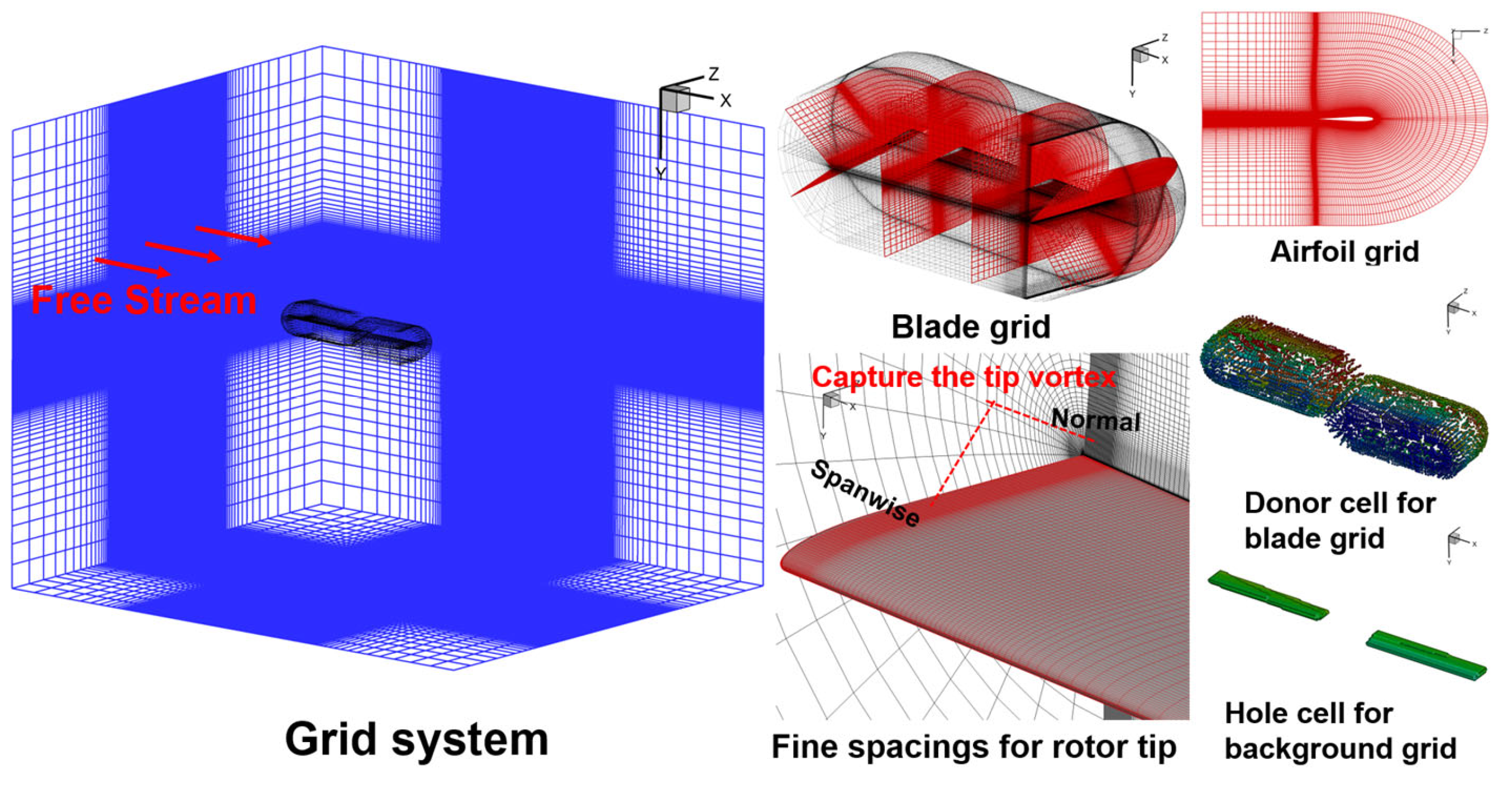
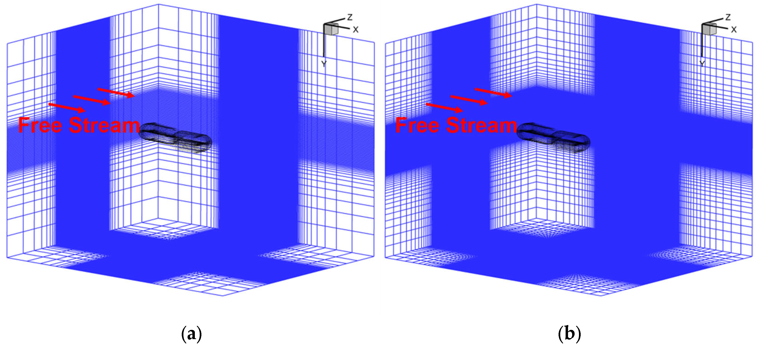
2.1. Grid System

The rotation, pitch, and flapping motions of the rotor blade are simulated using the moving overset grid method. We use the OLS rotor as an example. As shown in Figure 1, the rotor hub is the origin of the coordinate system. The incoming flow is in the x-axis direction. The +x-axis points to the rotor 0° azimuth, the +y-axis points below the rotor plane, and the +z-axis points to the rotor 90° azimuth. The distance from the wall to the outer boundary of the blade grid is 2c (c is the blade chord length), and the normal spacing at the wall is 1 × 10⁻⁵c to ensure that y⁺ < 1 on the blade surface [18,23,24]. The vortex core at the rotor tip of the blade in the normal and spanwise directions is refined with about 40 grid points, and the grid spacing in the cross-stream direction of the vortex core is 0.0025c. The results of the grid hole cells and donor cells during the CFD calculation are shown in Figure 1. The grid system of the OLS rotor consists of two C-O topology structural blade body-fitted grids and a Cartesian background grid. The blade grid and background grid are automatically generated using our self-programming meshing code [21,22] rather than commercial software. As the meshing code automatically generates the three-dimensional blade grid according to the blade-shape parameters, the coordinates of the two-dimensional airfoil structural grid are generated after inputting the airfoil coordinates. According to the blade radius, chord length distribution, and torsion distribution, the coordinates of the airfoil grid are transformed in the spanwise direction of the blade. This includes scaling, rotation, translation, and folding. Finally, the three-dimensional blade structure grid is obtained. The background grid is a cube-shaped Cartesian grid. In the forward flight case, the outer boundary length of the background grid is 7R (R represents the blade radius), 5.5R, and 6R (corresponding to the x, y, and z directions, respectively). In the hovering case, the outer boundary length of the background grid is 6R, 5.5R, and 6R, respectively. The generation of the background grid is straightforward. After dividing the grid points into the three directions, the grid point file of the background grid is automatically generated by combining the coordinate points in the three directions The blade and background grids are hexahedral. The number of blade grid points for the two-bladed OLS rotor is 225 × 80 × 155 (corresponding to the blade’s streamwise, normal, and spanwise directions, respectively), which corresponds to the conditions used in our previous studies [21,22] of blade surface blowing to reduce rotor BVI noise. Our previous research [21] showed that the computational results of the rotor wake and BVI noise sound-pressure time history were highly similar for the coarse and fine blade grids. However, the results of the rotor wake and sound pressure time history were significantly different for the coarse and fine background grids. The resolution of the background grid seemed to have a more significant effect on the accuracy of BVI noise prediction. Therefore, we use two background grid resolutions in this study to predict the BVI noise of the OLS rotor (shown in Figure 2) to analyze the effect of fine and coarse background grid resolutions on the computational accuracy of BVI noise with different numerical schemes. The fine grid has 300 × 166 × 247 background grid points (same as in the previous study [21,22]). The coarse grid uses half of the grid points of the fine grid in the three directions (150 × 83 × 123). It should be noted that the grid file generated by the meshing codes includes only the coordinates of the grid points. After the CFD code reads the grid file, it processes the data as follows. It calculates the number of cells according to the number of grid points and the surface, volume, and normal vector according to the coordinates of the grid points. The number of cells is 224 × 79 × 154 for 225 × 80 × 155 blade grid points for the two-bladed OLS rotor. The number of cells is 299 × 165 × 246 for the background grid with 300 × 166 × 247 points. In this way, we can use the cell-centered finite volume method for discretization. The Helishape-7A rotor and the UH-1H rotor are selected for testing the effectiveness of the CFD and acoustic solvers, respectively. The four-bladed Helishape-7A rotor has 225 × 80 × 177 grid points per blade, and there are 382 × 158 × 249 background grid points. The number of blade grid points used in the two-bladed UH-1H rotor is 225 × 80 × 158 per blade, and the number of background grid points is 263 × 191 × 263.

2.2. Flow Solver

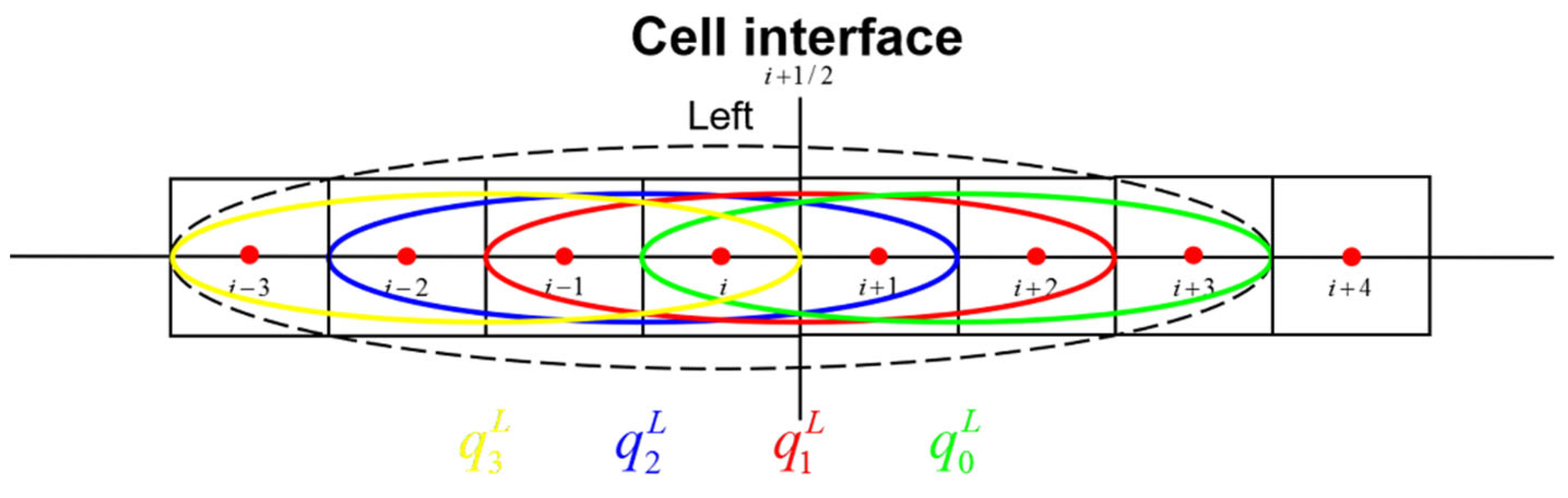
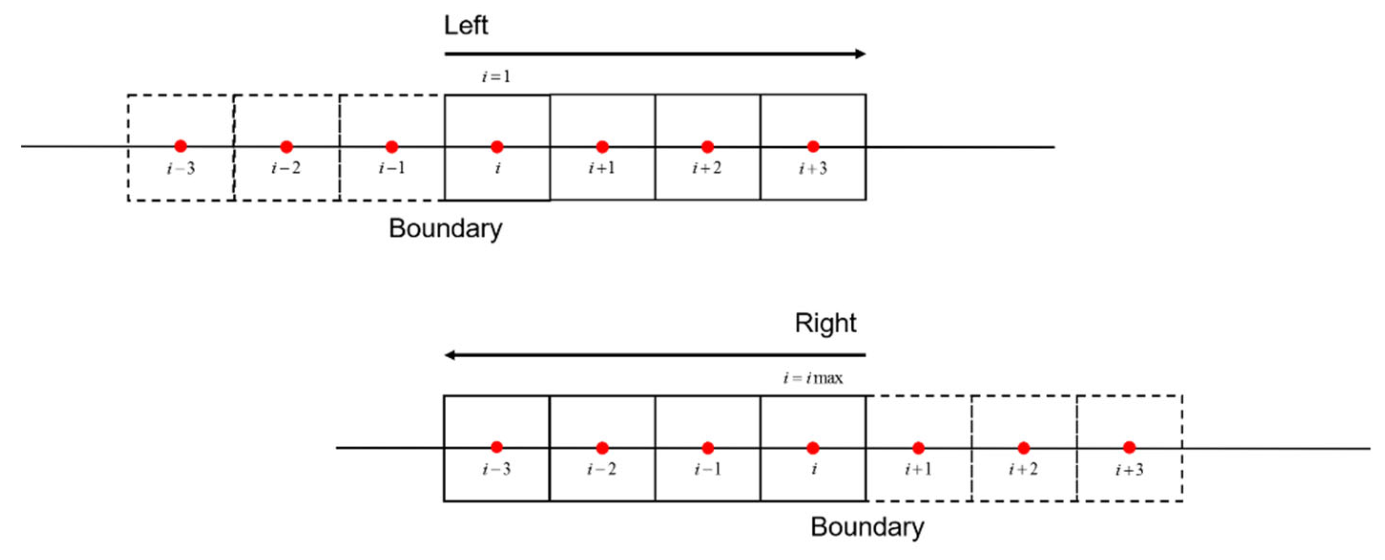
2.2.1. High-Order WENO Scheme CFD Method

The rotor flow field is solved using the latest version of the self-programming CFD codes [17,21,22,25,26], which were developed by our research group over several years. The method has been widely used and validated for simulating single/coaxial rotors during hovering and forward flight; it has good grid convergence, high computational accuracy, and high robustness. The URANS equations in the inertial coordinate system are used as the governing equations:

$$\frac{\partial }{\partial t}{\displaystyle \underset{V}{\iiint }\mathit{W}dV}+{\displaystyle \underset{\partial V}{\iint }{\mathit{F}}_c\cdot \mathit{n}dS-}{\displaystyle \underset{\partial V}{\iint }{\mathit{F}}_v\cdot \mathit{n}dS}=0$$

(1)

where $\mathit{W}$ is the vector of the conservative variables and ${\mathit{F}}_c$ and ${\mathit{F}}_v$ represent the inviscid flux and viscous flux, respectively. The detailed descriptions of these variables are given in the literature [21].

The cell-centered finite volume method is used for spatial discretization of the governing equations. The viscous flux is discretized by the second-order central difference scheme, and the inviscid flux is discretized by the Roe flux difference splitting scheme. The dual-time iteration method is used for the time advance, the implicit Lower–Upper Symmetric Gauss–Seidel (LU-SGS) scheme is used to determine the pseudo-time step, and the Spalart–Allmaras (S–A) model is selected as the turbulence model. The primitive variables on the left and right sides of the cell interface need to be reconstructed in the Roe scheme. Commonly used flow field reconstruction methods include the MUSCL and the WENO schemes. The numerical methods of the fifth-order WENO-Z scheme and the third-order MUSCL have been discussed in our previous research [21]. Thus, we only introduce the reconstruction algorithm of the seventh-order WENO-Z scheme [14,15] in the CFD solver.

Generally, the number of stencils involved in the reconstruction determines the interpolation accuracy [14,15]. The (2r-1)-point global stencil is used for the (2r-1)-order WENO scheme. It can be subdivided into r sub stencils $\left\{S_0,S_1,\dots ,S_{r-1}\right\}$ containing r grid points. As shown in Figure 3, the seven-point global stencil $S^7$ used in the seventh-order WENO scheme (in the case of r = 4) is composed of four four-point sub stencils $\left\{S_0,S_1,S_2,S_3\right\}$. We use the i-direction as an example. The left-side extrapolated values $q_{i+1/2}^L$ of the interface are given by (the right values $q_{i+1/2}^R$ can be obtained by symmetry):

$$q_{i+1/2}^L={\omega }_0{q}_0^L+{\omega }_1{q}_1^L+{\omega }_2{q}_2^L+{\omega }_3{q}_3^L$$

(2)

where $q_k^L\left(k=0,1,2,3\right)$ is obtained by the interpolations of the seven-point stencil:

$$\begin{array}{l}{q}_0^L=\frac{1}{4}{q}_i+\frac{13}{12}{q}_{i+1}-\frac{5}{12}{q}_{i+2}+\frac{1}{12}{q}_{i+3}\\ q_1^L=-\frac{1}{12}{q}_{i-1}+\frac{7}{12}{q}_i+\frac{7}{12}{q}_{i+1}-\frac{1}{12}{q}_{i+2}\\ q_2^L=\frac{1}{12}{q}_{i-2}-\frac{5}{12}{q}_{i-1}+\frac{13}{12}{q}_i+\frac{1}{4}{q}_{i+1}\\ q_3^L=-\frac{1}{4}{q}_{i-3}+\frac{13}{12}{q}_{i-2}-\frac{23}{12}{q}_{i-1}+\frac{25}{12}{q}_i\end{array}$$

(3)

The weights ${\omega }_k^z$ for the WENO-Z scheme are defined as follows:

$${\omega }_k^z=\frac{{\alpha }_k^z}{{\displaystyle \sum _{l=0}^{r-1}{\alpha }_l^z}},{\alpha }_k^z=d_k\left(1+{\left(\frac{{\tau }_{2r-1}}{{\beta }_k+\epsilon }\right)}^p\right),k=0,1,\dots r-1,$$

(4)

where ${\alpha }_k^z$ are the unnormalized weights, and ${\beta }_k$ are the smoothness indicators; ${\tau }_{2r-1}$ is simply defined as the absolute difference between ${\beta }_0$ and ${\beta }_{r-1}$, i.e., ${\tau }_{2r-1}=\left|{\beta }_0-{\beta }_{r-1}\right|$; $p\ge 1$ is used to increase the ratio between the smoothness indicators, and the small number $\epsilon$ is used to avoid division by zero in the denominators. For the seventh-order WENO scheme (in the case of r = 4), $d_0=\frac{4}{35},d_1=\frac{18}{35},d_2=\frac{12}{35},d_3=\frac{1}{35}$ are the ideal weight coefficients. The expressions of ${\beta }_k$ are given by [12]:

$$\begin{array}{l}{\beta }_0=q_i\left(2107q_i-9402q_{i+1}+7042q_{i+2}-1854q_{i+3}\right)+q_{i+1}\left(11003q_{i+1}-17246q_{i+2}+4642q_{i+3}\right)+\\ q_{i+2}\left(7043q_{i+2}-3882q_{i+3}\right)+547q_{i+3}^2\\ {\beta }_1=q_{i-1}\left(547q_{i-1}-2522q_i+1922q_{i+1}-494q_{i+2}\right)+q_i\left(3443q_i-5966q_{i+1}+1602q_{i+2}\right)+\\ q_{i+1}\left(2843q_{i+1}-1642q_{i+2}\right)+267q_{i+2}^2\\ {\beta }_2=q_{i-2}\left(267q_{i-2}-1642q_{i-1}+1602q_i-494q_{i+1}\right)+q_{i-1}\left(2843q_{i-1}-5966q_i+1922q_{i+1}\right)+\\ q_i\left(3443q_i-2522q_{i+1}\right)+547q_{i+1}^2\\ {\beta }_3=q_{i-3}\left(547q_{i-3}-3882q_{i-2}+4642q_{i-1}-1854q_i\right)+q_{i-2}\left(7043q_{i-2}-17246q_{i-1}+7042q_i\right)+\\ q_{i-1}\left(11003q_{i-1}-9402q_i\right)+2107q_i^2\end{array}$$

(5)

We use the three-layer dummy cell method [27] to process the boundary of the computational domain so that the discretization of the boundary maintains the seventh-order accuracy. The dummy cells are additional layers of grid cells outside the physical computational domain. As shown in Figure 4, a three-layer dummy cell is added outside the boundary, and the values of the primitive variables in the dummy cell are obtained by extrapolation from the interior:

$$\mathrm{Left}:q_{i-1}^D=2q_i-q_{i+1},q_{i-2}^D=3q_i-2q_{i+1},q_{i-3}^D=3q_i-q_{i+1}-q_{i+2}$$

(6)

$$\mathrm{Right}:q_{i+1}^D=2q_i-q_{i-1},q_{i+2}^D=3q_i-2q_{i-1},q_{i+3}^D=3q_i-q_{i-1}-q_{i-2}$$

(7)

The physical grid cell inside the domain starts from the left of $i=1$ and ends at the right of $i=i\max$. The following situations need to be considered:

$i=1$, the seven-point stencil is composed of four physical grid cells $q_i,q_{i+1},q_{i+2},q_{i+3}$ and three dummy cells $q_{i-1}^D,q_{i-2}^D,q_{i-3}^D$;

$i=2$, the seven-point stencil is composed of five physical grid cells $q_{i-1},q_i,q_{i+1},q_{i+2},q_{i+3}$ and two dummy cells $q_{i-1}^D,q_{i-2}^D$;

$i=3$, the seven-point stencil is composed of six physical grid cells $q_{i-2},q_{i-1},q_i,q_{i+1},q_{i+2},q_{i+3}$ and one dummy cell $q_{i-1}^D$;

$4\le i\le i\max -3$, the seven-point stencil is composed of seven physical grid cells $q_{i-3},q_{i-2},q_{i-1},q_i,q_{i+1},q_{i+2},q_{i+3}$;

$i=i\max -2$, the seven-point stencil is composed of six physical grid cells $q_{i-3},q_{i-2},q_{i-1},q_i,q_{i+1},q_{i+2}$ and one dummy cell $q_{i+1}^D$;

$i=i\max -1$, the seven-point stencil is composed of five physical grid cells $q_{i-3},q_{i-2},q_{i-1},q_i,q_{i+1}$ and two dummy cells $q_{i+1}^D,q_{i+2}^D$;

$i=i\max$, the seven-point stencil is composed of four physical grid cells $q_{i-3},q_{i-2},q_{i-1},q_i$ and three dummy cells $q_{i+1}^D,q_{i+2}^D,q_{i+3}^D$;

The j and k directions can be obtained in the same way. Thus, we ensure that the entire domain has the accuracy of the seventh-order WENO-Z scheme.

The key to simulating rotor BVI is the accurate capture of the rotor tip vortex trajectory. Thus, the resolution of the rotor wake must be high, and the CFD solver must have low numerical dissipation. Three schemes (the fifth- and seventh-order WENO-Z and the third-order MUSCL schemes) are compared in this study. The inputs of CFD code are blade grid file, background grid file, CFD configuration file (described above), and rotor motion configuration file, and the outputs include the files of the density, velocity and pressure of flow field. The CFD solver runs 4 revolutions with 1440 steps per revolution, i.e., the time step is 0.25° azimuth. The codes run on a PC with an 8-core Intel Core i7-7700 CPU (3.60 GHz) and 32.0 GB of RAM [21,22].

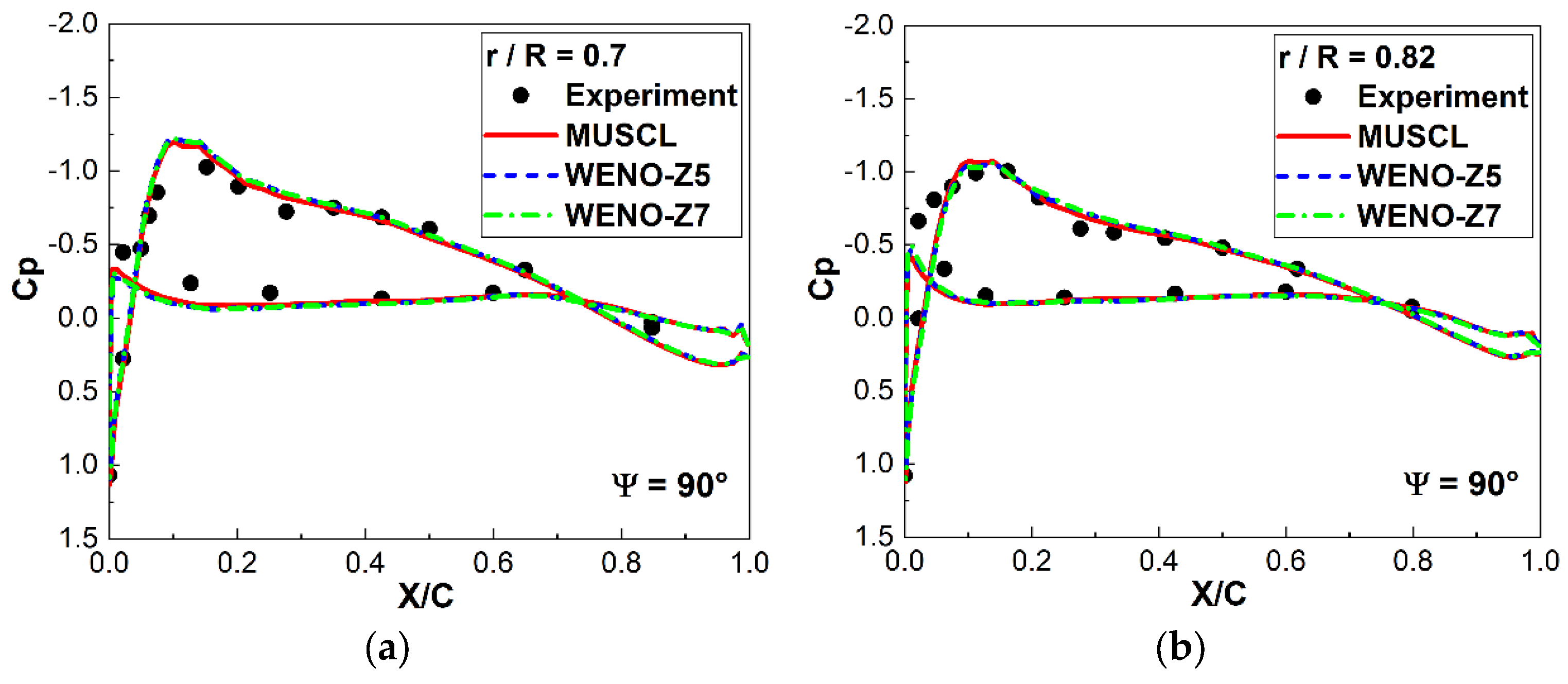
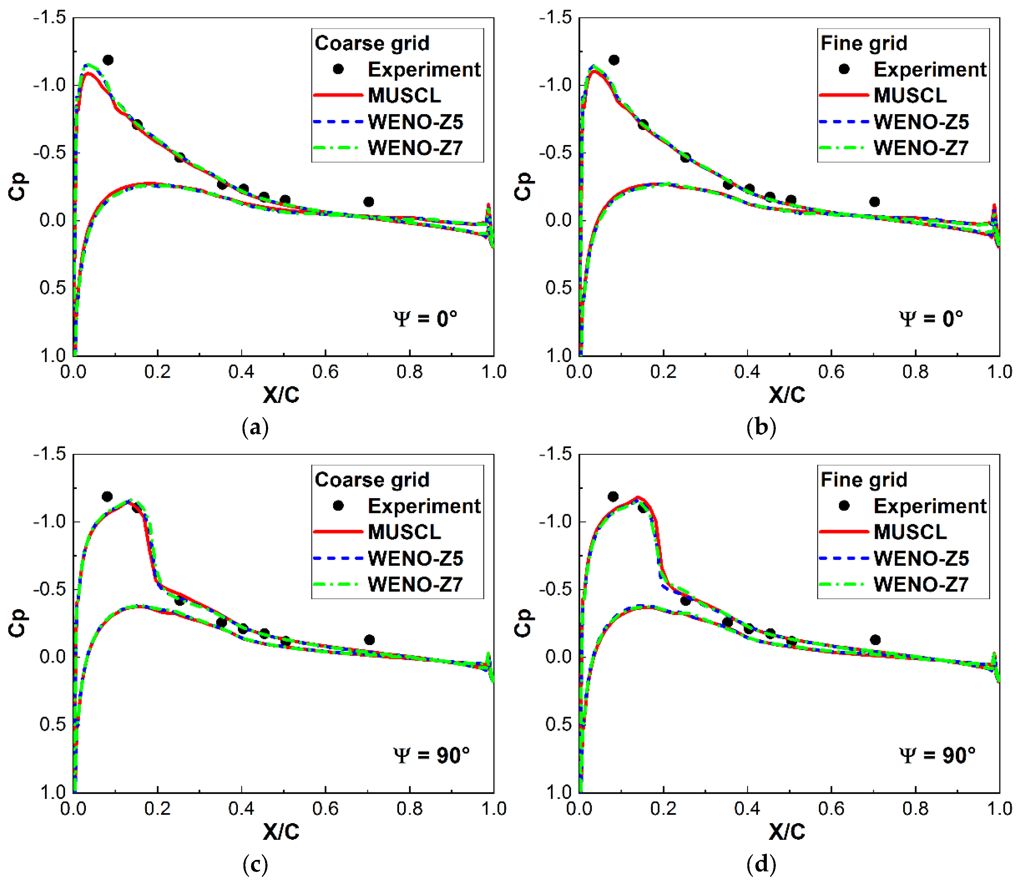
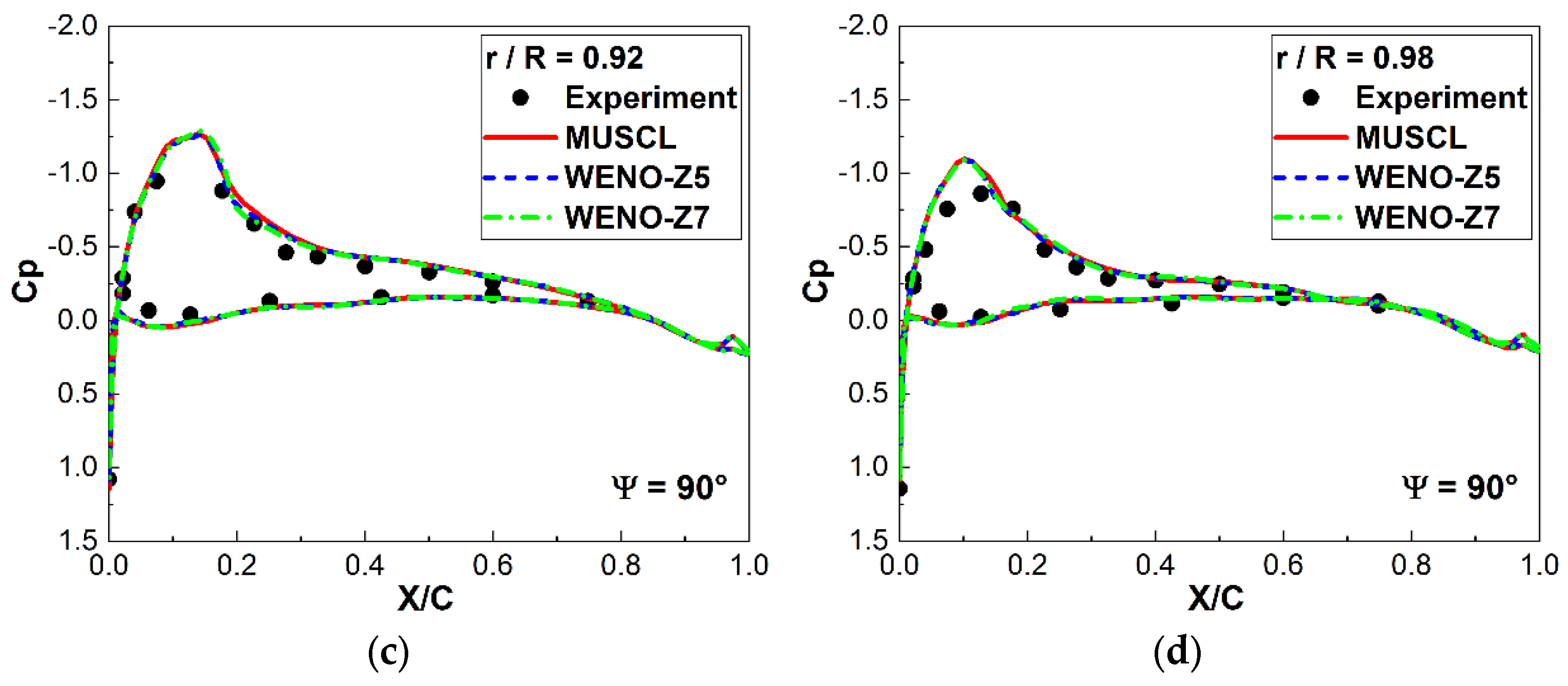
2.2.2. Numerical Validation

The Helishape-7A rotor [28] is selected to validate the experimental results of the flow solver. It consists of four blades with a blade radius of 2.1 m and a chord length of 0.14 m. It has multi-element airfoils (the OA213 airfoil is used in the inner section of the blade, and the OA209 airfoil is used in the tip section) and linear aerodynamic twist of multiple sections. The tip Mach number is 0.616, the advance ratio is 0.167, and the rotor shaft angle is 1.48° for evaluating the BVI state [29]. The fifth- and seventh-order WENO-Z and the third-order MUSCL schemes are used to simulate the flow field to evaluate the computational accuracy of the solver and compare the rotor wake resolutions of the numerical schemes.

Figure 5 shows the surface pressure coefficients in multiple spanwise sections of the blade obtained from the experiment and the fifth- and seventh-order WENO-Z and the third-order MUSCL schemes. The three schemes can accurately simulate the aerodynamics of the blade surface. The calculated surface pressure coefficients are in good agreement with the experimental data for all sections, indicating the high computation accuracy of the flow solver.

Figure 6 shows the Q criterion (Q = 0.001) for the simulated rotor wake obtained from the WENO-Z and the MUSCL schemes. Significant BVI exists in the rotor plane. The WENO and MUSCL schemes exhibit substantial differences in the wake resolution for the same grid condition. The WENO scheme is superior to the MUSCL regarding the rotor wake resolution. The WENO schemes seem to provide more details of the tip vortex structure and trajectory than the MUSCL. The seventh-order WENO scheme performs better than the fifth-order WENO scheme for maintaining the trajectory of the wake, even at about two radii downstream. However, the rotor wake simulated by the MUSCL has large dissipation and low resolution, making it difficult to capture the BVI accurately. These results demonstrate the low dissipation characteristics and high rotor wake resolution of the WENO scheme, indicating its advantages over the MUSCL for capturing the flow physics of the rotor wake and analyzing the BVI characteristics.

2.3. Acoustic Solver

2.3.1. Acoustic Method

The details of the acoustic solver have been provided in [21,22,30]. Here, we briefly review the acoustic method in our codes. The codes for predicting rotor aerodynamic noise were developed using Farassat’s Formulation 1A based on the FW–H equations based on an acoustic analogy [31,32,33]. Formulation 1A has a clear physical meaning. The blade surface is selected as the integral surface, and the total acoustic pressure is the sum of the acoustic pressure due to the thickness and loading. The specific solution of Formulation 1A is given in the literature [21,32,33]. After the calculation of the flow solver, the grid coordinates (representing the input of the thickness noise) and the pressure (representing the input of the loading noise) of the grid cells on the blade surface output by the CFD codes are used as the input of the noise solver. The acoustic pressure at the observer position can be obtained by integrating the formulation at the retarded time.

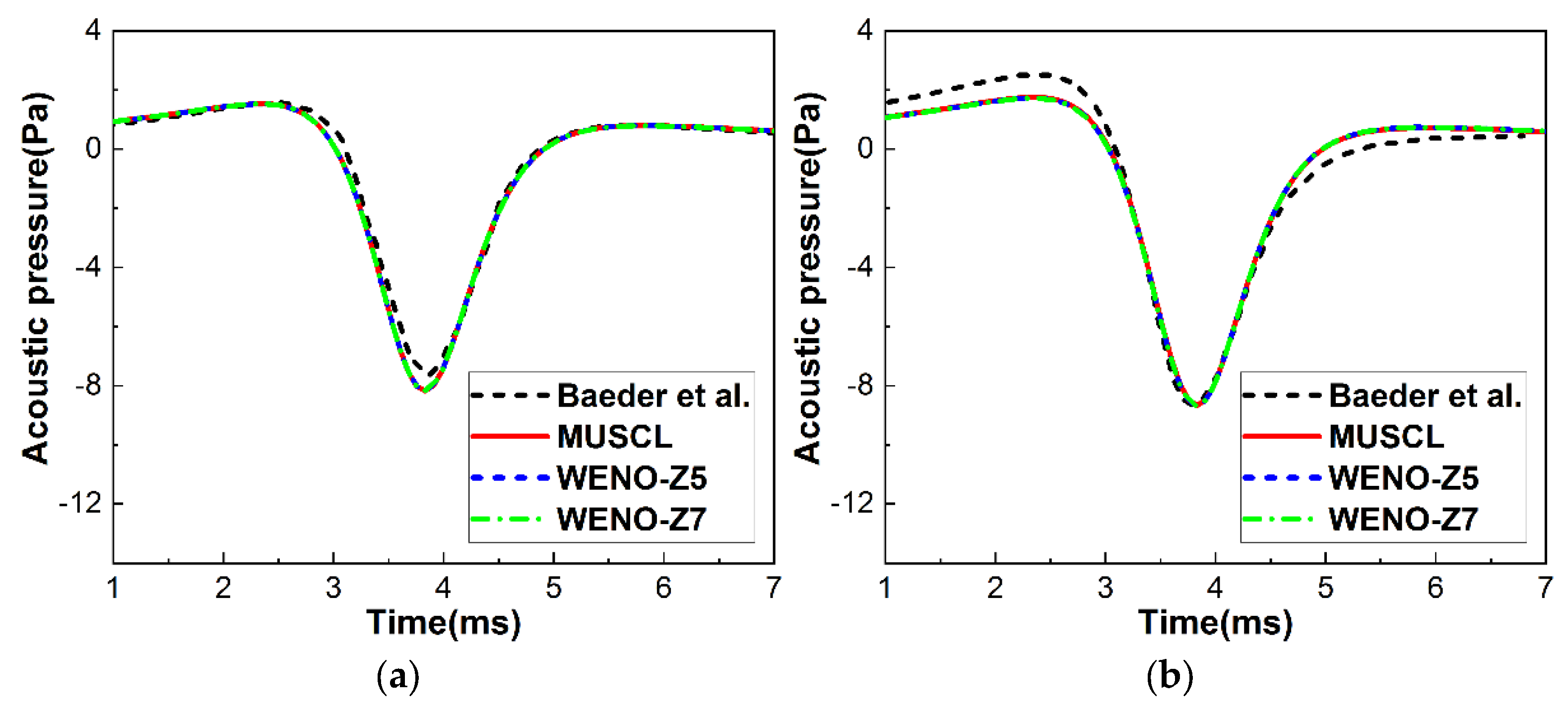
2.3.2. Numerical Validation

The UH-1H model rotor [34] is used to validate the results of the acoustic solver. It is a 1/7-scaled model of the UH-1H main rotor of the NACA0012 airfoil with two straight untwisted rectangular blades. The rotor radius is 1.045 m, and the chord length is 0.0762 m. Baeder et al. [34] used the transonic unsteady rotor Navier–Stokes (TURNS) CFD code [35] and three noise-prediction approaches [34] to investigate the aeroacoustics of the UH-1H rotor in hover. The three methods are (1) a CFD code based on the Euler equations to directly calculate the acoustic field (Euler), (2) a code based on the linear stationary Kirchhoff formulation (Euler/Kirchhoff), and (3) a code based on the linear acoustic analogy approach. (FW–H, namely, Farassat’s Formulation 1A). The Formulation 1A method can calculate the thickness noise independently, but the Euler and Euler/Kirchhoff methods can only calculate the total noise and cannot distinguish the thickness noise. The code developed based on the Formulation 1A is called the rotor acoustic prediction program (RAPP) noise code [36]. Baeder et al. [34] conducted numerical studies on the rotor noise of the UH-1H model for a wide range of hover tip Mach numbers. Here, one case investigated by Baeder et al. [34] is selected for validation. It corresponds to the non-lifting hovering state with a rotor collective pitch of zero and a tip Mach number of 0.7.

Figure 7 shows the thickness noise and total noise pressure time history in the plane of the rotor at 3.09 radii from the rotor hub for the fifth- and seventh-order WENO-Z, the third-order MUSCL schemes, and the results calculated by Baeder et al. [34]. It should be noted that the total noise result obtained by Baeder et al. was calculated by the Euler and Euler/ Kirchhoff methods, whereas the thickness noise was calculated by the RAPP code (Formulation 1A method). The thickness noise is only related to the blade geometry and does not depend on the CFD code. The thickness noise can be obtained independently by inputting the coordinates of the grid points on the blade surface; thus, the thickness noise is the same for each scheme because the same grid is used. Our results of the thickness noise are consistent with the prediction by the RAPP code regarding the waveform and phase. Therefore, the noise calculation method (Formulation 1A method) we use is consistent with that of Bader et al. for comparing the thickness noise; thus, the waveforms are similar. There are slight overestimations in the negative pressure peak compared to Baeder et al. [34], which may be because Baeder et al. used different blade grids. The total noise is calculated by using the grid-point coordinates, and the aerodynamic load on the blade surface is calculated by the CFD code as the input of the noise code. The aerodynamic load is very small since there is no lift, and the thickness noise dominates the total noise. Therefore, the total noise calculated by the three schemes is similar. Since the calculation method of the total noise we use is different from that of Baeder et al. [34], it is difficult to compare the waveform. However, the similar amplitudes indicate the applicability of our acoustic solver.

3. BVI Noise Prediction

The OLS rotor aerodynamic/noise test results [8,37] obtained in the German–Dutch wind tunnel (DNW) are used for the prediction of BVI noise. The OLS rotor is a 1/7-scaled model rotor of the AH-1 helicopter main rotor. It has two rectangular OLS airfoil blades. The rotor radius is 0.958 m, and the chord length is 0.1039 m. The blade has an 8.2° negative twist from root to tip. The 10014 test case [8,35] under low-speed descent flight is selected in this study. The tip Mach number is 0.664, and the advance ratio is 0.164. Although the rotor shaft angle is 0°, the rotor tip-path plane angle is tilted backward 1° due to the adjustment of longitudinal flapping in the test. Three microphones (3, 7, and 9) are used in the test to measure the BVI noise signal. Their locations are the observer position for noise prediction. The three microphones are installed at 30° below the rotor plane and at 3.44 radii from the rotor hub, and the azimuth angles are 180°, 150°, and 210°, respectively. The microphone coordinates are listed in

Table 1. Locations of microphones 3, 7, and 9 in the experiment (normalized by the chord length).

Microphone	x	y	z
3	−27.467	15.858	0.0
7	−23.787	15.858	13.733
9	−23.787	15.858	−13.733

(normalized by the chord length) [8].

The fifth- and seventh-order WENO and MUSCL schemes are used to simulate the rotor flow field for the coarse and fine grids. The grid coordinates and the aerodynamic load of the blade surface calculated by the CFD code are used as the input of the noise code to predict the BVI noise. The computational accuracy of the three schemes for the flow field simulation and BVI noise prediction for the coarse and fine grids are compared with the experimental results.

Figure 8 shows the blade pressure coefficients at the spanwise 0.955R position at azimuths of 0°, 90°, and 180° of for the coarse and fine grids obtained from the experiment [8] and the three schemes. The pressure coefficients calculated by the three schemes are in good agreement with the experimental data for both grid resolutions. Only the MUSCL underestimates the negative pressure peak near the leading edge of the blade’s upper surface in the coarse grid. The negative pressure peak predicted by the WENO schemes for the coarse and fine grid cases is closer to the experimental results than that of the MUSCL scheme. Overall, the surface pressure coefficients are accurately predicted by the flow solver.

Figure 9 shows the rotor wake results of the iso-surfaces of the Q criterion (Q = 0.001) at the 90° azimuth obtained from the three schemes for the coarse and fine grids. There is a significant difference in the simulation resolution of the rotor wake between the three schemes. The WENO schemes seem to have a better capture resolution on the induced vortical structures than the MUSCL for the coarse and fine grids. The resolution for capturing the BVI in the rotor plane is higher, and the seventh-order WENO scheme captures more vortex sheets in the rotor plane. The wake system simulated by the MUSCL exhibits large numerical dissipation, even for the fine grid. The wake resolution of the MUSCL for the fine grid case is equivalent to that of the WENO scheme for the coarse grid. These results demonstrate the effectiveness of the WENO scheme for reducing the numerical dissipation of the rotor wake, indicating that this scheme provides better performance for simulating the rotor wake and the rotor BVI characteristics than the MUSCL.

Figure 10 shows the noise pressure time history obtained from the experiment [8] with microphones 3, 7, and 9, and the three schemes. The pulse waveform and phase of the BVI noise predicted by the WENO scheme for the fine grid are consistent with the experimental data. The pulse fluctuation characteristics of the BVI noise are well resolved, and the peak sound-pressure of the BVI noise is accurately predicted. Although the calculation results differ from the experimental results for the coarse grid due to the low grid resolution, the peak sound-pressure of the seventh-order WENO scheme is closer to the experimental data than that of the fifth-order WENO scheme. In contrast, the pulse shape and amplitude predicted by the MUSCL for both grids do not agree with the experimental data. The predicted BVI noise peak has considerable error compared with the test data, even for the fine grid. Thus, the peak sound-pressure cannot be predicted accurately by the MUSCL. The difference in the calculation results of the sound-pressure peak shows that the high-order WENO scheme has less numerical dissipation and significantly higher prediction accuracy for the BVI noise than the MUSCL. Although the calculation results capture the dominant vortex-induced pulse fluctuations of the BVI noise, the accuracy of the small fluctuations in the sound pressure is not sufficient for some azimuth phases. The small load fluctuations may have been caused by the elastic deformation of the blade. The proposed numerical method does not include computational structural dynamics (CSD) modeling and cannot simulate blade deformation. The accurate prediction of BVI noise is a challenging problem in rotor aerodynamics and aeroacoustics. The flow solver requires a high-order scheme with low dissipation characteristics and should simulate the elastic deformation of the blades. In future research, we will develop a CFD/CSD code based on the aeroelastic coupling to improve the noise-prediction accuracy.

Table 2. Comparisons of the computational costs and SPLs of the WENO-Z and the MUSCL schemes for coarse and fine grids.

Case	Numerical Scheme	CPUh/rev	SPL (dB)
			MIC 3	MIC 7	MIC 9
Coarse grid	MUSCL	150.2	108.414	105.344	107.705
	WENO-Z5	191.4	109.192	106.405	108.361
	WENO-Z7	195.3	110.073	107.072	109.364
Fine grid	MUSCL	333.1	109.816	107.786	108.434
	WENO-Z5	640.0	110.326	106.535	110.373
	WENO-Z7	680.8	110.747	106.920	111.040

lists the computational cost and the computed sound-pressure level (SPL) of the fifth- and seventh-order WENO schemes and the third-order MUSCL for simulating the BVI of the OLS rotor. The computational cost is a critical issue in CFD simulations of rotor dynamics. The computational time of the MUSCL is 150.2 CPU hours per rotor revolution for MUSCL and 191.4 and 195.3 CPU hours for the fifth- and seventh-order WENO schemes, respectively, for the coarse grid. For the fine grid, the times are 333.1 h, 640.0 h, and 680.8 h for the MUSCL and the fifth- and seventh order WENO schemes, respectively. The computational cost of the WENO scheme is higher than that of the MUSCL for the same grid condition, and the computational cost increases significantly with the grid resolution. The computational cost of the WENO scheme is 30% higher than that of the MUSCL for the coarse grid case and twice as high for the fine grid. Since WENO-Z5 and WENO-Z7 have similar equations, only the number of the chosen templates is different. The equations only differ in the number of terms, but the power level is the same. Therefore, the computational time is similar. In contrast, the MUSCL method is relatively simple; thus, the computational time is less than that of the WENO schemes. Because the experimental data of the SPLs at the microphones are not provided in the literature [8], we can only compare the computed results of the SPLs for the schemes. The SPL calculation results of WENO-Z5 and WENO-Z7 are very similar, but the differences in the calculation results of MUSCL are more than 1 dB. This result is consistent with the difference between the sound-pressure time-history calculations. Although the MUSCL is more efficient than the WENO scheme, it has low accuracy for simulating the rotor wake in the BVI state and is unsuitable for rotor BVI noise prediction. The WENO scheme has a significantly higher resolution of the rotor wake and higher prediction accuracy of the BVI noise than the MUSCL. The calculated BVI sound-pressure peak is consistent with the experimental results. The seventh-order WENO scheme has the highest prediction accuracy for both grids. The wake simulation resolution and noise calculation results of the MUSCL with the fine grid are equivalent to those of the WENO schemes with the coarse grid. Therefore, the WENO schemes can predict BVI using a coarser grid than the MUSCL. In this case, the computational cost of the WENO schemes is relatively low (195.3 vs. 333.1 CPUh/rev). Our calculations were performed on a PC with limited computational resources. The relatively low computational cost due to the coarser grid and relatively high accuracy of the WENO schemes are advantageous for CFD simulations of rotor BVI on a standard PC. Our previous research [21] also showed that for the same computational cost (time), the WENO scheme with a coarse grid performed better than the MUSCL with a fine grid for capturing the vortex and predicting BVI noise. The computational cost of WENO increases significantly as the grid scale increases. We plan to develop more efficient parallel acceleration techniques in the CFD code to reduce the computational cost of high-order WENO schemes. We also hope to use a supercomputer or computing clusters in a future BVI study to analyze data with a higher resolution.

4. Conclusions

This paper proposed a high-resolution CFD/FW–H method for rotor BVI noise prediction based on high-order WENO schemes. The seventh-order WENO-Z scheme was used with the CFD method, and three-layer dummy cells were implemented at the boundary of the computational domain to ensure that the flux at the boundary maintained the seventh-order accuracy. The rotor flow field, the BVI noise-prediction accuracy, and the computational cost of the fifth- and seventh-order WENO schemes were compared with that of the third-order MUSCL for coarse and fine grids. The conclusions are as follows:

(1)

The flow solver based on the URANS method and the acoustic solver based on the FW–H method exhibited high computational accuracy, demonstrating their suitability for rotor flow field simulation and noise prediction.

(2)

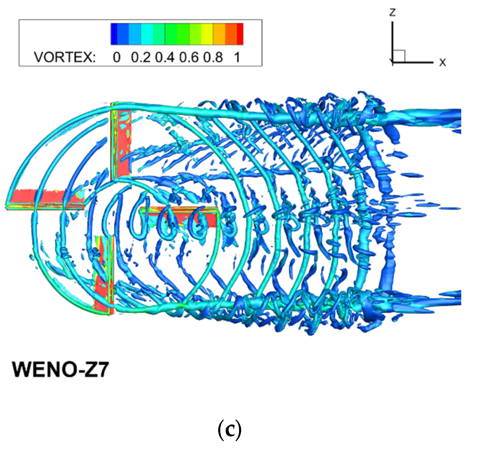
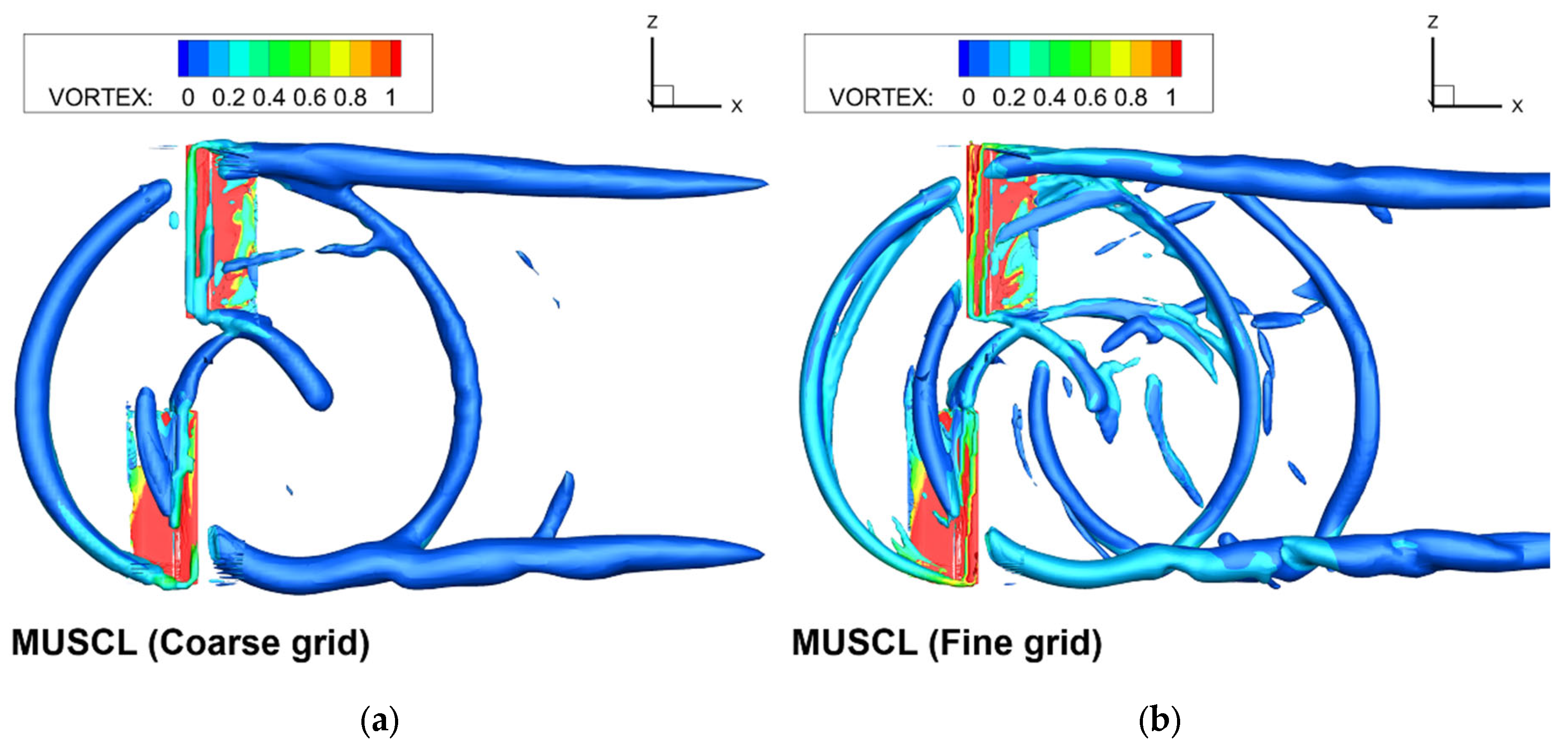
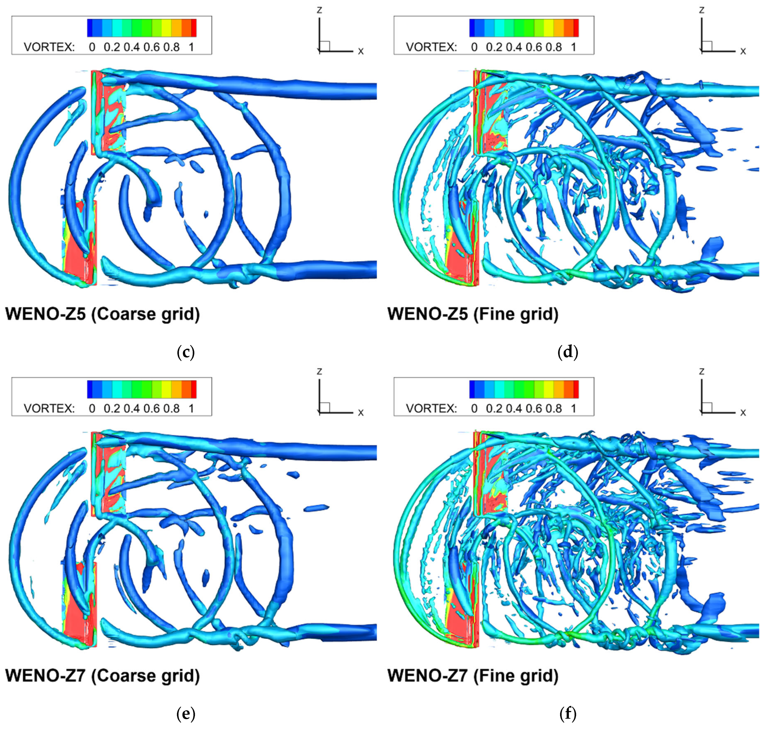
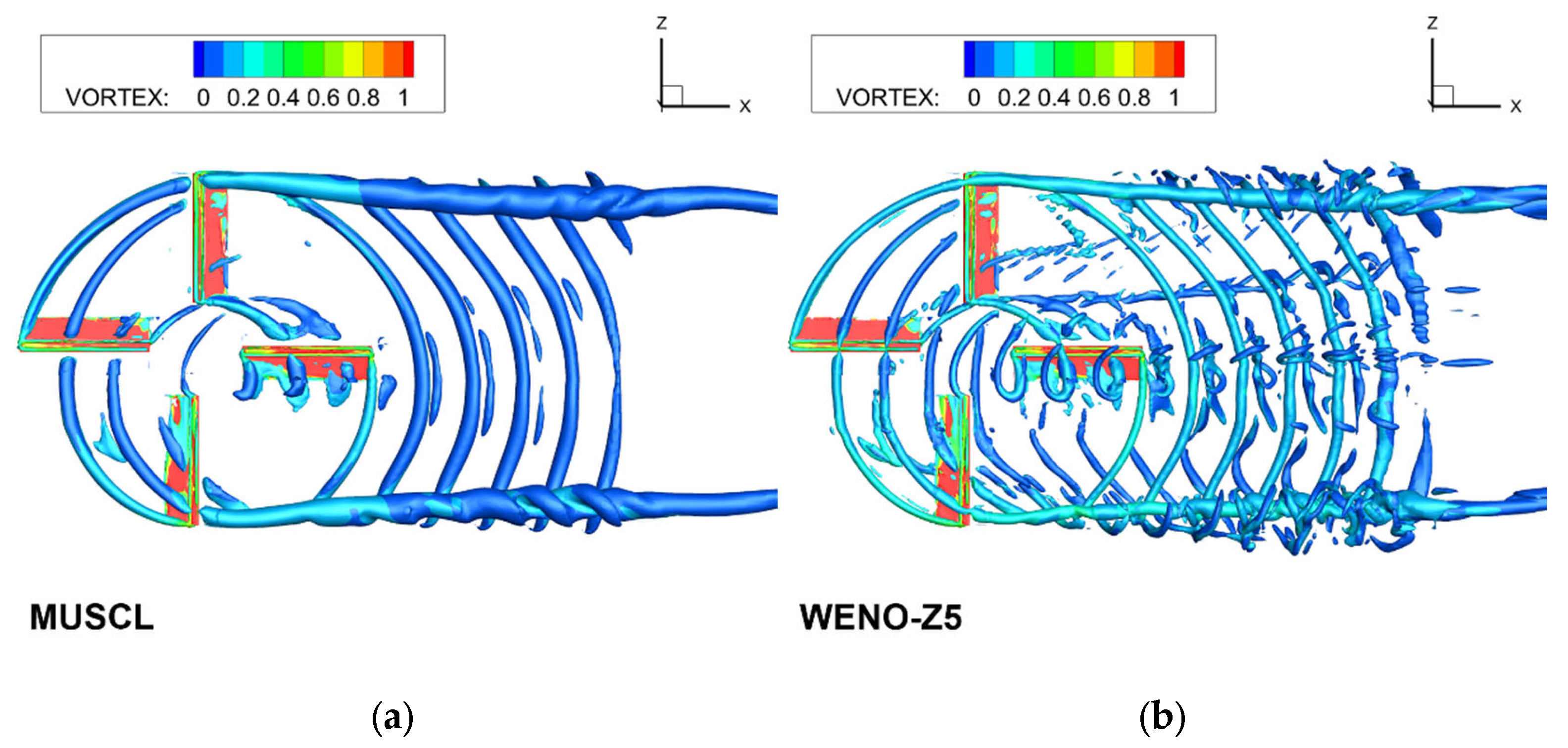
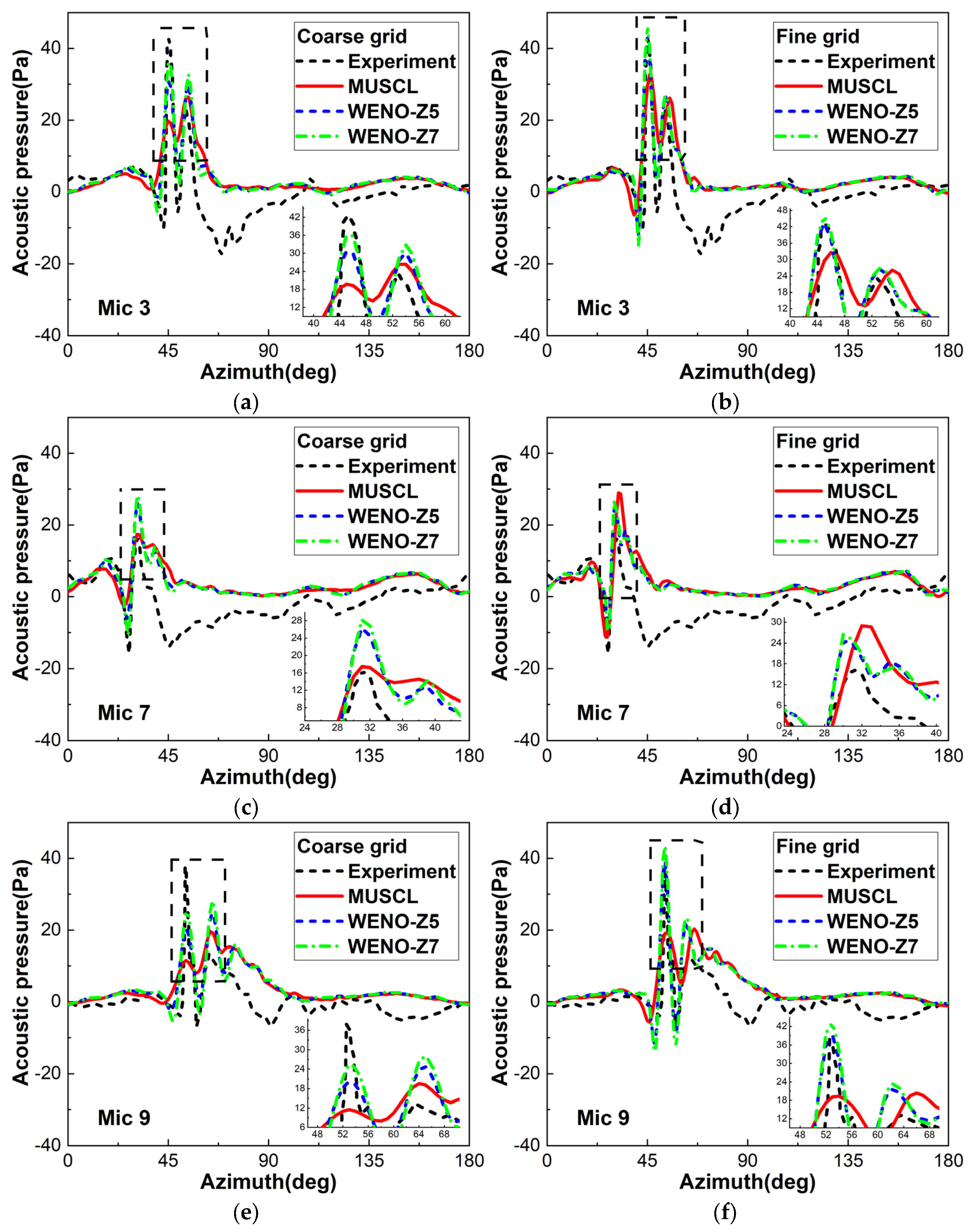
The CFD/FW–H method based on the high-order WENO scheme had higher wake resolution and significantly higher BVI noise-prediction accuracy than the MUSCL scheme.

(3)

The WENO scheme exhibited low dissipation of the numerical characteristics, improving the rotor wake simulation results and the pulse characteristics and peaks of the BVI noise. The seventh-order scheme showed higher simulation accuracy than the fifth-order scheme. In contrast, the wake simulated by the MUSCL has excessive dissipation, and the prediction accuracy for BVI noise was low for both grids. The wake resolution of the MUSCL for the fine grid was equivalent to that of the WENO scheme for the coarse grid.

(4)

The computational cost of the WENO scheme was higher than that of the MUSCL for the same grid resolution. The computational cost of the seventh-order WENO scheme was higher than that of the fifth-order WENO scheme, indicating an increase in the computational cost with the grid resolution. The computational cost of the WENO scheme was 30% higher than that of the MUSCL for the coarse grid and twice as high for the fine grid.

(5)

The WENO schemes can predict BVI using a coarser grid than the MUSCL. In this case, the computational cost of the WENO schemes is relatively low. The relatively low computational cost due to the coarser grid and relatively high accuracy of the WENO schemes are advantageous for CFD simulations of rotor BVI on a standard PC.

The authors plan to improve the numerical methods for predicting BVI noise. We will develop a more efficient parallel acceleration method in the CFD code to reduce the computational cost of the WENO scheme and improve computational efficiency. We also plan to develop a CFD/CSD code using aeroelastic coupling modeling to improve the BVI noise-prediction accuracy. Large Eddy Simulation (LES) is an important development direction to systematically predict rotor aerodynamic noise in the future. We also hope to have the opportunity to use a supercomputer or computing clusters in a future BVI study to analyze data with a higher resolution.

References

1. Preisser, J.S.; Brooks, T.F.; Martin, R.M. Recent studies of rotorcraft blade-vortex interaction noise. J. Aircr. 1994, 31, 1009–1015. [Google Scholar] [CrossRef]
2. Huang, Z.; Siozos-Rousoulis, L.; De Troyer, T.; Ghorbaniasl, G. Helicopter rotor noise prediction using a convected FW-H equation in the frequency domain. Appl. Acoust. 2018, 140, 122–131. [Google Scholar] [CrossRef]
3. Vouros, S.; Goulos, I.; Pachidis, V. Integrated methodology for the prediction of helicopter rotor noise at mission level. Aerosp. Sci. Technol. 2019, 89, 136–149. [Google Scholar] [CrossRef]
4. Jia, Z.; Lee, S. Aerodynamically induced noise of a lift-offset coaxial rotor with pitch attitude in high-speed forward flight. J. Sound Vib. 2021, 491, 115737. [Google Scholar] [CrossRef]
5. Yu, Y.H. Rotor blade-vortex interaction noise. Prog. Aerosp. Sci. 2000, 36, 97–115. [Google Scholar] [CrossRef]
6. Thom, A.; Duraisamy, K. High-resolution simulations of parallel blade–vortex interactions. AIAA J. 2010, 48, 2313–2324. [Google Scholar] [CrossRef]
7. Romani, G.; Casalino, D. Rotorcraft blade-vortex interaction noise prediction using the Lattice-Boltzmann method. Aerosp. Sci. Technol. 2019, 88, 147–157. [Google Scholar] [CrossRef]
8. Strawn, R.C.; Duque, E.P.N.; Ahmad, J. Rotorcraft aeroacoustics computations with overset-grid CFD methods. In Proceedings of the 54th American Helicopter Society Annual Forum, Washington, DC, USA, 22–24 May 1998. [Google Scholar]
9. Gennaretti, M.; Bernardini, G.; Serafini, J.; Romani, G. Rotorcraft comprehensive code assessment for blade–vortex interaction conditions. Aerosp. Sci. Technol. 2018, 80, 232–246. [Google Scholar] [CrossRef]
10. Liu, X.; Osher, S.; Chan, T. Weighted essentially non-oscillatory schemes. J. Comput. Phys. 1994, 115, 200–212. [Google Scholar] [CrossRef] [Green Version]
11. Jiang, G.; Shu, C. Efficient implementation of weighted ENO schemes. J. Comput. Phys. 1996, 126, 202–228. [Google Scholar] [CrossRef] [Green Version]
12. Balsara, D.S.; Shu, C. Monotonicity preserving weighted essentially non-oscillatory schemes with increasingly high order of accuracy. J. Comput. Phys. 2000, 160, 405–452. [Google Scholar] [CrossRef] [Green Version]
13. Xu, L.; Weng, P. High order accurate and low dissipation method for unsteady compressible viscous flow computation on helicopter rotor in forward flight. J. Comput. Phys. 2014, 258, 470–488. [Google Scholar] [CrossRef]
14. Borges, R.; Carmona, M.; Costa, B.; Don, W.S. An improved weighted essentially non-oscillatory scheme for hyperbolic conservation laws. J. Comput. Phys. 2008, 227, 3191–3211. [Google Scholar] [CrossRef]
15. Castro, M.; Costa, B.; Don, W.S. High order weighted essentially non-oscillatory WENO-Z schemes for hyperbolic conservation laws. J. Comput. Phys. 2011, 230, 1766–1792. [Google Scholar] [CrossRef]
16. Van Leer, B. Towards the ultimate conservative difference scheme. V. A second-order sequel to Godunov’s method. J. Comput. Phys. 1979, 32, 101–136. [Google Scholar] [CrossRef]
17. Ye, Z.; Zhan, F.; Xu, G. Numerical research on the unsteady evolution characteristics of blade tip vortex for helicopter rotor in forward flight. Int. J. Aeronaut. Space Sci. 2020, 21, 865–878. [Google Scholar] [CrossRef]
18. Ricci, F.; Silva, P.A.S.F.; Tsoutsanis, P.; Antoniadis, A.F. Hovering rotor solutions by high-order methods on unstructured grids. Aerosp. Sci. Technol. 2020, 97, 105648. [Google Scholar] [CrossRef]
19. Petermann, J.; Jung, Y.S.; Baeder, J.; Rauleder, J. Validation of higher-order interactional aerodynamics simulations on full helicopter configurations. J. Am. Helicopter Soc. 2019, 64, 042002. [Google Scholar] [CrossRef]
20. Yeshala, N.; Egolf, T.A.; Vasilescu, R.; Sankar, L.N. Application of higher order spatially accurate schemes to rotors in hover. In Proceedings of the 24th AIAA Applied Aerodynamics Conference, San Francisco, CA, USA, 5–8 June 2006. [Google Scholar]
21. Sun, Y.; Xu, G.; Shi, Y. Numerical investigation on noise reduction of rotor blade-vortex interaction using blade surface jet blowing. Aerosp. Sci. Technol. 2021, 116, 106868. [Google Scholar] [CrossRef]
22. Sun, Y.; Xu, G.; Shi, Y. Parametric effect of blade surface blowing on the reduction of rotor blade–vortex interaction noise. J. Aerosp. Eng. 2022, 35, 04021110. [Google Scholar] [CrossRef]
23. Strawn, R.C.; Caradonna, F.X.; Duque, E. 30 Years of Rotorcraft Computational Fluid Dynamics Research and Development. J. Am. Helicopter Soc. 2006, 51, 5–21. [Google Scholar] [CrossRef]
24. Duraisamy, K. Studies in Tip Vortex Formation, Evolution and Control. Ph.D. Thesis, University of Maryland, College Park, MD, USA, 2005. [Google Scholar]
25. Ye, Z.; Xu, G.; Shi, Y. High-resolution simulation and parametric research on helicopter rotor vortex flowfield with TAMI control in hover. Proc. Inst. Mech. Eng. Part G J. Aerosp. Eng. 2018, 232, 2513–2526. [Google Scholar] [CrossRef]
26. Qi, H.; Xu, G.; Lu, C.; Shi, Y. A study of coaxial rotor aerodynamic interaction mechanism in hover with high-efficient trim model. Aerosp. Sci. Technol. 2019, 84, 1116–1130. [Google Scholar] [CrossRef]
27. Blazek, J. Computational Fluid Dynamics: Principles and Applications, 3rd ed.; Elsevier: Kidlington, UK, 2007; pp. 253–278. [Google Scholar]
28. Steijl, R.; Barakos, G.; Badcock, K. A framework for CFD analysis of helicopter rotors in hover and forward flight. Int. J. Numer. Methods Fluids 2006, 51, 819–847. [Google Scholar] [CrossRef]
29. Biava, M.; Bindolino, G.; Vigevano, L. Single blade computations of helicopter rotors in forward flight. In Proceedings of the 41st Aerospace Sciences Meeting and Exhibit, Reno, NV, USA, 6–9 January 2003. [Google Scholar]
30. Shi, Y.; Zhao, Q.; Xu, G. An analytical study of parametric effects on rotor–vortex interaction noise. Proc. Inst. Mech. Eng. Part G J. Aerosp. Eng. 2011, 225, 259–268. [Google Scholar] [CrossRef]
31. Ffowcs Williams, J.E.; Hawkings, D.L. Sound generation by turbulence and surfaces in arbitrary motion. Philos. Trans. R. Soc. Lond. Ser. A Math. Phys. Sci. 1969, 264, 321–342. [Google Scholar]
32. Farassat, F. Linear acoustic formulas for calculation of rotating blade noise. AIAA J. 1981, 19, 1122–1130. [Google Scholar] [CrossRef]
33. Brentner, K.S.; Farassat, F. Modeling aerodynamically generated sound of helicopter rotors. Prog. Aerosp. Sci. 2003, 39, 83–120. [Google Scholar] [CrossRef] [Green Version]
34. Baeder, J.D.; Gallman, J.M.; Yu, Y.H. A computational study of the aeroacoustics of rotors in hover. In Proceedings of the 49th American Helicopter Society Annual Forum, St. Louis, MO, USA, 19–21 May 1993. [Google Scholar]
35. Srinivasan, G.R.; Baeder, J.D.; Obayashi, S.; McCroskey, W.J. Flowfield of a lifting rotor in hover: A Navier-Stokes simulation. AIAA J. 1992, 30, 2371–2378. [Google Scholar] [CrossRef]
36. Gallman, J.M. The Validation and Application of a Rotor Acoustic Prediction Computer Program; NASA-TM-101794; NASA: Washington, DC, USA, 1990.
37. Yu, Y.H.; Tung, C.; Gallman, J.; Schultz, K.J.; van der Wall, B.; Spiegel, P.; Michea, B. Aerodynamics and acoustics of rotor blade-vortex interactions. J. Aircr. 1995, 32, 970–977. [Google Scholar] [CrossRef]
Figure 1. Moving overset grid system of the OLS rotor.
Aerospace 09 00196 g001
Figure 2. Coarse and fine background grids of the OLS rotor: (a) Coarse grid case; (b) fine grid case.
Aerospace 09 00196 g002
Figure 3. Sketch of a 7-point stencil for computing the left primitive variables.
Aerospace 09 00196 g003
Figure 4. Sketch of the three-layer dummy cell.
Aerospace 09 00196 g004
Figure 5. The pressure coefficients of the Helishape-7A rotor blade section for the WENO-Z and the MUSCL schemes: (a) ψ = 90° (r/R = 0.7); (b) ψ   = 90° (r/R = 0.82); (c) ψ   = 90° (r/R = 0.92); (d) ψ   = 90° (r/R = 0.98).
Aerospace 09 00196 g005aAerospace 09 00196 g005b
Figure 6. The iso-surfaces of the Q criterion at Q = 0.001 (colored by the vorticity magnitude) of the Helishape-7A rotor for the WENO-Z and the MUSCL schemes: (a) MUSCL; (b) WENO-Z5; (c) WENO-Z7.
Aerospace 09 00196 g006aAerospace 09 00196 g006b
Figure 7. Comparison of the sound-pressure time history in the plane of the rotor at 3.09 radii of the UH-1H model rotor for the WENO-Z and the MUSCL schemes: (a) Thickness noise; (b) total noise.
Aerospace 09 00196 g007
Figure 8. The pressure coefficients of the OLS rotor blade (r/R = 0.955) for the coarse and fine grids obtained from the experiment and the WENO and MUSCL schemes: (a) ψ = 0° (coarse grid); (b) ψ = 0° (fine grid); (c) ψ = 90° (coarse grid); (d) ψ = 90° (fine grid); (e) ψ = 180° (coarse grid); (f) ψ = 180° (fine grid).
Aerospace 09 00196 g008aAerospace 09 00196 g008b
Figure 9. The iso-surfaces of the Q criterion at Q = 0.001 (colored by vorticity magnitude) of the OLS rotor for the WENO-Z and the MUSCL schemes for the coarse and fine grids: (a) MUSCL (coarse grid); (b) MUSCL (fine grid); (c) WENO-Z5 (coarse grid); (d) WENO-Z5 (fine grid); (e) WENO-Z7 (coarse grid); (f) WENO-Z7 (fine grid).
Aerospace 09 00196 g009aAerospace 09 00196 g009b
Figure 10. The BVI noise pressure time history of the OLS rotor for the WENO-Z and the MUSCL schemes for the coarse and fine grids: (a) Microphone 3 (coarse grid); (b) microphone 3 (fine grid); (c) microphone 7 (coarse grid); (d) microphone 7 (fine grid); (e) microphone 9 (coarse grid); (f) microphone 9 (Fine grid).
Aerospace 09 00196 g010