1. Introduction
The Moon is rich in minerals and energy resources and has been one of the most attractive destinations for space exploration [
1]. As a specialized mobile robot on the lunar surface, the lunar rover can adapt to the harsh environment, cross obstacles, and bear large loads [
2]. Therefore, it plays a prominent role in lunar exploration and has been widely used in plenty of lunar missions. The former Soviet Union’s lunar probes “Luna 11” and “Lunar 21” carried lunar rovers, which completed tasks including lunar reconnaissance, topographic photography, and mineral composition analysis with various scientific instruments [
3]. The “Apollo 15” and “Apollo 16” of the United States carried manned lunar rovers [
4]. Recently, China launched two lunar rovers the “Yutu” and “Yutu-2”, to detect the lunar surface [
5]. In the near future, more missions including lunar rovers have been proposed, for instance, the USA’s Artemis and China’s lunar program IV, for more thorough exploitation and utilization of the lunar resources [
6].
Generally, the lunar surface exploration is carried out based on the information of the lunar environment after a safe landing. Common exploration tasks include a geological survey of the lunar surface, soil sampling, rock mineral analysis, etc., and the process of them is mainly divided into four steps:
Perception of the lunar environment. It mostly relies on satellites and the vehicular cameras to gather information about the lunar environment, from which a digital elevation model (DEM) is generated that includes details like rocks, craters, slopes, etc. [
7].
Selection of the detecting point. A suitable target detecting point is usually selected based on the information of the lunar environment and the structure of the lunar rover.
Path planning. The path of the rover is planned in the safe area to ensure the arrival at the detecting point, in which the key is the avoidance of obstacles.
Execution of the detecting task. After the arrival of the target point, sampling and other scientific missions are carried out by using the sampling manipulator and other scientific instruments.
Normally, the first three steps are performed by the rover, while the fourth step is executed by the manipulator, which is beyond the scope of this study. In recent years, the perception technology of the surface environment has made great progress, and can be conducted with high precision [
8]. However, the selection of the detecting point and path planning for the lunar rover still mainly rely on manual control from ground personnel, which makes it inefficient to transmit large amounts of surrounding information and path planning data between the lunar rover and the ground console. Moreover, due to the time delay of transmission between the Moon and the Earth, the manual command of the ongoing task may violate the feasibility in the unstructured lunar surface environment, and even threaten the lunar rover’s security [
9]. In recent years, plenty of research has been carried out on these two abovementioned topics.
For the selection of the detecting point, to ensure it is appropriate and reachable, the safe zone for the rover’s motion should be determined first. For this purpose, Li [
10] analyzed the safe zone by extracting the topographic slope of the lunar surface. Garrido [
11] solved the safe zone by calculating the maximum and minimum slope based on the tensorial way at any point on the lunar surface. Zhou [
12] generated the goodness raster map based on the slope cost function to solve the safe zone. These studies analyzed the safe zone for rover’s motion only based on slope, while small obstacles, which cannot be expressed by the slope, are eliminated macroscopically. Moreover, the energy consumption of those small obstacles is ignored for the selection of a detecting point within the obtained safe zone. Kose [
13] chose it according to the illumination requirements of the Raman spectrometer, while Hewitt [
14] selected it by analyzing the topographic features of each grid in the raster map, such as point variance, average height, etc. The abovementioned studies consider the equipment requirements or terrain features separately, which are not feasible for the actual task because the real lunar environments are complex.
Once the detecting point is selected, a safe path from the current position to the detecting point should be searched within the safe zone. Orger [
15] planned the path of lunar rovers based on the A* algorithm, without taking into consideration the physical size of the lunar rover. The “Yutu” adopted the A* algorithm to find the optimal path in the DEM of the lunar surface [
16]. Wang [
17] applied the A* algorithm for the path planning and optimization of the lunar rover to improve the path quality. However, the efficiency of the A* algorithm is limited in a large-scale environment, since additional manual correction is required for practical engineering applications. Seo [
18] realized the path planning of the lunar rover from the actual landing position to the expected landing position based on the D* algorithm, which is limited in practicability since the shape of the obstacles is assumed to be ideal. Saito [
19] proposed a new path planning method based on the physical size of the lunar rover and the DEM of the real environment, but the efficiency is limited due to its slow convergence speed. The limitations of the above methods make it difficult to be applied in lunar rover exploration with limited computing resources.
Compared with the above methods, the PRM is more efficient and practical because it converts the path planning in higher dimensional space into the topological space by constructing a roadmap. However, PRM is weak in the quality of the paths in the dense obstacle region, which is called the “narrow channel problem”. Amato [
20] proposed the Obstacle-Based PRM method to improve the sampling density in the narrow channels by sampling near the obstacle. David [
21] proposed a bridge test method by testing whether the sample points are in the narrow channel, which improves the sampling density in the narrow channel. The above methods can only solve the insufficiency of sampling points in the narrow channel, yet the unreasonable distribution of sampling points remains unimproved. Raouf [
22] proposed the Sequential Linear Paths (SLP) approach that divided the working area into obstacle areas and open areas. In obstacle areas, a basic path planning algorithm such as PRM is used, while in open areas, the path is planned as a line segment to avoid wasting too many computing resources. However, the obstacle area cannot enwrap the obstacle appropriately; in practice there are still some open areas within the obstacle area.
In addition, the lunar environment always varies during the lunar rover exploration due to the unstructured features, which cannot be represented in the original planning information (such as the safe zone and roadmap, etc.). Repeatedly solving the safe zone and constructing a roadmap for the varying environment would reduce the efficiency. To solve this problem, Speyerer [
23] developed a probe task planning tool called R-Traverse, which realized the optimal energy consumption during task execution. Gao [
9] proposed an automated activity planning method based on intelligent planning technology. While the above research improves the planning efficiency to some extent, the original planning information is not utilized sufficiently for new exploration tasks. To solve the abovementioned problems, this study will mainly focus on improving the autonomy and the efficiency of the detecting point selection and path planning for the lunar rover, especially in the unstructured and complex lunar environment. A detecting point autonomy selection strategy is proposed taking into consideration various influencing factors, such as topographic features, working requirements of detecting instruments, etc. Then, a sampling-based path planning method combined with linear guidance is proposed to minimize the consumed time. Finally, taking full advantage of the original planning information and eliminating the redundant content from newly supplemented information, a map extension strategy is designed to tackle the environmental changes.
This paper contains three main innovations:
Construct the selection strategy for mission-oriented detecting points. The detecting point of the rover is solved by weighing the effect of slope and obstacles synthetically, and the requirements of detecting instruments are taken into consideration;
Construct the sampling-based path planning method under linear guidance. Only the local roadmap near the obstacle is constructed, and the linear guidance is applied in the path planning; therefore, the efficiency and quality of path planning can be greatly improved;
Design the map extension strategy to meet the requirements of extending and updating the roadmap brought by environmental uncertainty and multitasking.
The rest of this paper is organized as follows:
Section 2 constructs the detecting point selection strategy for lunar rover missions.
Section 3 describes the sampling-based path planning method under linear guidance, and the map extension method by using the local characteristics of the path planning in detail.
Section 4 carries out a simulation to verify the correctness and effectiveness of the proposed strategy. Finally, conclusions are summarized.
2. Autonomous Selection of Detecting Points within the Safe Zone
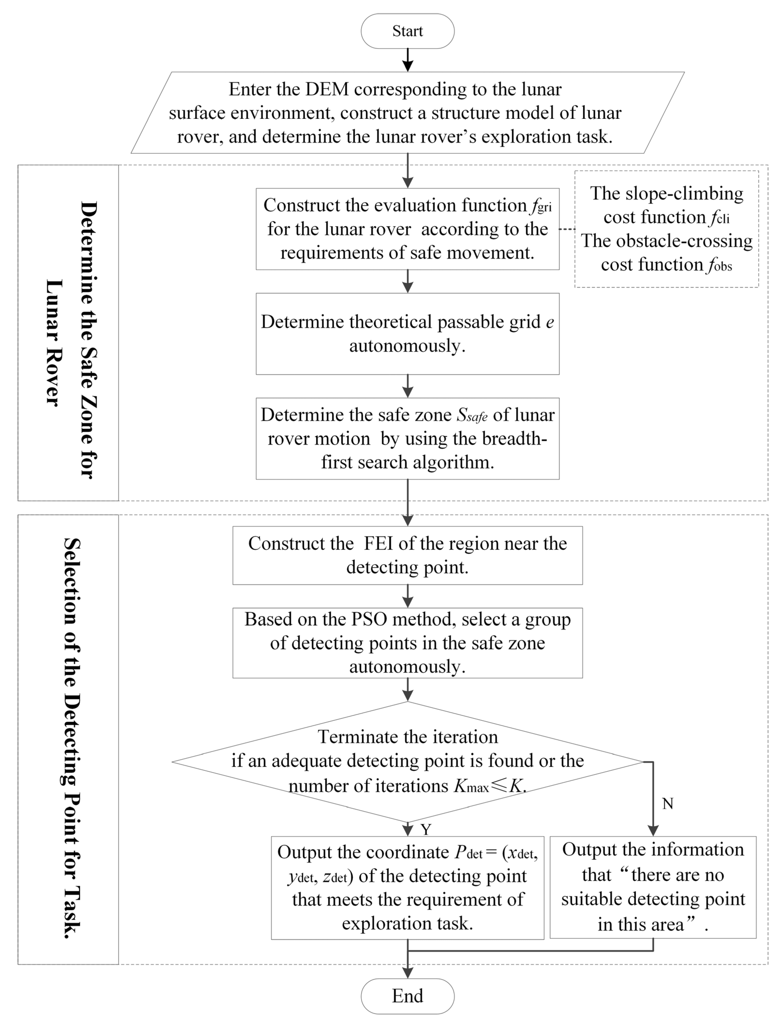
High autonomy is essential for the exploration tasks like soil sampling, rock-mineral analysis, etc., so that the rover is capable of selecting the mission-oriented detecting point independently. In this paper, a strategy for selecting detecting points is proposed, which includes three steps: Firstly, determine the lunar rover’s safe zone by considering the safety requirements. Then, establish an optimal indicator according to the characteristics of the detecting instruments, which is used to evaluate candidate detecting points. Lastly, a suitable point is selected autonomously within the safe zone by an optimization algorithm.
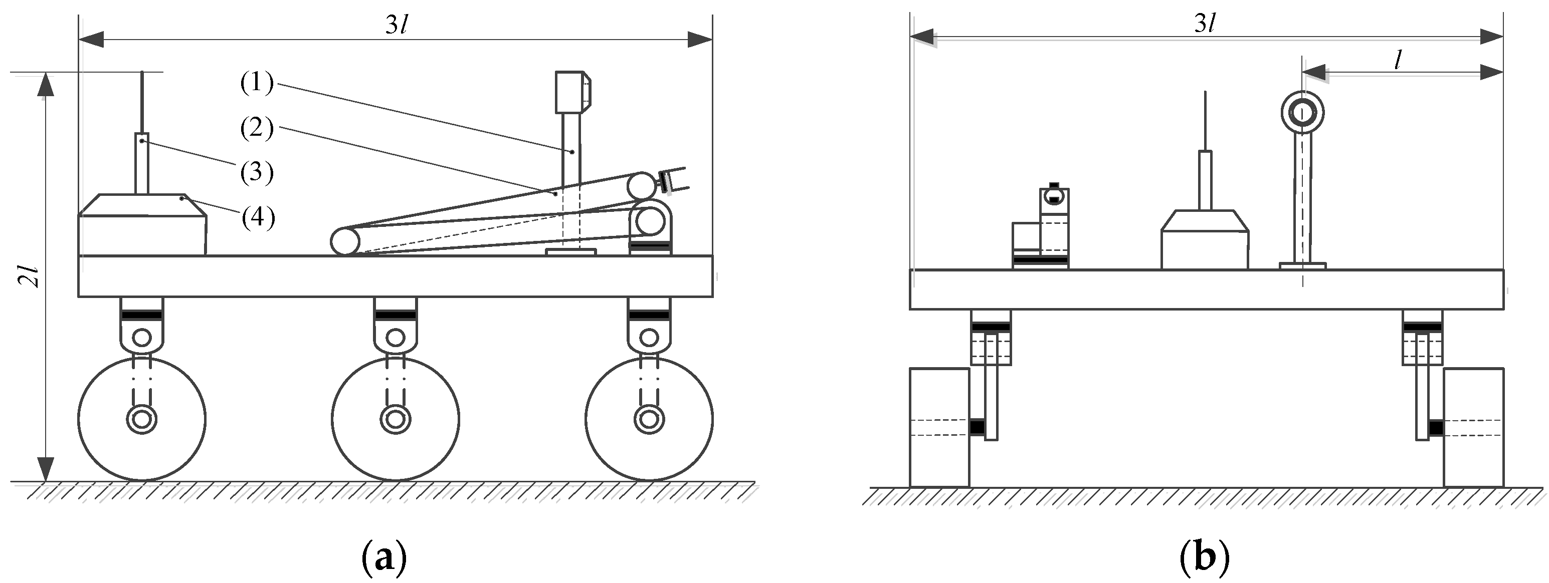
To simplify the description, a general model of the lunar rover is designed by reference to the structure of lunar rovers, the United States “Chariot”, and the Chinese “Yutu”. It is 3
l meters long, 3
l meters wide, 2
l meters high, and
M kilograms in weight (see
Figure 1). In addition, the key symbols and abbreviations involved in this chapter are listed in
Table 1:
2.1. Solution of the Safe Zone
When the rover travels on the lunar surface, the slope and obstacles (i.e., rocks and soil pits) would cause more energy consumption or even rollovers. To ensure the rover’s driving safety as well as avoid consuming excessive energy, we determine its safe zone by integrating the slope-climbing cost and the obstacle-crossing cost.
2.1.1. The Slope-Climbing Cost Function
Generally, the DEM of the lunar surface is provided by the satellites and the camera on the rover. It is represented by
N elevation points containing 3D position information, and can be expressed as a 3D array:
where
is the position vector of the
-th elevation point,
is the total number of elevation points, and
relates to the modeling accuracy of the DEM.
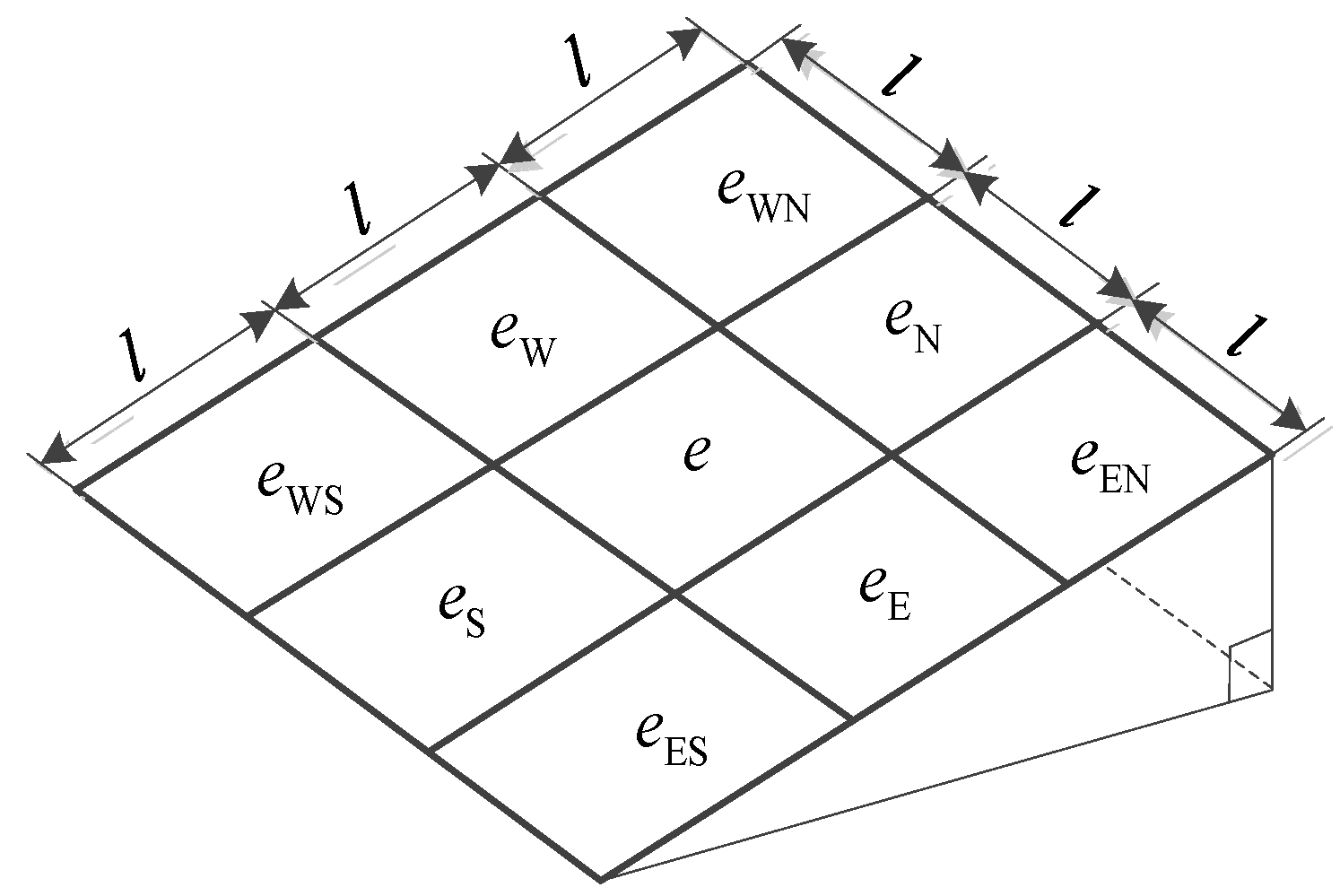
We mesh the DEM into grids, where the size of each grid is
. Thus, according to the rover’s physical structure (see
Figure 2), the region
is
.
Then we apply the least square method [
24] to fit the plane
, using all elevation point
in region
(where
is the total number of elevation points in
). That is to minimize
in the following plane equation:
where,
A,
B,
C are undetermined coefficients which can be obtained by solving Equation (3).
The spatial position of
related to the datum plane
is shown in
Figure 3.
In
Figure 3,
is the included angle between
and
;
and
have the coordinates
and
, respectively;
is the height difference between
and
;
is the distance between
and
projected to
;
and
can be expressed as follows:
Thus, the angle
measuring the slope of grid
e can be obtained by:
The structure of the lunar rover determines that it is difficult to grip the lunar surface well. When the slope angle of the grid e is too large, the rover may overturn. Therefore, the range of should be constrained to guarantee the rover’s safety, which is set as .
Since the energy consumption can affect the sustainable operation (i.e., service life) of the lunar rover, we use it to evaluate the traversability of a grid. According to the requirement of sustainable operation, the slope-climbing cost function of the lunar rover is defined as
where
is the gravitational acceleration on the lunar surface. Using Equation (6), the energy consumption for overcoming gravity can be evaluated when the rover passes a grid.
2.1.2. Obstacle-Crossing Cost Function
In the process of fitting plane macroscopically, some small obstacles are eliminated, such as small rocks, small soil pits, etc. The energy cost to cross them cannot be ignored in real missions, but is not included in . Therefore, an obstacle-crossing cost function needs to be considered in the mission analysis.
In this section, we construct the obstacle-crossing cost function based on the energy consumption to cross the maximum obstacle, which is characterized by the extreme height of each elevation point relative to in the grid e.
The distance
of any elevation point
in
moving along the normal direction to the plane
can be obtained by
By combining the distances
corresponding to all elevation points, a set
is obtained. The maximum height
of the obstacles in the plane can be given by
where
and
are the maximal and the minimal in set
, respectively.
The highest obstacle that can be crossed is defined as
, which is related to the rover’s structure. If the obstacle’s height
is greater than the maximum surmountable obstacle height
, the lunar rover cannot pass through grid
e. A safe pass can only occur when
. The obstacle-crossing cost function of the lunar rover can be expressed as:
2.1.3. Solution of the Safe Zone
Based on the slope-climbing cost function and the obstacle-crossing cost function, an evaluation function
can be constructed, which represents the cost of crossing a grid, given by
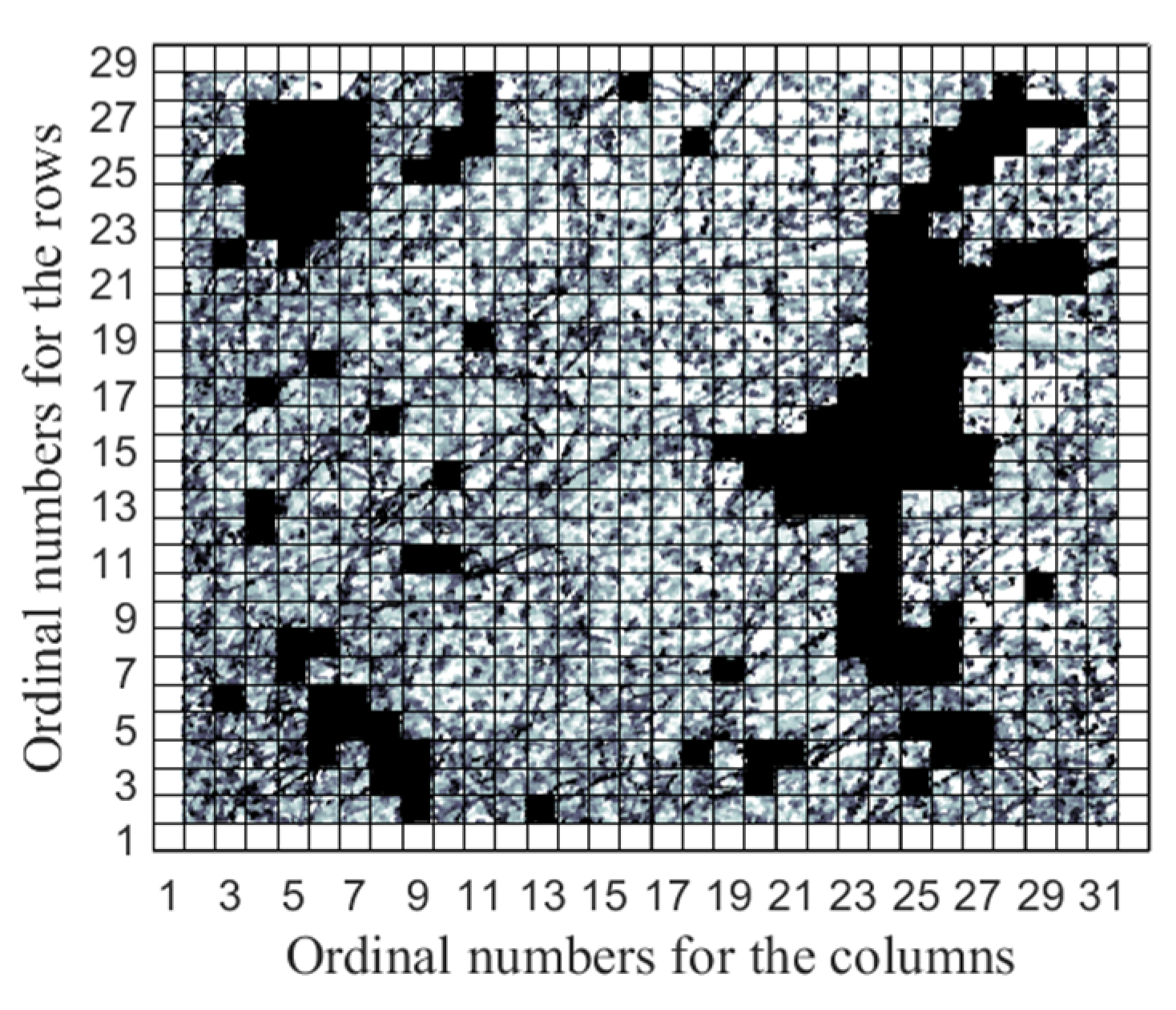
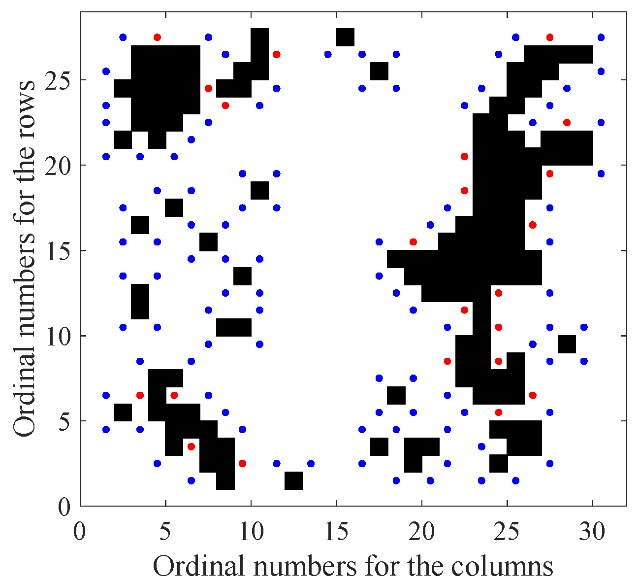
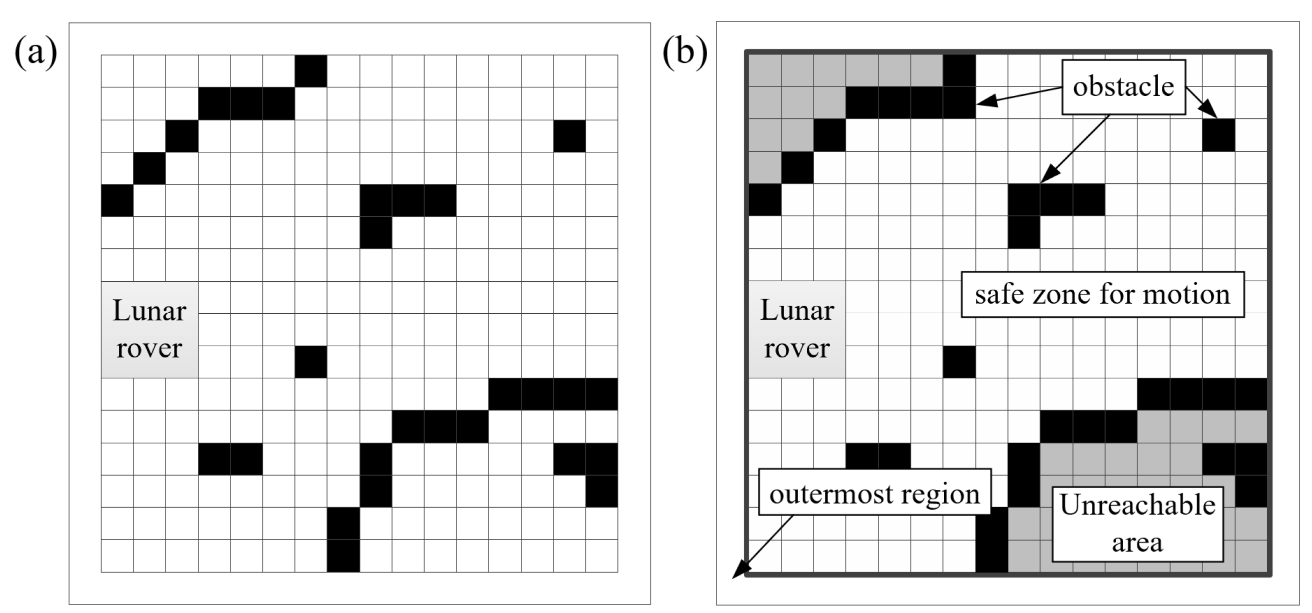
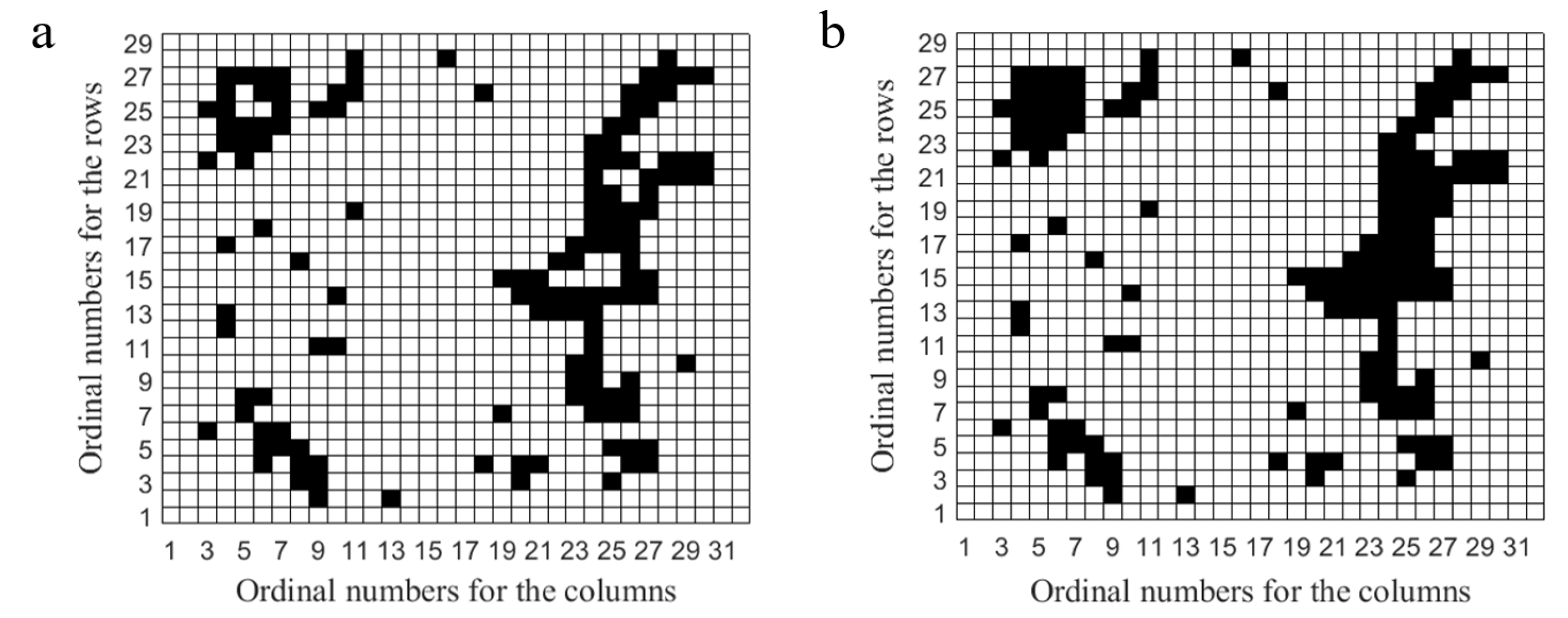
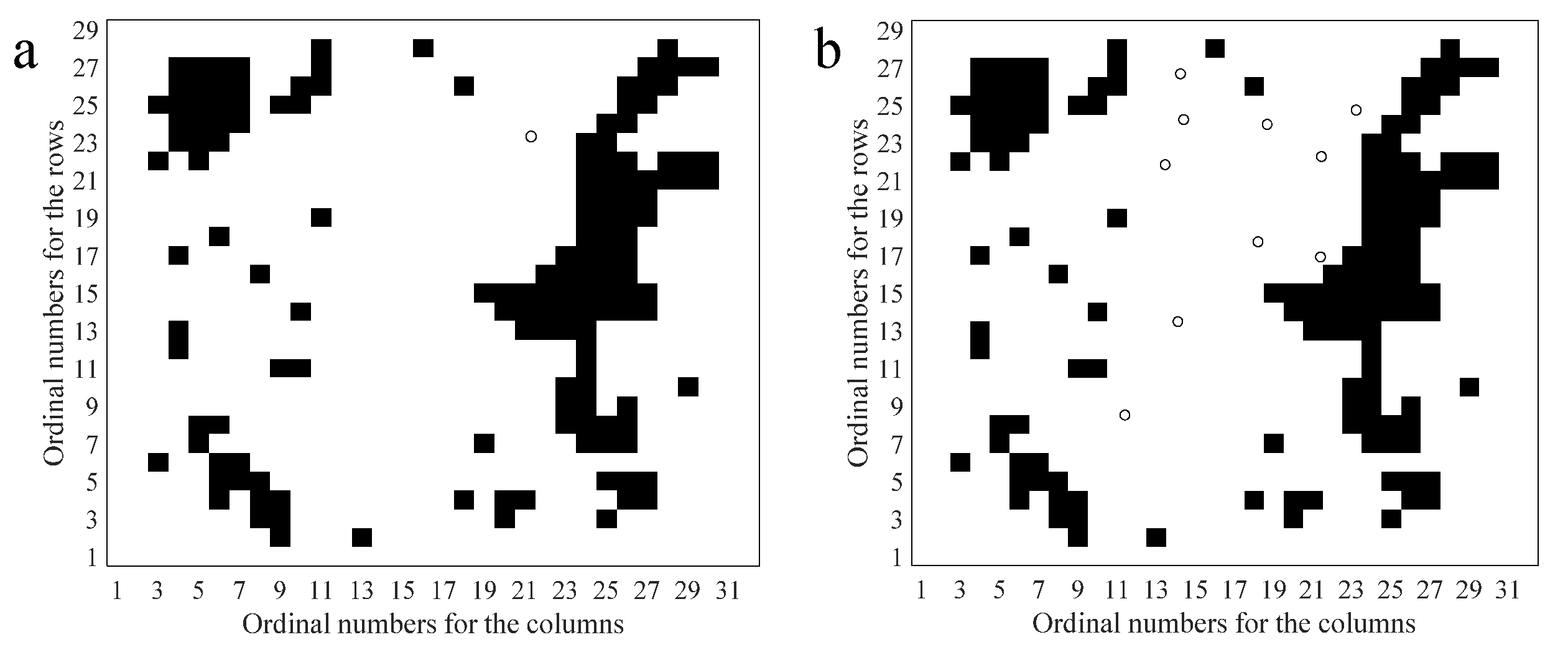
According to Equation (10), whether a specific grid is passable by the rover can be determined. For example, the black grids in
Figure 4a are not passable, where the value
is calculated as
. On the contrary, white grids are passable where
is not infinite values. However, some white grids only determined by Equation (10) are still unreachable for the rover because they are obstructed by their surrounding black grids. We call them unreachable areas—grey regions in
Figure 4b.
To obtain the safe zone, we introduce the seed-filling method to exclude the unreachable area from all the white grids calculated by Equation (10). Specifically, the location of the lunar rover is chosen as the seed; then, we apply the breadth-first search algorithm [
25], one of the common methods to find the largest connected domain, to search the grids adjacent to the seed. Grids with the same property are merged into one set, and the safe zone can be determined. Note that, due to the structural constraints of the lunar rover, the passing cost of the outermost region (see
Figure 4b) cannot be calculated since it is not considered a safe zone.
At this point, the autonomous solution of the safe zone has been obtained.
2.2. The Selection Strategy of the Detecting Point
In this section, we propose an automatic strategy to select the mission-oriented detecting point for the rover. In general, a flat detecting region is beneficial to the detecting instruments. Therefore, we introduce the FEI to evaluate the flatness of a detecting region, and then we use the particle swarm optimization (PSO) algorithm to search for a flat region as the candidate detecting point.
2.2.1. The FEI
For missions like lunar soil sampling and rock mineral analysis, the X-ray mass spectrometer is the main equipment, and two necessary conditions should be met for the normal operation [
26]:
Detecting orientation. When the X-ray mass spectrometer analyzes soil on the Moon surface, it needs to receive the reflected light of the X-ray emitted by itself. Therefore, its axis should coincide with the normal to the fitted plane corresponding to the detecting point.
Detecting distance. The distance between the mirror surface of the X-ray mass spectrometer and the detecting point should be smaller than the maximum exploration range. However, some features of the detecting region, such as convex and concave, may lead to volatility in distance. To meet the distance requirement, the detecting point should have high flatness.
The required detecting orientation can be achieved by adjusting the pose of the vehicle-mounted end effector, on which the X-ray mass spectrometer is installed. Therefore, this paper merely focuses on the detecting distance requirement.
The flatness of a region can be measured based on the DEM because it includes detailed topographic information. The standard deviation is a measure of the fluctuation in height of elevation points, and that of a flat region is usually small. Thus, the standard deviation is taken as the FEI to estimate the flatness.
Assume that point
is one of the candidate detecting points, then the detecting region is the circular region with a radius
at
, where
is determined by the mirror radius of the X-ray mass spectrometer. This region contains
elevation points, which make up the set
(see
Figure 5).
The
elevation points are used to fit the plane
as stated in
Section 2.1.1, and the distance
from the points
in the set
to
is calculated by Equation (7). The FEI
is defined by the standard deviation of
where,
is the mean of all the distances
.
2.2.2. Selection of the Detecting Point
A suitable detecting point should be selected in the region which meets the condition of detecting distance in the safe zone. For a large scale of the lunar environment, in which the safe zone is usually in several thousand square meters, it requires a heavy lift in time and resources for manual work. To overcome those shortcomings, the PSO is applied to select the detecting point autonomously in this paper, which stands out with fast convergence and high precision [
27].
Randomly select
elevation points in the safe zone, denoted as
.
can be determined according to the size of the safe zone. The first two dimensions
of the set
are extracted to initialize the particle swarm. The fitness function
of the particle is constructed according to the FEI which is shown as Equation (12):
where the value range of
is
;
is an amplification factor. The high value of
means that the area where the elevation points of particles are located is relatively flat.
According to the requirements of the flatness of the detecting point, the fitness threshold of the particle can be set, and the fitness of the final optimum particle needs to be greater than or equal to . The upper limit of the iteration is set according to the requirement of calculation efficiency.
So far, the best mission-oriented detecting point can be selected. The entire process of the detecting point selection strategy is shown in
Figure 6.
3. The Sampling-Based Path Planning Method under Linear Guidance (The Integrated Sampling-Based and Linear-Guided Path Planning Method)
Sampling-based global path planning algorithms such as PRM and visibility graph method are efficient in path planning in a static working environment [
28]. These algorithms firstly construct roadmaps, then search the path quickly with the roadmaps to obtain feasible paths. However, many sampling points and connecting paths fall in open areas far from obstacles. These points have no obvious effect on improving the connectivity of the roadmap.
In this section, a sampling-based path planning under the linear guidance method is proposed, taking advantage of the higher efficiency of the linear path planning in open areas. It includes three steps: First, divide the safe zone into open areas and dense obstacle areas, and the dense obstacle areas are sampled to construct local roadmaps. Second, the initial path is constructed based on the linear path planning, which is then modified and simplified to avoid colliding with obstacles according to the sampled local roadmaps. Finally, the original map and several supplemented maps for new tasks are combined by the map extension strategy, which fully utilizes the local roadmap to improve the efficiency of roadmap reconstruction.
3.1. Sampling in Areas with Dense Obstacles
3.1.1. Division of the Safe Zone
To divide the safe zone clearly, the area within ( is determined by the grid size) around the obstacle is defined as the dense obstacle area. The detailed division process of the open area and the dense obstacle area is introduced as follows:
In a workplace
containing obstacles, the center of grid
is denoted as
. Take
as the center (see
Figure 7) and search for the nearest obstacle grid as follows:
First, search all grids in the n-th layer that encloses . The maximum number of the layer ( indicates an upward rounding).
During the search of grids in each layer, the four grids in the horizontal and vertical directions are searched preferentially, and are shown as
in
Figure 7. If neither of the searched grids is the obstacle grid, the upward and downward adjacent grids of
and
are searched, respectively. Similarly, the left and right adjacent grids of
and
are searched, respectively.
The first obstacle grid detected is the nearest obstacle grid, for example, the dark red grid centred at point B in
Figure 7. The distance
can be calculated between the nearest obstacle grid’s center
and
:
If no obstacle grid is detected by the end of the search, the grid does not belong to the dense obstacle area, and then is set as .
According to the value of
, the dense obstacle area and the open area can be expressed as a set, given by
3.1.2. Sampling Points in the Areas with Dense Obstacles
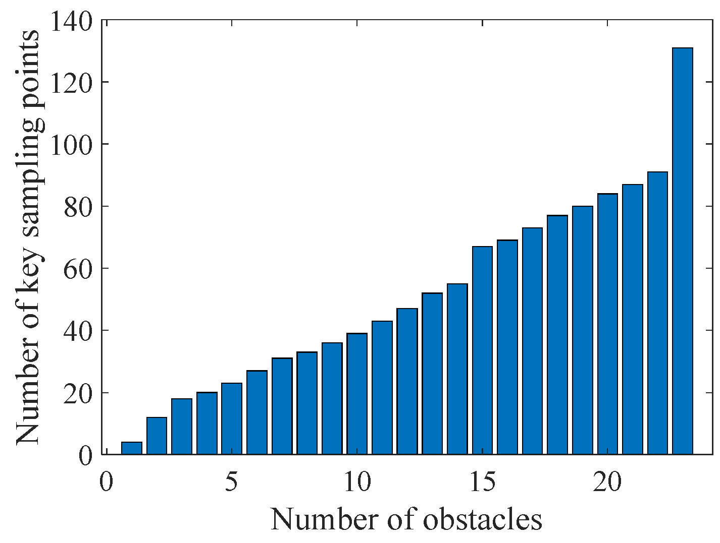
The number and distribution of the sampling points directly affect the efficiency of path planning and the connectivity of the roadmap. A large number and a worse distribution can increase not only the complexity of the search problem, but also the computation time. However, fewer sampling points, although costing less computational time, might fail concerning a feasible path. If each sampling point includes rich information of obstacles, the total number of sampling points can be reduced. In this paper, the shape points and the distance points are used to characterize the contour features of the obstacles.
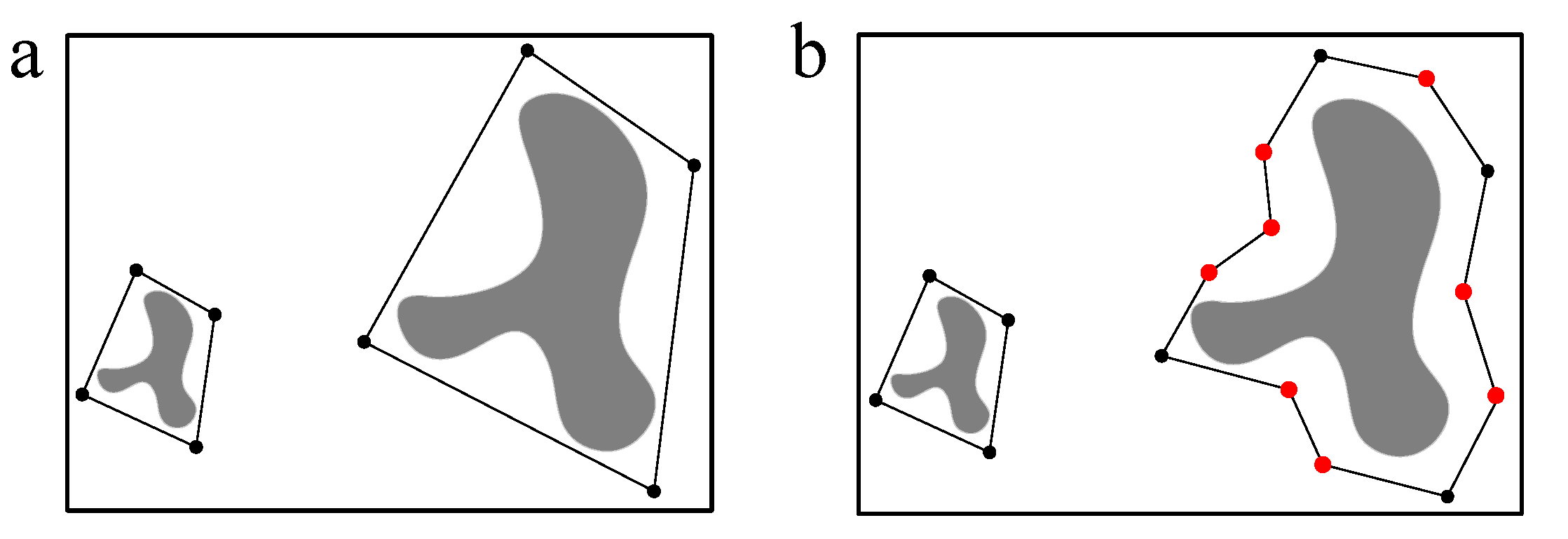
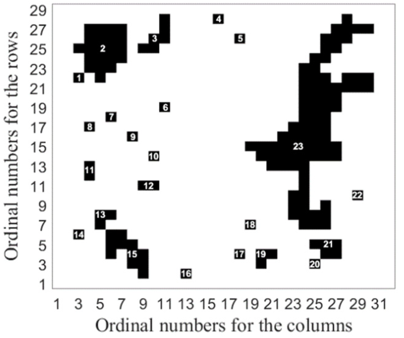
For the obstacles with the same size, the complexity of the shape determines the number of shape points. Prominent parts of the obstacle depict the effective contour of the obstacle and contain rich connectivity information. As shown in
Figure 8a, parts surrounded by dashed lines can improve the connectivity of the roadmap. Considering the geometric feature, we sample points in the prominent part of obstacles, which can be represented by partial grids (see the orange grids in
Figure 8b).
According to
Section 3.1.1, a grid
in the dense obstacle area can be ensured, whose center locates on the diagonal of the nearest obstacle grid
B. The distance between the center of
and that of
B satisfies the following relationship
The center of the grid
is chosen as the shape point because it can represent the bulged part of the obstacle to some extent. The above process corresponds to the line 03~08 in Algorithm 1. We define the set of shape points as follows:
The number and distribution of shape points are the same for obstacles with similar shapes but different areas. As the area increases, the distance between shape points increases, and the connected paths in the roadmap are lengthened, as shown in
Figure 9a.
However, in the long narrow channels, the shape points do not enhance the connectivity of the roadmap significantly. To solve this problem, distance points are introduced in the paper; see the red points in
Figure 9b. The set composed of the distance points
is denoted as
, on which the following constraints are imposed:
;
for ;
for and .
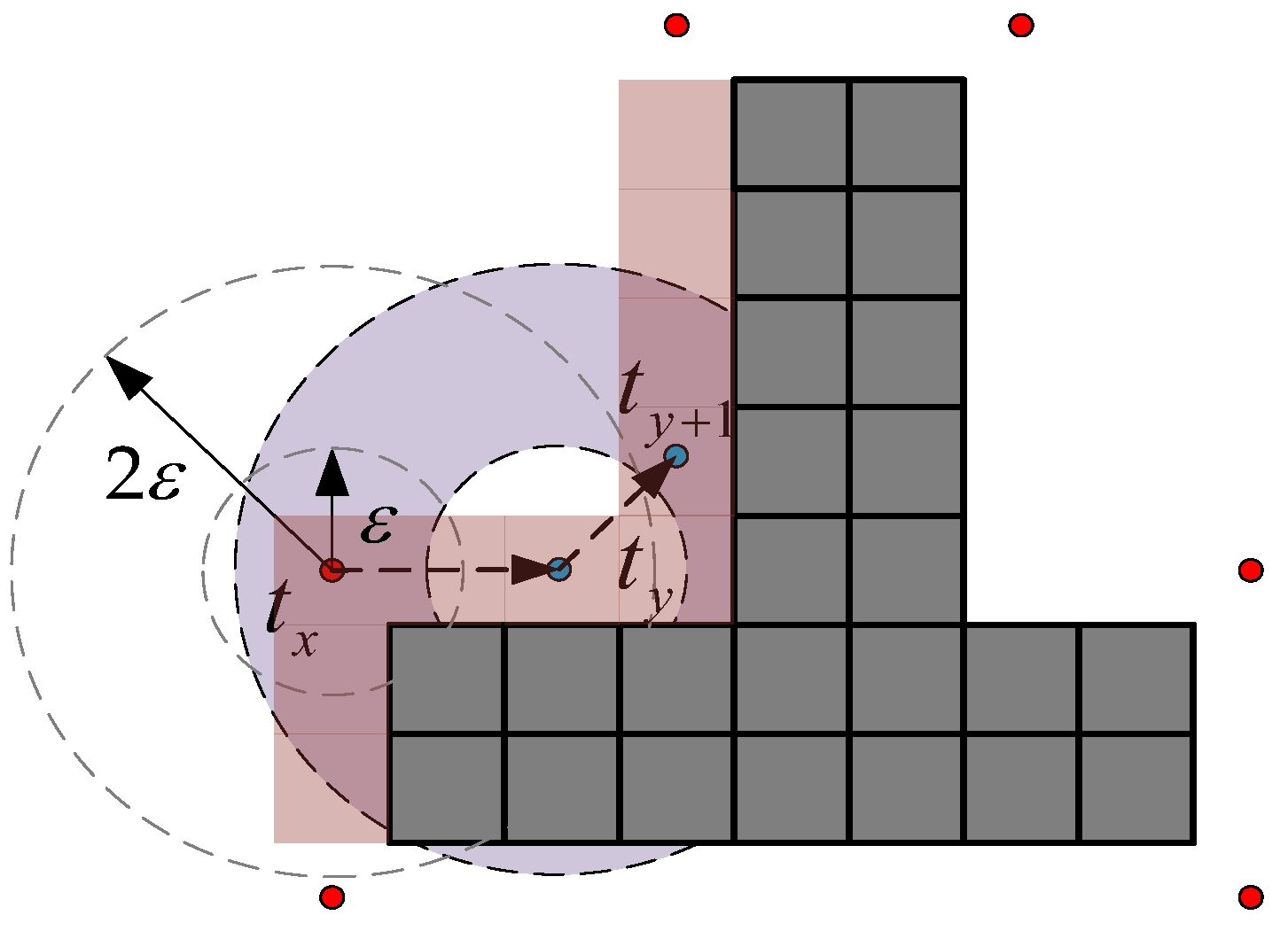
To meet the above three conditions simultaneously, the distance points are selected by traversing all the elements in as follows (the lines 09~15 in Algorithm 1):
- (1)
Determine the annular area with radius
and center
(see
Figure 10).
- (2)
Search the center of grid in the overlap between the annular area and the dense obstacle area. If no center point is detected within the overlap, turn to (1).
- (3)
Calculate the Euclidean distance
between
and
. Notice that
may not be unique, in which corresponding to the minimum distance
is taken as a distance point
as follows
Then, put the point into the set .
- (4)
Take as the center of the annular area with radius ; turn to (2).
| Algorithm 1: Sampling Points |
| 01 | Require: Initialize , , , is the side length of grid, is the threshold of the area with dense obstacles. |
| 02 | if do |
| 03 | for each the center of the grid |
| 04 | find out the nearest obstacle grid to |
| 05 | if |
| 06 | |
| 07 | end |
| 08 | end |
| 09 | for each |
| 10 | for each |
| 11 | if do |
| 12 | |
| 13 | end |
| 14 | end |
| 15 | end |
| 16 | end |
Based on the obtained sampling points, the local roadmap can be constructed. All the sampling points in a circle with centre and radius r (r can be determined according to the connecting requirements of the roadmap for path planning) are connected to the point () to get edges. The edges which do not collide with obstacles are stored to the set E. The roadmap is made up of the set of sampling points and the set of collision-free edges E. By constructing a roadmap, the path planning in continuous space can be solved in the topological space; thus, the search complexity of path planning is reduced.
3.2. Path Planning under Linear Guidance
There is no connecting path in the open area since all the sampling points are located in the dense obstacle area, and the connecting paths of the roadmap are distributed around the obstacle. This section adopts a linear path in the open area as the path guidance.
3.2.1. Planning the Linear Path
Considering the generality, we assume that there are some arbitrary obstacles in the map and specify the rover’s current location and detecting point. It starts by establishing a linear path between the two points:
where,
is the coordinates of the current location and
is the coordinates of the detecting point.
If no obstacle intersects with the linear path, this linear path is the final path, as
in
Figure 11. Otherwise, it is necessary to find out the feasible paths that can bypass obstacles. The intersecting points with the edge of obstacles are denoted as
(see
Figure 11).
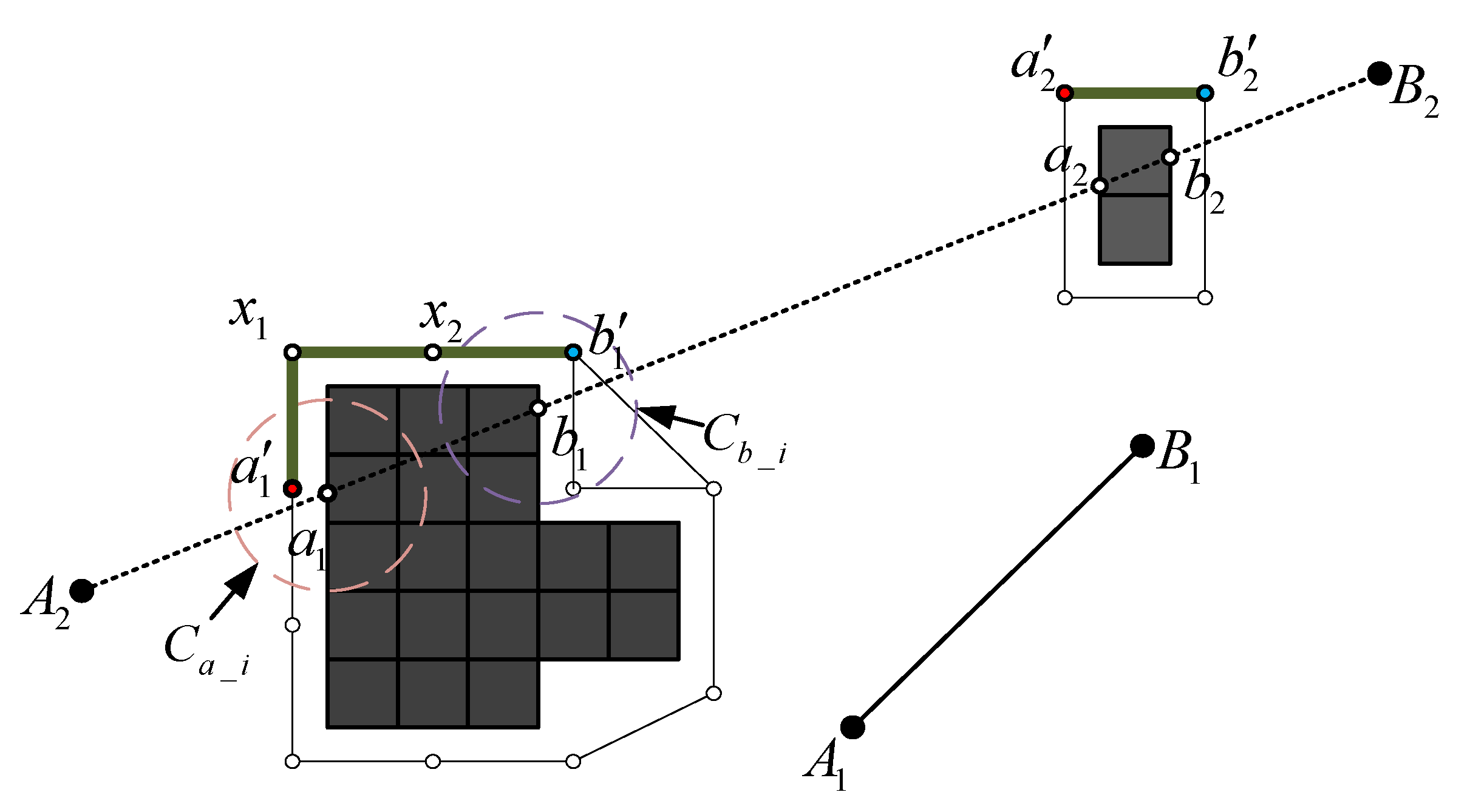
3.2.2. Searching for Local Feasible Paths in the Roadmap of Dense Obstacle Areas
If the linear path intersects with obstacles, the A* heuristic search algorithm is adopted to search the local feasible path in the roadmap
constructed in
Section 3.1. The local feasible path can help to bypass the obstacle. The sampling points nearest to
and
are used as the starting and the ending point to search the path. The maximum distance between each sampling point and the obstacle is strictly required to be
in
Section 3.1; there must be one or two sampling points
that meet
. Therefore, the search range for the nearest sampling point of
, which is denoted as
, is the circle with center
and radius
. The nearest sampling point searched as
is recorded, and so is
. The local feasible path is
(see
Figure 12), and this process corresponds to line 07~22 in Algorithm 2.
3.2.3. Solution of the Best Feasible Path
An obstacle-free path can be obtained by modifying the linear path with local feasible paths. However, it is rather tortuous. In the paper, a forward trial method is used to enhance the obstacle-free path by linearizing it.
Take for example to explain this method.
Step1: Take as the starting point; connect with the next node . Try to connect with ; if does not intersect with any obstacle, is discarded, and so on. Get the first furthest point and the first valid shortcut .
Step2: Take as the new starting point; then repeat Step 1. Get the second furthest key point and the second valid shortcut .
Step3: Take as the new starting point; then repeat Step 1. Get the third valid shortcut .
So far, the final feasible path
has fewer turn points and is the best possible shortcut obtained (see
Figure 13), and this process corresponds to line 24~34 in Algorithm 2.
| Algorithm 2: Path Planning Strategy under Linear Guidance |
| 01 | Require: Specify the current location of the rover and the detecting point . |
| 02 | Initialize the roadmap , the obstacle areas , the area with dense obstacles , the set of the key points . |
| 03 | Initialize the finite set of the points of local path and the set . |
| 04 | Plan a linear path from to . |
| 05 | Find intersection points of the straight line and the : |
| 06 | |
| 07 | if is not NULL do |
| 08 | for to |
| 09 | Take all elements of in the search range as the set . |
| 10 | for each element of |
| 11 | Calculate the distance between and . |
| 12 | end |
| 13 | if correspond to the minimum of |
| 14 | |
| 15 | end |
| 16 | Take all elements of in the search range as the set , and the same process as . |
| 17 | Search the path from to in by using A* algorithm. |
| 18 | for each node of the |
| 19 | |
| 20 | end |
| 21 | end |
| 22 | end |
| 23 | |
| 24 | for to length |
| 25 | for length |
| 26 | |
| 27 | |
| 28 | if the straight path intersects with obstacle do |
| 29 | |
| 30 | |
| 31 | end |
| 32 | end |
| 33 | end |
| 34 | |
3.3. Map Extension
With the deeper exploration of the lunar rover, the explorable area continues to expand. The detection of a new area or the change of a local area can render the existing roadmap unusable, so that the roadmap needs to be updated. Reconstructing a large-scale and complete roadmap of the lunar environment would take a long time, which would lead to a sharp decrease in planning efficiency. To improve the efficiency, map extension is carried out combined with the roadmap’s local feature.
3.3.1. Data Processing of Map Extension
The following process needs to be done to execute the map extension:
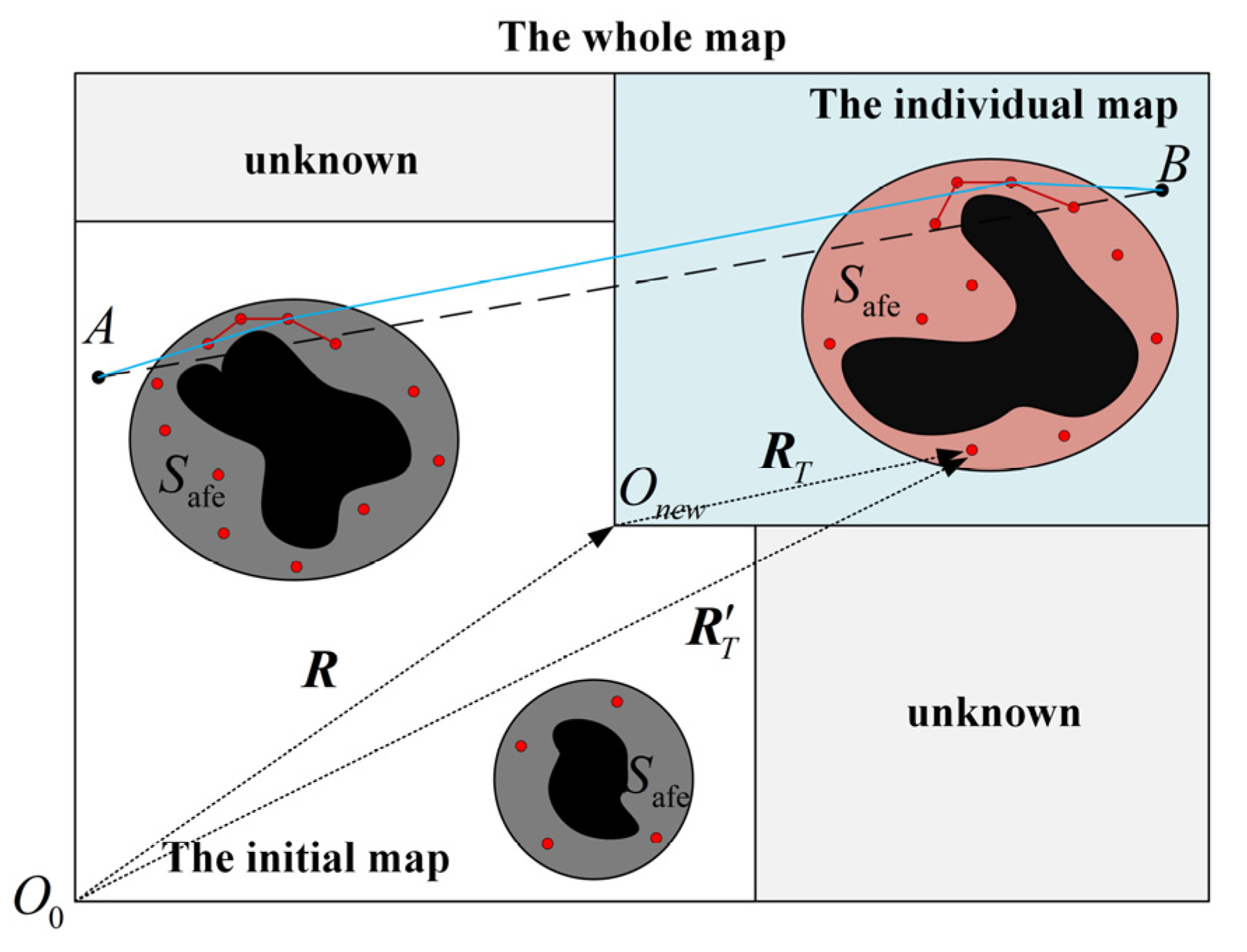
Map preprocessing. The whole map is the same as the initial map at the beginning.
Roadmap construction. According to Equation (10), the initial safe zone for motion is determined. The set of sampling points
is got and the roadmap
is constructed by
Section 3.1.
Set collections and , the sampling points set and the roadmap of the initial map or the individual map, respectively.
The part that needs to be updated is treated as an individual map, and the safe zone
, the sampling points set
, and the roadmap
of it are obtained according to
Section 2.1 and
Section 3.1. According to the relative position
between the individual map coordinate origin and the whole map origin, the coordinates of each point are updated. For example, if the position of the key point in the individual map is
, then its position
in the whole map can be updated as follows:
Store the updated sampling points set , the roadmap in and , respectively.
The process of path planning for the extended map is the same as that for the initial map:
Plan the initial path with a linear line in the whole map.
Once the initial path intersects with the obstacles, search for a local feasible path using the A* algorithm in the roadmap to bypass the obstacle. Note that, if the obstacle locates in the individual map, the local feasible path will be searched in the roadmap corresponding to the individual map.
Use the forward trial method to get the final feasible path.
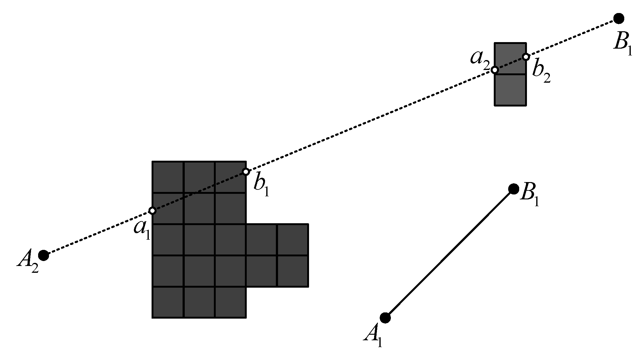
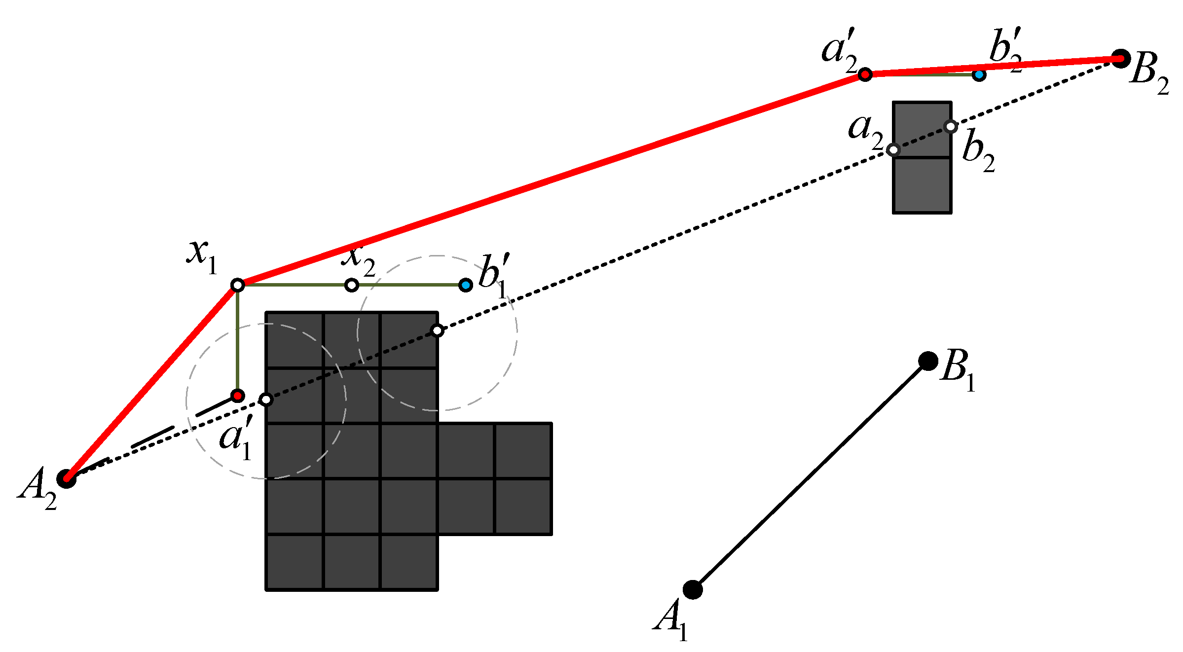
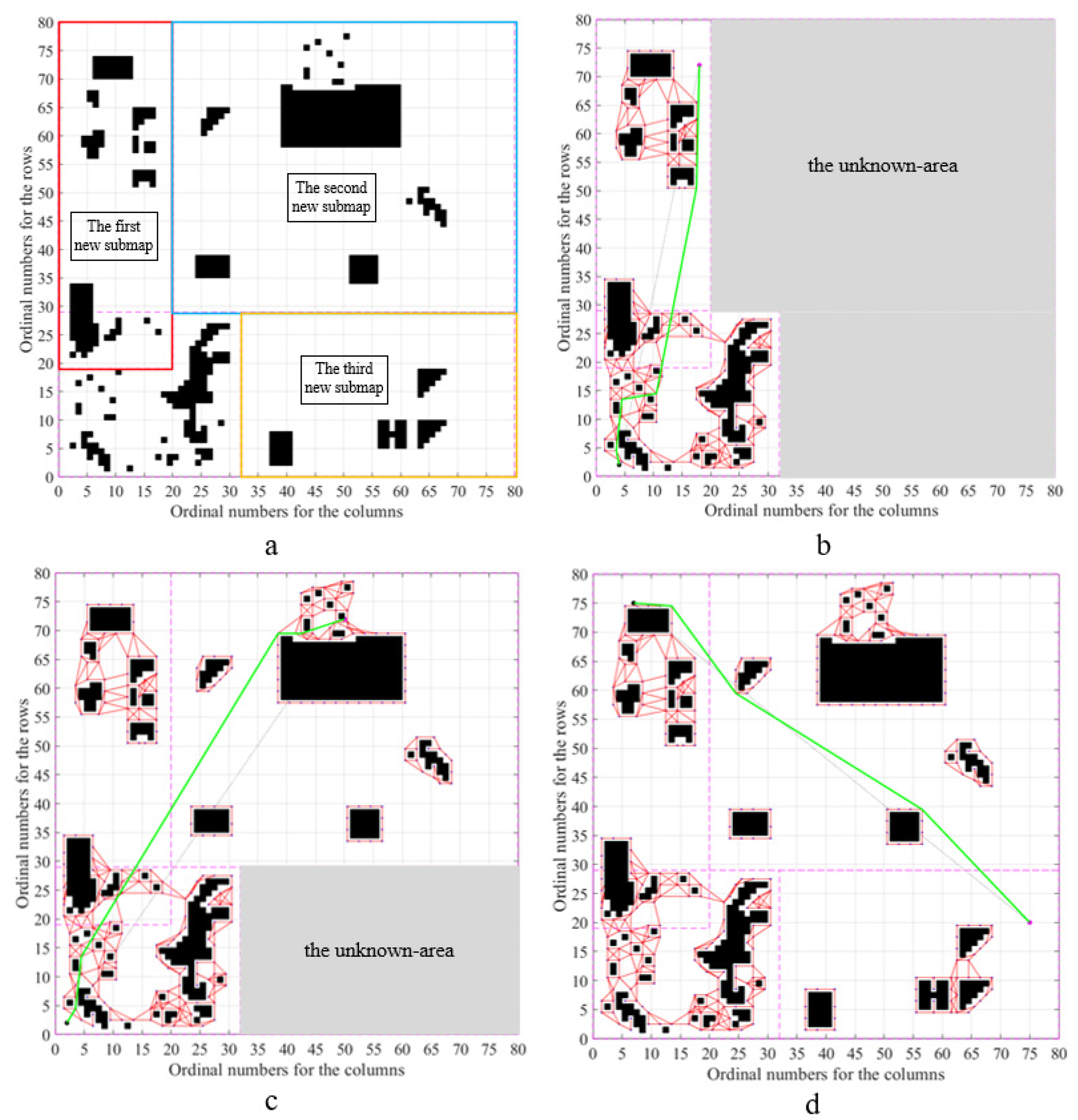
For example, the initial path is planned from point
to point
as shown in
Figure 14, and it intersects with two obstacles. One is in the individual map and the other is in the initial map. The local feasible paths are searched in the roadmap, respectively, as red lines, and the final feasible path is obtained as blue lines.
Assuming that there are maps of size without overlapping each other, and they can form a whole map of size . The time complexity is by using the A* algorithm to search a local path in the roadmap of size , which is constructed from the whole map directly. Taking one of the maps as an initial map and the rest of them as individual maps, the time complexity is with the map extension. As the search scope is narrowed with map extension to some extent, the map extension strategy can improve the planning efficiency further by integrating the individual map with the initial map.
3.3.2. Path Planning with Map Extension
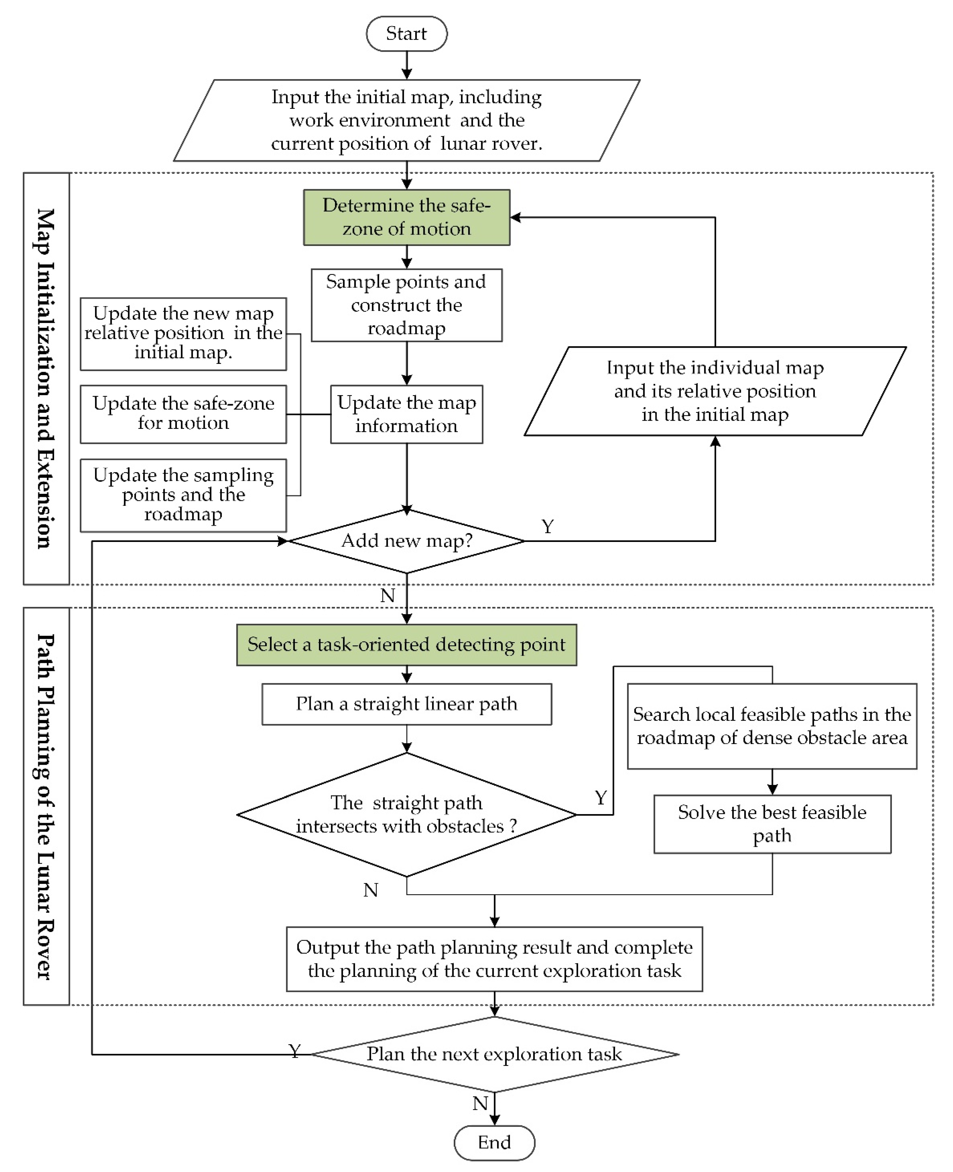
The process of path planning with map extension is shown in
Figure 15:
Step 1: Input the initial map and the initial location of the lunar rover.
Step 2: Determine the safe zone based on the slope-climbing cost function Equation (6) and obstacle-crossing cost function Equation (9).
Step 3: Sample the sampling points
and construct the roadmap
according to the strategy proposed in
Section 3.1.
Step 4: If , , are extracted from the initial map, will be used to initialize the safe zone of the whole map, and two collections and are constructed to store and . Otherwise, , , will be appended to , , after being updated according to the relative position of the individual map in the whole map.
Step5: Determine whether to add a new individual map. If required, input the new individual map and the relative position in the whole map, then turn to step 2. Otherwise, turn to step 6.
Step 6: Select the detecting point
in the safe zone
of the whole map based on the strategy of the selection of detecting point proposed in
Section 2.2.
Step 7: Obtain the final feasible path using the sampling-based path planning method under linear guidance.
Step 8: Output the path planning result, and wait for the command of the next exploration mission. If the command is received, turn to Step 5.
Based on the above process, a path planning method with map extension can be executed.
5. Discussion
In the present study, we focused on the two steps in lunar surface exploration, detecting point selection and path planning, to improve the autonomy and efficiency for the rover in lunar exploration.
Unlike most existing manual selection or single-factor selection strategies, our autonomous selection strategy took terrain features and operating conditions of detection instruments into account. This is because the number of possible detection points is greatly limited by the mobility of the rover. In
Section 4.1, we took a numerical simulation by a 16 m × 14.5 m lunar surface map. For the 10 experiments with random initial conditions, the average consumed time and final fitness value are 12.937 s and 0.988, respectively, which represent fast planning speed as well as high quality in the selected detecting point. Therefore, this strategy is more practical concerning improving the autonomy of the rover, as well as avoiding the manual misjudgment and information transmission delay between the Moon and the Earth.
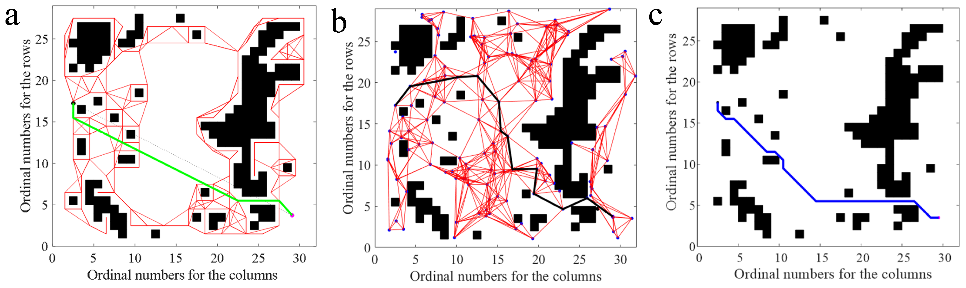
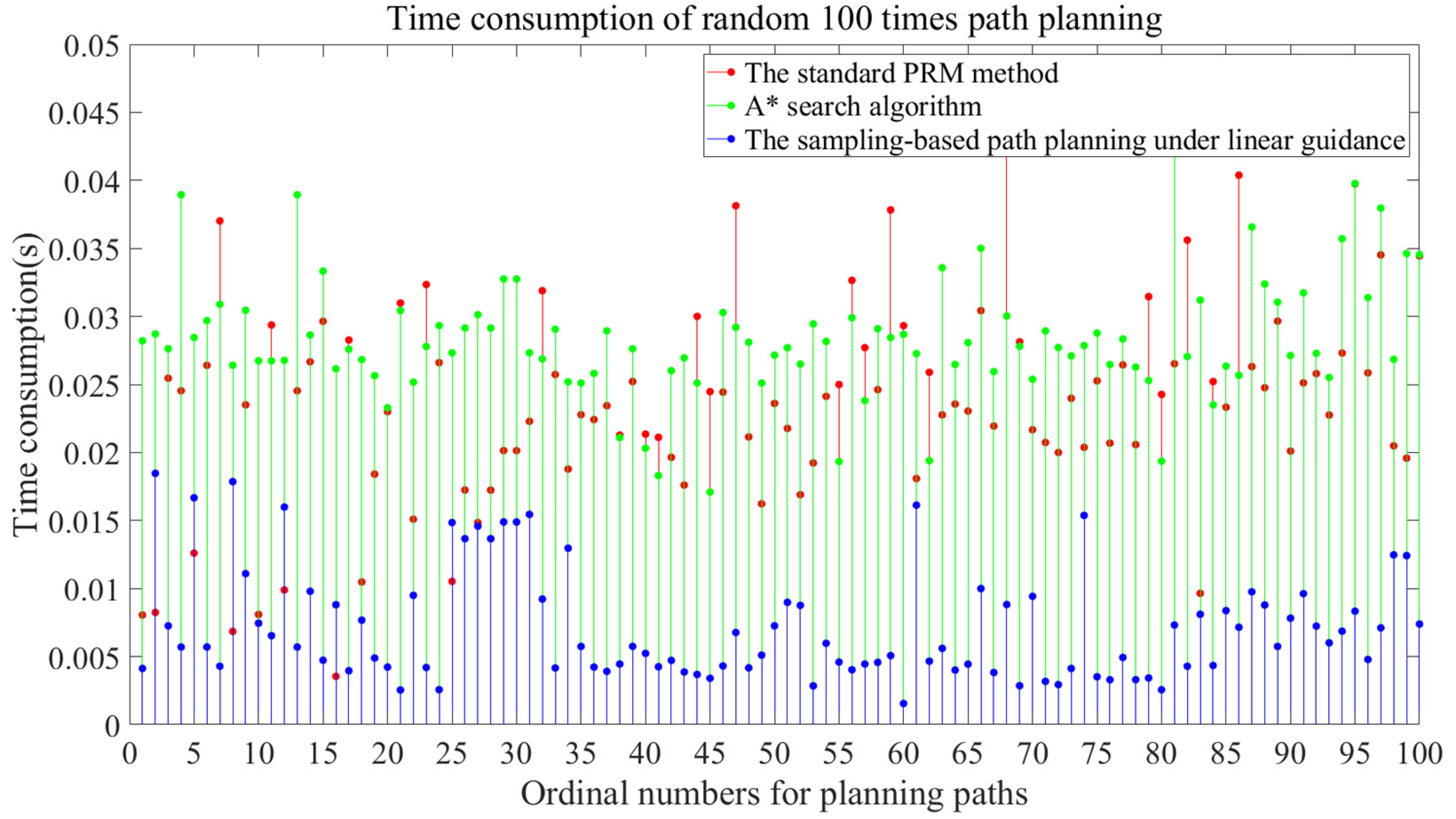
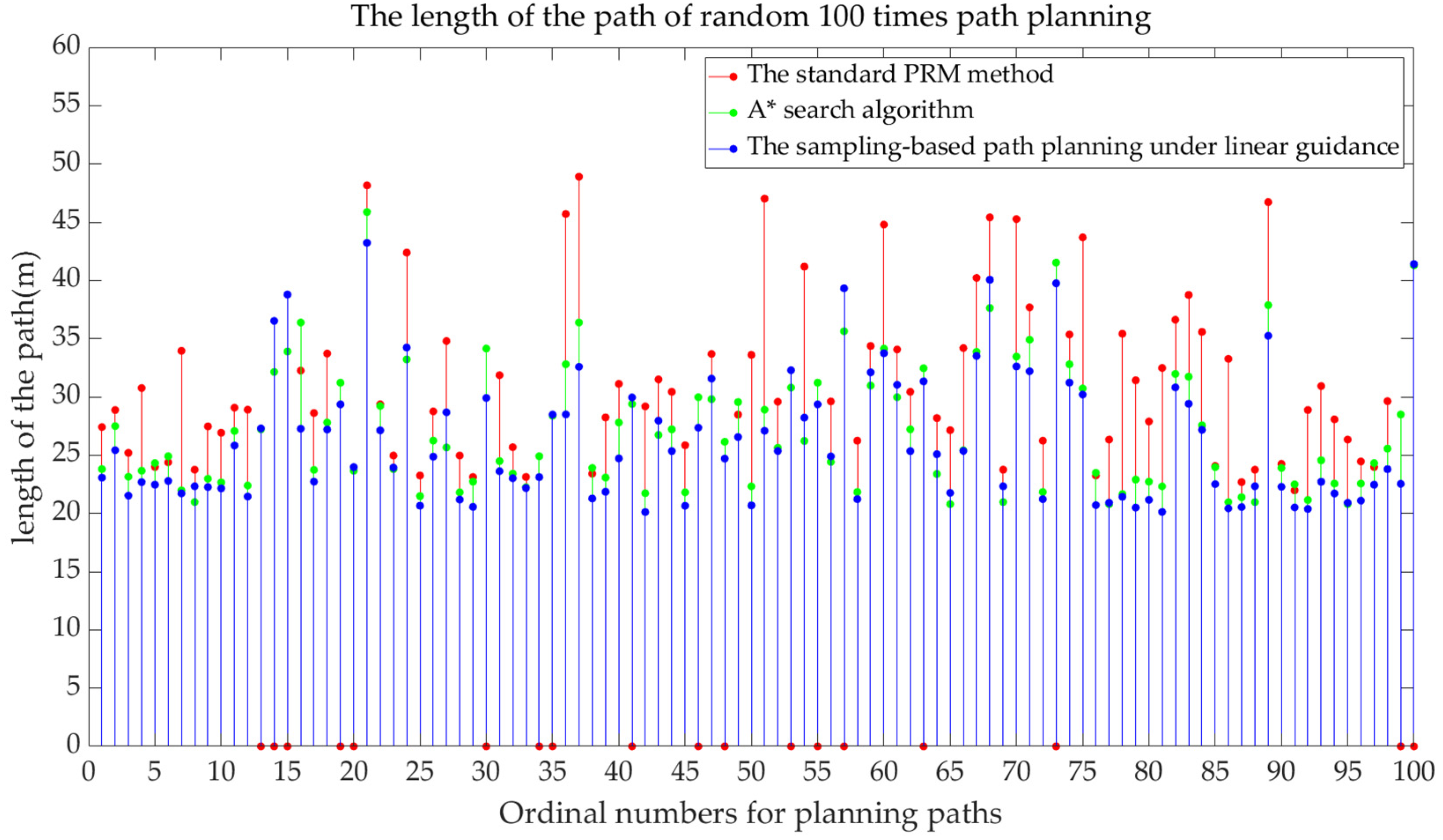
Moreover, in our proposed method, the combination of the sampling-based methods and linear guidance can make the path planning more efficient. In
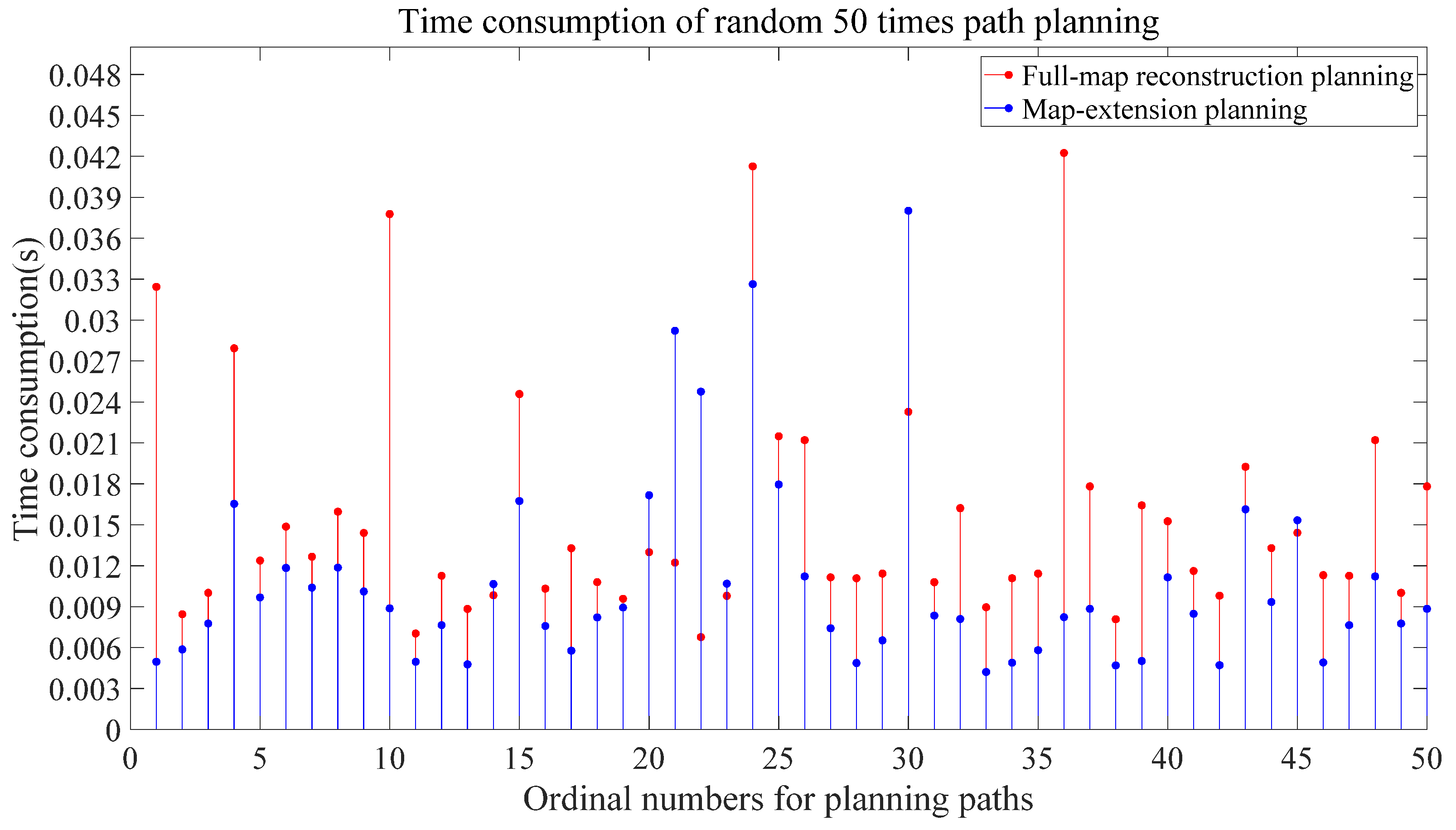
Section 4.2, an experiment as a comparison with the above lunar surface map was executed by using our method, the A* algorithm, and the PRM method. The results show that our method has great advantages in both time and quality of the path. Compared with the PRM method, the average time consumption and length of the path are reduced by 69.25% and 19.89%, respectively. That is because our method greatly improves the connectivity of dense obstacle areas, and simplifies the process of path searching in open areas. Compared with the A* algorithm, not only is the average time consumption reduced by 74.71%, but unnecessary turns of the path are also avoided. Furthermore, the map extension strategy can avoid the disadvantages of the full-map reconstruction planning in the unstructured, continually varying environment. In the simulation environment, the efficiency of roadmap reconstruction after map update has been improved by orders of magnitude, while the time for full-map reconstruction still depends on the accumulation of each reconstruction from the initial map to the current update. In addition, the time for map extension-based planning is also reduced by 31% compared with the full-map planning. This improvement is mainly due to the use of the roadmap’s local characteristics in path searching, which avoids invalid searches in the other added submaps.
Despite the great improvement in the autonomy and planning efficiency, there are still some limitations in our method. Firstly, for the map extension strategy, the special case where a common part exists between the initial map and the submap has not been considered. In this case, the submap needs to be divided to ensure that the added submap is completely new concerning the initial map. Secondly, our method is applied in a two-dimensional environment, and we hope to extend it to a three-dimensional case with appropriate improvements. These two topics will be our future concerns.


