Low-Interference Wind Tunnel Measurement Technique for Pitch Damping Coefficients at Transonic and Low Supersonic Mach Numbers ^†

Abstract

An experimental method for the determination of the pitch damping moment coefficient sum $C_{mq}+C_{m\dot{\alpha }}$ in a wind tunnel at transonic and low supersonic Mach numbers is developed. With support interference being a major issue for dynamic tests at these velocities, a minimum interference wire suspension approach is used. The motion of the wind tunnel model is restricted to a single-degree of freedom pitching oscillation through the geometry of the support system. A statistical evaluation procedure allows the simultaneous evaluation of multiple tests to increase confidence in the results. The influence of the wires as well as nonlinear effects are accounted for. The method is validated in an extensive test series at Mach numbers ranging from 0.6 to 2.0. Two reference missile models—the Basic Finner and the Army-Navy Spinner Rocket (ANSR)—are used. The results agree very well with CFD calculations throughout the transonic range. In comparison to free-flight tests the accuracy is significantly improved and result uncertainties are reduced by an order of magnitude.

1. Introduction

The pitch damping moment coefficient sum $C_{mq}+C_{m\dot{\alpha }}$ is a major factor for a projectile’s dynamic stability in flight [1]. Its knowledge early on in the design process is advantageous with regard to flight behavior and control system design. This is particularly true for flight at transonic Mach numbers where aerodynamic forces and moments can undergo significant changes for small velocity deviations.

Although CFD methods are improving, there is still a need for experimental reference data. The experimental methods most commonly used for projectile design are free-flight tests [2]. However, flight test results commonly show high scatter and large uncertainties close to Mach 1 [3]. Therefore, there is a need for an experimental method that allows for precise measurements of $C_{mq}+C_{m\dot{\alpha }}$. Various methods for its experimental determination in a wind tunnel setup have been developed [4,5], but are often not well suited for testing projectile configurations at transonic Mach numbers. The main reason for this is support interferences due to the combination of small model sizes and the larger sting support necessary for the dynamic tests, which result in large measurement uncertainties. In addition, wall interference can be a limiting factor, depending on model size and blockage ratio [6,7]. Therefore, methods like the forced-oscillation technique [8] that use a traditional sting support depend on the availability of a sufficiently large wind tunnel.

The present study aims to develop a method for the experimental determination of $C_{mq}+C_{m\dot{\alpha }}$ that is suitable for slender bodies such as missile configurations, and can be used in a wind tunnel with a limited cross-section at transonic speeds. The approach and the experimental setup, as well as the evaluation process, are described in this paper. The results are validated through comparison with CFD simulations as well as experimental and numerical data found in the literature.

Preliminary results of this project have been presented in [9].

2. Concept

The main challenges identified in relation to dynamic tests in the ISL’s trisonic wind tunnel are due to the small model size. As the tunnel cross-section is 300 $\mathrm{m}$$\mathrm{m}$× 400 $\mathrm{m}$$\mathrm{m}$, the model size is limited to diameters of up to 40 $\mathrm{m}$$\mathrm{m}$ for subsonic Mach numbers in order to limit wall interference. Most established methods for dynamic tests require some mechanical and possibly some sensor equipment either inside the model or in the model support system. In the first case, the small model size required renders the integration of such equipment challenging and thus expensive. In the second case, installing the necessary equipment inside the sting-strut support used in the ISL trisonic wind tunnel would pose the same problem and most likely increase the sting diameter, potentially causing flow blockage issues at Mach numbers close to 1.0 and driving up support interference to a level where accurate measurements are no longer possible [4,10].

The concept investigated in this project uses a wire suspension and a solid model without any internal sensors, thus enabling measurements with minimal support interference without the need for complex and expensive model instrumentation. The suspension geometry is designed such that motion limited to approximately ± 8 ${}^{\circ }$ around the pitching axis is possible. The restoring moment depends on the wire tension providing a means to control the oscillation frequency and to stabilize a statically unstable model configuration. For all other degrees of freedom the restoring forces and moments depend on the axial stiffness of the wires as a function of the Young’s modulus and the cross-section area. As this is two to three orders of magnitude higher compared to the tensioning force for the steel wires used, any significant motion is effectively blocked. The wire suspension consists of eight stainless-steel wires with a diameter of $0.5$ $\mathrm{m}$$\mathrm{m}$, which are attached to the wind tunnel side walls using a gripping mechanism. For some tests the diameter of the four front and rear wires was varied. A sketch of the wire suspension geometry is shown in Figure 1.

3. Experimental Setup

3.1. Test Facility

Tests are conducted in the transonic test section of the ISL’s blowdown-type trisonic wind tunnel. This test section is suitable for Mach numbers ranging from 0.5 to 1.5. Its rectangular test section is equipped with perforated walls to reduce wall interference by wall suction. This is enabled through a vent to the exterior atmosphere, meaning that the static pressure in the test section has to be above the atmospheric pressure to ensure proper wall suction. The maximum test duration is between 30 $\mathrm{s}$ and 120 $\mathrm{s}$, depending on the test conditions. Steady free-stream flow conditions are established within approximately three seconds after the main valve is opened.

3.2. Models

The Basic Finner [11] has been chosen as a reference model due to its relatively high pitch damping moment coefficient sum while the 7 cal. Army-Navy Spinner Rocket (ANSR) serves as a low-damping reference model. Results from free-flight tests at transonic and supersonic Mach numbers as well as from CFD investigations are available in the literature for both configurations [12,13,14,15,16]. The caliber D of both models is 20 mm. This results in a blockage ratio of 0.26% in relation to the wind tunnel cross-section. The model dimensions are shown in Figure 2.

The wires are attached to the models either through an internal gripping mechanism or an adhesive connection in a through-hole. Four central wires are situated in the yz-plane and define the model motion’s center of rotation. Ideally (but not imperatively) this coincides with the model’s center of gravity. Four additional wires are placed in the horizontal plane, pairwise at equidistant positions to the front and rear of the center of rotation. The wind tunnel setup is shown in Figure 3. A small bore to attach the release mechanism is placed on the afterbody of the model.

Models are manufactured from solid steel. In order to conduct tests at increased oscillation frequencies, an additional low-inertia Basic Finner model has been manufactured from aluminum.

3.3. Measurement Setup

The pitching motion is recorded using a high-speed camera mounted outside the wind tunnel, perpendicular to the pitching plane. An evaluation tool based on a corner-detection algorithm developed at ISL [17] is used to extract the pitch angle from the recorded images. The accuracy of the corner-following algorithm depends on the number of pixels between the tracking markers on the model, for the setups used the error in the determined pitch angle has been on the order of ± $0.01$ ${}^{\circ }$. As the model oscillation frequency varies between 10 Hz and 40 Hz in case a steel model is used, a frame rate of 1000 Hz has shown to be a reasonable compromise between accuracy and evaluation time. For the aluminum model, the oscillation frequency can rise above 60 Hz for some Mach numbers. In these cases, the frame rate has been increased to 2000 Hz to improve accuracy.

3.4. Experimental Procedure

At the start of each test run, the release mechanism is attached to the rear of the model, which is thus held at a small initial displacement angle of approximately 8 ${}^{\circ }$. Once steady free-stream flow conditions are established, the release mechanism is triggered manually and the model begins to oscillate. After the amplitude has decayed, the tunnel flow is turned off.

The influence of the wire tension force on the results was examined by modifying the stiffness of the suspension system. As the effect on the wind-on oscillation frequency was found to be small, the influence of the frequency on the stability derivative was studied using the low-inertia aluminum model.

The mechanical damping contribution, necessary for accurate measurement results as described in Section 4, has to be determined through tare runs. These were conducted directly in the wind tunnel test section at wind-off conditions. Separate tests in a vacuum tank have shown that the remaining aerodynamic damping during those tare runs is small enough to be neglected.

4. Evaluation Approach

Based on the full equations of motion a simplified single-degree of freedom equation for the pitching angle $\theta$ has been derived under the assumption of negligibly small motions in all other degrees of freedom. The simplified pitching motion is described by the differential equation:

$$\ddot{\theta }+2{\delta }_{tot}\dot{\theta }+C_1\theta +C_2{\theta }^3=0,$$

(1)

where the linear stiffness coefficient $C_1$ describes both the aerodynamic as well as the mechanical influences whereas the cubic stiffness coefficient $C_2$ describes the mechanical influence caused by the suspension geometry. The damping coefficient ${\delta }_{tot}$ is the sum of the aerodynamic and the mechanical damping coefficients ${\delta }_{aero}$ and ${\delta }_{mech}$. While ${\delta }_{aero}$ can be assumed to be constant for the oscillation amplitudes of the measurements conducted for this study, ${\delta }_{mech}$ and thus also ${\delta }_{tot}$ show a small dependence on the momentary oscillation amplitude $\mathsf{\Theta }$.

Due to the low dependence on the current amplitude, a constant momentary decay coefficient ${\delta }_N$ can be calculated between two subsequent peaks (of maximum displacement) ${\theta }_N$ and ${\theta }_{N+1}$ at times $t_N$ and $t_{N+1}$ using the logarithmic decrement method [11]. The influence of the cubic stiffness term is observed by applying a nonlinear correction factor $F_K$, which is derived from the perturbation solution [18] based on the exact solution to the differential equation $x^{″}+C_{1}x+C_2{x}^3=0$. Thus a modified logarithmic decrement method is used to calculate the momentary decay coefficient ${\delta }_N$:

$${\delta }_N=\frac{ln\frac{1}{F_K}\frac{{\theta }_{N+1}}{{\theta }_N}}{t_{N+1}-t_N}.$$

(2)

Using Equation (2), a number of measurement points of ${\delta }_{tot}$ can be obtained from the pitch angle time history of a wind tunnel test run (respectively ${\delta }_{mech}$ from a tare run). An example of both the pitch angle history as well as the measurements of ${\delta }_N$ over $\mathsf{\Theta }$ extracted from that set of raw data is shown in Figure 4.

As can be seen in Figure 4, the individual measurements of ${\delta }_N$ show a distinct scatter due to turbulence, resonance effects and measurements uncertainties, causing small deviations from a smooth decay behavior. For a sufficiently large number of tests, the cumulative influence of all these effects can be averaged out. Therefore, repeat tests at the same conditions are conducted and are evaluated together as one test case. An example of the data from such a case is shown in Figure 5, including data from seven wind-on as well as four tare runs.

In the next step, the measurements of ${\delta }_{mech}$ need to be subtracted from ${\delta }_{tot}$ to determine ${\delta }_{aero}$. A weighted least-squares approach is used to calculate a quadratic model function ${\tilde{\delta }}_{mech}\left(\mathsf{\Theta }\right)$ based on the data from the tare runs. The weights are based on the point density over the oscillation amplitude as fewer measurements are available at larger amplitudes. This model is then used to correct the wind-on measurements ${\delta }_{i,tot}$ in order to obtain the aerodynamic damping measurements ${\delta }_{i,aero}$:

$${\delta }_{i,aero}={\delta }_{i,tot}-{\tilde{\delta }}_{mech}\left({\mathsf{\Theta }}_i\right).$$

(3)

As can be seen in Figure 5, the dispersion of the ${\delta }_{tot}$ data (and thus the ${\delta }_{aero}$ data) is significantly higher compared to ${\delta }_{mech}$ and increases towards lower oscillation amplitudes. In order to correct for this effect, weights $w_i$ are assigned to the data points based on the mean deviation at their corresponding oscillation amplitude. This process is based on a two-step estimator for heteroscedastic data [19]. Using these weights, a weighted mean ${\overline{\delta }}_{aero}$ and a weighted standard deviation $\sigma \left({\delta }_{i,aero}\right)$ can be calculated. With the sum of weights $\sum w_i$ a weighted standard error of the mean ${\sigma }_{e,aero}=\frac{\sigma \left({\delta }_{i,aero}\right)}{\sqrt{\sum w_i}}$ can be obtained.

In the last step, the decay coefficient ${\overline{\delta }}_{aero}$ is converted in order to obtain the stability derivative $C_{mq}+C_{m\dot{\alpha }}$ using the relation:

$$\left(C_{mq}+C_{m\dot{\alpha }}\right)+\frac{\Delta c}{D}\left(C_{Zq}+C_{Z\dot{\alpha }}\right)={\overline{\delta }}_{aero}\frac{8a^2\left(I_{yy}-m\Delta c^2\right)}{\gamma p_s{V}_{\infty }A{D}^2},$$

(4)

with the model diameter D and the model reference area $A=\pi D^2/4$, model mass m and moment of inertia $I_{yy}$, the speed of sound a, the static pressure $p_s$, the free-stream velocity $V_{\infty }$ and the heat capacity ratio $\gamma$. $\Delta c$ is the distance between the center of rotation and the model’s center of gravity. If these coincide, Equation (4) reduces to an expression for the stability derivative. If not, the contribution of the pitch damping force coefficient sum $C_{Zq}+C_{Z\dot{\alpha }}$ can be eliminated by combining Equation (4) with the translation relation [20]:

$${\widehat{C}}_{mq}+{\widehat{C}}_{m\dot{\alpha }}=\left(C_{mq}+C_{m\dot{\alpha }}\right)+\frac{\Delta c}{D}\left(C_{Zq}+C_{Z\dot{\alpha }}\right)+2\frac{\Delta c}{D}{C}_{m\alpha }+2{\left(\frac{\Delta c}{D}\right)}^2{C}_{Z\alpha }$$

(5)

and thus calculating the pitch damping moment coefficient sum with respect to the model’s center of gravity ${\widehat{C}}_{mq}+{\widehat{C}}_{m\dot{\alpha }}$. Therefore the pitching moment coefficient $C_{m\alpha }$ and the normal force coefficient $C_{Z\alpha }$ are needed. Since these coefficients are static, large databases of experimental and numerical results are usually available in the literature and hence semi-empirical methods also yield good results.

The standard error ${\sigma }_{e,aero}$ can also be converted in coefficient form using Equation (4) thus giving the uncertainty range for the aerodynamic coefficients.

4.1. Frequency Determination

To calculate the nonlinear correction factor $F_K$ in the logarithmic decrement (Equation (2)), the stiffness coefficients $C_1$ and $C_2$ are needed. The relation [18]:

$$\omega {\left(t\right)}^2=C_1+C_2\mathsf{\Theta }{\left(t\right)}^2$$

(6)

between the oscillation frequency $\omega \left(t\right)$ and amplitude $\mathsf{\Theta }\left(t\right)$ allows the determination of both coefficients through a linear least-squares fit. The frequency is determined through the time between the zero crossings of the measured pitching angle. For the least-squares fit the data points are also weighted by the point density. An example for this linear fit is shown in Figure 6.

Based on the stiffness coefficient $C_1$ a reference oscillation frequency,

$$f_0=\sqrt{\overline{C_1}}/2\pi ,$$

(7)

can be calculated with $\overline{C_1}$ being the average stiffness coefficient over all wind-on tests at the same conditions. This frequency can be influenced by adjusting the tensioning force of the front and rear wires. In addition, the model’s aerodynamic properties, especially the pitching moment coefficient $C_{m\alpha }$ as well as the aerodynamic load on the wires also have a significant influence on the frequency. $f_0$ is a reference value used for comparing test cases. The actual oscillation frequency however also depends on the cubic stiffness coefficient $C_2$ and the oscillation amplitude (see Equation (6)) and is usually underestimated by $f_0$.

4.2. Wire Damping Model

The presence of the wires has a small but non-negligible influence on the damping measurements. This effect can be quantified using a model that incorporates drag coefficient measurements for a cylinder in cross-flow. Extensive experimental data for $C_{\mathrm{D},\mathrm{cyl}}$ are available in the literature [21]. There are no data available for the combination of high Mach numbers and low Reynolds numbers as it occurs in this setup. However, several studies have found the influence of the Reynolds number to be small at transonic and supersonic Mach numbers [22,23].

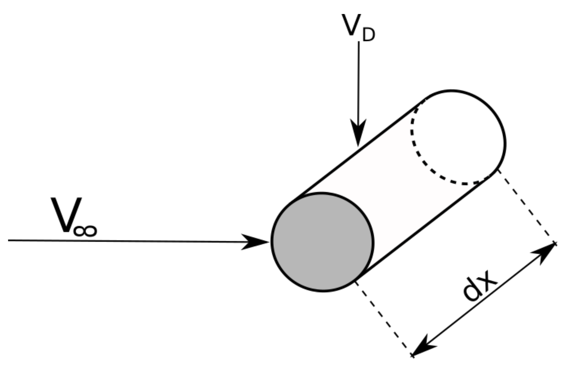
The four central wires have no significant motion during the decaying oscillation, thus their damping contribution can be neglected. The drag force $dF$ exerted on an infinitesimally short wire segment of length $dx$ is:

$$dF=C_{\mathrm{D},\mathrm{cyl}}{D}_{wire}{q}_{\infty }dx,$$

(8)

with the wire diameter $D_{wire}$ and the free-stream dynamic pressure $q_{\infty }$. The only part of $dF$ contributing to $C_{mq}+C_{m\dot{\alpha }}$ is the one acting along the direction of motion of the wire. For small angles this can be approximated by:

$$d{F}_D\left(t\right)\approx dF\frac{v_D}{V_{\infty }},$$

(9)

with

$$v_D=b\frac{x}{L}\dot{\theta }\left(t\right),$$

(10)

being the velocity of the infinitesimal wire element. b is the distance between the wire attachment point on the model and the model’s center of rotation, x is the position of the infinitesimal element along the wire and L the total wire length. The wire element is sketched in Figure 7. Integrating $d{F}_D$ along x gives:

$$F_D={\int }_0^{L}d{F}_D\left(t\right)=\frac{C_{\mathrm{D},\mathrm{cyl}}{D}_{wire}{q}_{\infty }bL\dot{\theta }\left(t\right)}{2V_{\infty }},$$

(11)

with $v_D$ being 0 at the wall attachment point and linearly increasing towards the model, $d{F}_D\left(x\right)$ has a triangular shape. Thus, the load taken on on the model side (as opposed to the wall) is $2/3$ of the total load. With the four wires in the horizontal plane all equally contributing, the wire damping moment is:

$$M_D=4\frac{2}{3}b{F}_D.$$

(12)

Using the expression:

$$M_D=q_{\infty }AD{\left(C_{mq}+C_{m\dot{\alpha }}\right)}_{wire}\frac{\dot{\theta }\left(t\right)D}{2V_{\infty }},$$

(13)

the wire contribution to the stability derivative is calculated as:

$${\left(C_{mq}+C_{m\dot{\alpha }}\right)}_{wire}=\frac{8C_{\mathrm{D},\mathrm{cyl}}{D}_{wire}L{b}^2}{3A{D}^2}.$$

(14)

This part is subtracted from the result determined by Equation (4) with the data for $C_{D,cyl}$ taken from [21].

5. Numerical Investigation

As a reference in addition to the data found in the literature, a numerical study is conducted to determine values for $C_{mq}+C_{m\dot{\alpha }}$ for the two models investigated. The transient planar pitching method described in [14] is used to determine the coefficient sum. Additional calculations are done using a modification of the Lunar Coning method introduced in [24] which uses a combined coning and spinning motion to eliminate the contribution of the Magnus moment. As this method is limited to axisymmetric models, it is applied solely to the ANSR model.

All CFD calculations are performed with the commercial Ansys^® Fluent software [25].

5.1. Transient Planar Pitching Method

In this approach a constant small-amplitude oscillation defined by the equation:

$$\alpha \left(t\right)={\alpha }_0+\mathsf{\Theta }sin\left(\omega t\right),$$

(15)

with the constant amplitude $\mathsf{\Theta }$ and the oscillation frequency $\omega$ is imposed on the model. In an unsteady RANS simulation, the pressure- and shear forces on the model surface are recorded over several periods to determine the pitching moment coefficient $C_m\left(t\right)$ at every time step. In a properly converged calculation $C_m$ follows the equation:

$$C_m\left(t\right)=C_{m\alpha }\alpha \left(t\right)+\left(C_{mq}+C_{m\dot{\alpha }}\right)\frac{qD}{2V_{\infty }}$$

(16)

with the pitching angle $\alpha$ and the pitch rate $q=\dot{\alpha }$. As only low-amplitude oscillations ($\mathsf{\Theta }<1^{\circ }$) are considered, the coefficients $C_{m\alpha }$ and $C_{mq}+C_{m\dot{\alpha }}$ are regarded as constant. When plotted over the pitching angle $\alpha \left(t\right)$, Equation (16) describes an elliptic shape, as shown in Figure 8.

By evaluating the values $C_{m+}$ and $C_{m-}$ at the points where the sine term in Equation (15) equals 0, the pitch damping moment coefficient sum can be calculated using the relation:

$$C_{mq}+C_{m\dot{\alpha }}=\frac{C_{m+}-C_{m-}}{2k\mathsf{\Theta }},$$

(17)

with the non-dimensional frequency $k=\frac{\omega D}{2V_{\infty }}$. This method is implemented in Fluent by defining a User-defined Function (UDF) that moves the reference frame according to Equation (15), thus changing the angle of attack over time.

5.2. Combined Coning and Spinning Method

The Lunar Coning motion [26] is characterized by a rotation of the model at incidence greater zero around an axis defined by the vector of the incoming flow and the model moment reference point. Thus, the same side of the model is facing the rotation axis at all times, hence the description ’lunar’. Although a combination of transient roll, pitch and yaw motions, it results in a steady flow field in the body-fixed reference frame. This fact makes this method well suited for numerical investigations. The non-dimensional coning rate $\mathsf{\Omega }$ is defined as:

$$\mathsf{\Omega }=\frac{\omega D}{2V_{\infty }}.$$

(18)

The expression for the yaw moment coefficient for this flow state ($\alpha \ne 0,\beta =0$) is

$$C_n=\alpha C_{n\alpha }+\alpha p{C}_{np\alpha }+r\left(C_{nr}+C_{n\dot{\beta }}\right).$$

(19)

For symmetrical configurations like the ones investigated in this study this can be simplified with $C_{n\alpha }=0$ and $C_{nr}+C_{n\dot{\beta }}=C_{mq}+C_{m\dot{\alpha }}$. The rates p and r can be calculated from the coning rate $\Omega$:

$$\begin{array}{cc}\hfill p=& \mathsf{\Omega }sin\alpha ,\hfill \\ \hfill r=& \mathsf{\Omega }cos\alpha .\hfill \end{array}$$

(20)

Substituting (20) in (19) then leads to an expression for the desired coefficient sum:

$$C_{mq}+C_{m\dot{\alpha }}=\frac{C_n}{\mathsf{\Omega }sin\alpha }-C_{np\alpha }cos\alpha ,$$

(21)

with the Magnus moment coefficient $C_{np\alpha }$, which has to be determined in a separate calculation. As it is small compared to the other terms, it can also be neglected in a first approximation.

A modification [24] allows the direct determination of $C_{mq}+C_{m\dot{\alpha }}$. For this the Magnus moment caused by the rotation $\mathsf{\Omega }$ needs to be neutralized by a counter-rotation ${\mathsf{\Omega }}^{\prime }$ around the model axis with ${\mathsf{\Omega }}^{\prime }=-\mathsf{\Omega }cos\alpha$. However, this modification can only be applied to axisymmetric bodies as otherwise a transient simulation would be necessary, negating the advantage of the Lunar Coning method. For this reason, these simulations are limited to the ANSR model in the present study. The method can be used in Fluent by modifying the no-slip wall boundary condition such that the fluid velocity at the wall equals the local rotational velocity. The main coning motion is implemented by defining a rotating reference frame.

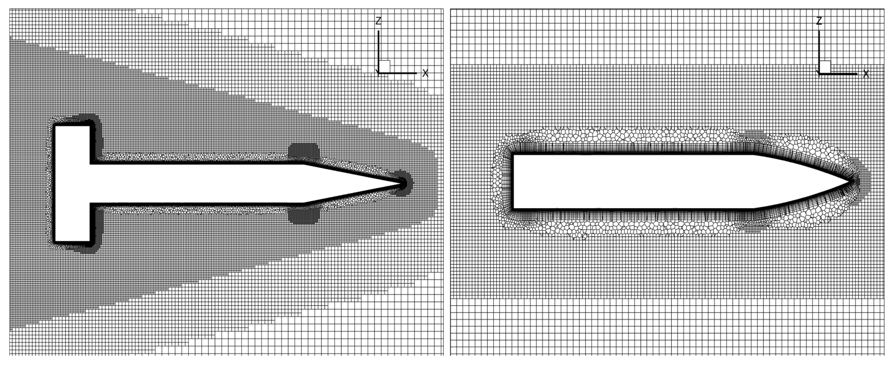
5.3. Numerical Setup

Meshes for both models were created with the Fluent meshing tool. For both models, cylindrical computational domains were used, which extended 250 model diameters downstream of the model. The cylinder radius and the upstream extension were set to 150D. The ANSR mesh consists of $9.3\times {10}^6$ cells, the Basic Finner requires some additional refinement due to the fins, its mesh consists of $16.7\times {10}^6$ cells. Cut plane sections showing the model outlines for both meshes are shown in Figure 9.

A mesh independence study was performed for both models at a Mach number of 0.8 using the transient planar pitching method. The resulting value for $C_{mq}+C_{m\dot{\alpha }}$ obtained on a coarser (ANSR: $2.57\times {10}^6$, Basic Finner: $9.48\times {10}^6$) and a finer (ANSR: $11.46\times {10}^6$, Basic Finner: $19.32\times {10}^6$) mesh were compared to the one obtained on the calculation mesh. The deviations were below 3% on the coarser meshes and below 1% for the finer meshes.

The flow equations are discretized using second-order upwind schemes and are solved with Fluent’s pressure-based solver. The k-$\omega$-SST turbulence model is used. The farfield conditions are chosen based on the flow conditions in the ISL wind tunnel.

For the transient planar pitching method, a non-dimensional oscillation frequency of $k=0.2$ is used, the oscillation amplitude is set to $0.25$ ${}^{\circ }$. The simulation time step is chosen such that there are at least 200 time steps per oscillation period, each time step involving 40 inner iterations. These parameters are chosen based on the parameter study conducted in [14] as well as an own parameter study conducted within the scope of this project.

For the modified Lunar Coning method, the coning rate $\mathsf{\Omega }$ is set to 0.05 and the angle of attack to 3 ${}^{\circ }$. The influence of these parameters was also characterized in a parameter independence study.

6. Results

An extensive test campaign with both models shown in Figure 2 at Mach numbers between 0.6 and 2 has been conducted in the ISL’s trisonic wind tunnel. The extent and the results of the test campaign are summarized below and are discussed in detail.

6.1. Basic Finner

Overall 263 wind-on tests have been conducted with the Basic Finner reference model. The test cases including the relevant test parameters are summarized in

Table 1. Test case conditions for the Basic Finner model.

No.	Wire Attachment	Mach Number	${\mathit{p}}_{\mathbf{tot}}$ [bar]	${\mathit{f}}_0$ [Hz]	Material	Number of Wind-on Tests
1	gripped	0.6	2.0	20.3	steel	15
2	glued	0.6	2.0	21.3	steel	10
3	gripped	0.6	2.0	23.2	steel	15
4	glued	0.6	2.0	24.6	steel	10
5	glued	0.6	2.0	38.2	aluminum	10
6	gripped	0.8	2.0	24.4	steel	15
7	glued	0.8	2.0	25.8	steel	13
8	glued	0.8	1.5	26.1	steel	10
9	glued	0.8	2.0	27.9	steel	12
10	glued	0.8	2.0	44.4	aluminum	10
11	glued	0.9	1.7	25.9	steel	15
12	glued	0.9	1.7	28.2	steel	15
13	glued	0.96	1.7	29.2	steel	12
14	glued	0.99	2.0	30.9	steel	15
15	glued	1.05	2.0	32.0	steel	10
16	glued	1.16	2.3	35.2	steel	15
17	glued	1.16	2.3	57.2	aluminum	7
18	gripped	1.28	2.8	35.4	steel	12
19	glued	1.28	2.8	36.2	steel	15
20	glued	1.28	2.8	60.8	aluminum	6
21	glued	1.46	3.5	37.8	steel	9
22	glued	2.0	2.5	42.7	aluminum	12

. Between test cases 7 and 8, only the wind tunnel total pressure $p_{tot}$ was varied whereas the wire tensioning forces remained unchanged. The higher oscillation frequency $f_0$ is due to the higher additional tension caused by the higher aerodynamic load on the wires.

The results of the present wind tunnel measurements are summarized and compared to the CFD and literature data in Figure 10. The data from references [12,14] are published with a different center of gravity and are thus converted using Equation (5). The coefficients $C_{m\alpha }$, $C_{Z\alpha }$ and $C_{Zq}+C_{Z\dot{\alpha }}$ required for this conversion are taken from [14]. The results agree very well with the CFD results presented in reference [14]. While the free-flight data from reference [12] show a large scatter, particularly in the transonic range, the present wind tunnel measurements are generally within the uncertainty range of these results. The agreement with data from a free-flight test campaign at ISL (partly published in reference [27]) is very good for Mach numbers greater than unity while deviating by approximately 20% at Mach 0.8. The single data point at Mach 2 (test case 20 in Table 1) is slightly lower compared to the wind tunnel tests from reference [11]. In reference [12], the error is given as a percentage of the absolute value for $C_{mq}+C_{m\dot{\alpha }}$ and falls in a range between 10% and 30%. The error bars for the wind tunnel results are calculated using the procedure outlined in Section 4. With a higher number of individual tests, as stated in Table 1, the uncertainties fall in the range of 2% to 8% for most tests. Thus the precision of the experimental measurement is significantly improved.

An excerpt from Figure 10 focusing on the transonic range is shown in Figure 11. The error bars of the free-flight measurements have been removed for clarity and different symbols are used for different model materials and wire attachment methods. In the subsonic range a decrease in $C_{mq}+C_{m\dot{\alpha }}$ can be observed as the Mach number approaches 1, as it is expected based on the literature data. The experimental data indicates a reversal of this trend above Mach 0.9 while the CFD results show the reversal already above Mach 0.8. Using an aluminum model or the gripped wire attachment method does not have a significant impact on $C_{mq}+C_{m\dot{\alpha }}$, although the calculated standard error for the aluminum model is lower compared to the other test cases. Using the CFD data as reference, accuracy in comparison to the free-flight results is improved regardless of the model used.

To better illustrate the influence of the different wire attachment methods and model material, the reference oscillation frequency $f_0$ is plotted over $C_{mq}+C_{m\dot{\alpha }}$ for the test cases at Mach 0.6 in Figure 12 and the test cases at Mach 1.28 in Figure 13. In Figure 12, some tests with the same model configuration but different wire tension forces are shown. For both wire attachment methods, the increase in tension force between the test cases shown is between 60% and 80%. It can be seen that this change only allows for a small modification of the wind-on oscillation frequency. Using the low-inertia aluminum model succeeds in increasing the oscillation frequency significantly. Given the size of the error bars, there is no clear evidence for an influence of the oscillation frequency or the wire attachment method on the stability derivative. The test cases 2 and 4 exhibit a significant difference in measurement error. A similar trend is observed at Mach 0.8 and 0.9. It appears that for this wire attachment method the tensioning force impacts the measurement error, but not the mean value for $C_{mq}+C_{m\dot{\alpha }}$.

The model with the internal gripping mechanism is the only model where the center of rotation is not identical to the center of gravity. Therefore, Equation (5) was used to obtain $C_{mq}+C_{m\dot{\alpha }}$. The necessary values for the coefficients $C_{m\alpha }$ and $C_{Z\alpha }$ are taken from reference [14], the additional uncertainty due to the error propagation is not considered.

6.2. ANSR

Overall, 293 tests were conducted with the Army-Navy Spinner Rocket (ANSR) model. In addition to the configurations with different wire attachment methods, the wire diameter was varied as well. For some test cases at subsonic conditions the four wires at the front and the rear of the model were changed to $0.3$ mm diameter wires or to $0.9$ mm steel cables. The diameter of the four central wires remained fixed at $0.5$ mm. The test cases investigated for the ANSR model are listed in

Table 2. Test case conditions for the ANSR model.

No.	Wire Attachment	Mach Number	${\mathit{p}}_{\mathbf{tot}}$ [bar]	${\mathit{f}}_0$ [Hz]	${\mathit{D}}_{\mathbf{wire}}$ [mm]	Number of Wind-on Tests
1	glued	0.6	2.0	20.6	0.3	8
2	glued	0.6	2.0	21.4	0.5	8
3	gripped	0.6	2.0	22.4	0.5	10
4	glued	0.6	2.0	23.5	0.3	9
5	gripped	0.6	2.0	24.6	0.5	10
6	glued	0.6	2.0	25.1	0.5	10
7	glued	0.6	2.0	27.0	0.9	10
8	glued	0.6	2.0	29.3	0.5	8
9	glued	0.6	2.0	32.0	0.9	10
10	glued	0.8	2.0	19.5	0.3	8
11	glued	0.8	2.0	22.7	0.5	12
12	gripped	0.8	2.0	23.4	0.5	10
13	glued	0.8	2.0	23.8	0.3	8
14	gripped	0.8	2.0	24.4	0.5	10
15	gripped	0.8	1.5	25.2	0.5	8
16	glued	0.8	2.0	25.9	0.5	8
17	glued	0.8	2.0	29.1	0.9	10
18	glued	0.8	2.0	29.7	0.5	8
19	glued	0.8	2.0	32.7	0.9	8
20	glued	0.9	1.7	19.8	0.3	8
21	glued	0.9	1.7	22.8	0.5	8
22	glued	0.9	1.7	23.6	0.3	5
23	gripped	0.9	1.7	24.9	0.5	8
24	glued	0.9	1.7	26.1	0.5	7
25	glued	0.9	1.7	29.7	0.5	8
26	glued	0.9	1.7	29.7	0.9	10
27	glued	0.9	1.7	33.2	0.9	8
28	glued	0.96	1.7	23.9	0.5	10
29	glued	0.99	2.0	24.1	0.5	10
30	glued	1.05	2.0	24.8	0.5	8
31	glued	1.16	2.3	25.0	0.5	8
32	glued	1.28	2.8	24.1	0.5	7
33	gripped	1.28	2.8	24.9	0.5	10
34	gripped	1.37	3.5	25.2	0.5	5

.

The results of the wind tunnel measurements for the ANSR test cases are shown in Figure 14 at different Mach numbers and compared to spark range measurements [13] as well as computational results utilizing both the modified lunar coning method [15,20] and the transient planar pitching method.

The wind tunnel results agree well with the literature and CFD data, especially in the subsonic range. The results show a decrease of $C_{mq}+C_{m\dot{\alpha }}$ with increasing Mach number in the subsonic range, being in good agreement with the results from reference [15]. For supersonic speeds, the absolute value of $C_{mq}+C_{m\dot{\alpha }}$ of the present study increases significantly compared to the subsonic results. Although the literature data also show an increase it is more continuous and less prominent, leading to an underestimation of the stability derivative compared to CFD and spark range results between Mach 1.05 and Mach 1.28. At Mach 1.37 (test case No. 25 in Table 2) the agreement is again within the measurement uncertainties. With the much weaker aerodynamic damping of the ANSR the relative measurement uncertainties are higher than for the Basic Finner, but still within 10% of the absolute value of $C_{mq}+C_{m\dot{\alpha }}$.

Concerning the CFD simulations, a small deviation between the modified lunar coning and the transient planar pitching methods is observed. The transient planar pitching methods results in an approximately 10% lower pitch damping moment coefficient sum compared to the modified lunar coning method, with the exception of the calculations at Mach 0.6, where this trend is reversed. Agreement of the modified lunar coning method with the results published in reference [15] is good. The difference to the data from reference [20] can be explained by the newer, improved turbulence models used in reference [15] and this study.

The magnitude of both the stability derivative itself as well as of the absolute error values is much lower for the ANSR than for the Basic Finner. Thus the correction for the wire damping contribution, as described in Section 4.2, has a much higher impact. This allows an evaluation of the model using the test results obtained with different wire diameters in the subsonic range. Similar to Figure 12, Figure 15 displays the reference frequencies $f_0$ over the stability derivative for the seven different test cases at Mach 0.8 using the glued wire attachment method. For comparison, Figure 16 shows the same results without the wire damping correction. It can be seen that the correction accounts for less than 10% of the total aerodynamic damping if a wire diameter of $0.5$ mm or less is used. Due to the material damping behavior of the steel cables used for the tests at $D_{wire}=$ $0.9$ mm, ${\delta }_{mech}$ is generally higher and not as smooth as the behavior shown in Figure 5. Thus the estimation of the model function ${\tilde{\delta }}_{mech}\left(\mathsf{\Theta }\right)$ is associated with larger uncertainties, leading to the larger error bars in Figure 14 and Figure 15 for these tests. Taking these errors into account, the wire damping model leads to a reasonable correction at Mach 0.6 and Mach 0.8, but not at Mach 0.9. This could be explained by the rougher surface texture of the cables causing the drag coefficient to deviate from the literature values of $C_{D,cyl}$ for smooth cylinders.

Tests at supersonic Mach numbers were not performed with the $0.3$ mm wires as the front wires ruptured during one of the last wind-on tests at Mach 0.9. Since the dynamic pressure was more than double (compared to conditions at Mach 0.9) for all tests at Mach 1.28 and above and no failures occurred with any model equipped with $0.5$ mm wires, this wire diameter is assumed to be a reasonable compromise between mechanical strength and low aerodynamic interference.

The test cases that used the gripped wire attachment mechanism show a decrease in the magnitude of $C_{mq}+C_{m\dot{\alpha }}$ of 15–25%. The measurements with this model were troublesome, particularly the tare measurements showed inconsistencies. A potential reason for these problems and the deviating results is found in the gripping mechanism itself, which, unlike a glued connection, does not enclose the entire circumference of the wire protruding from the model. This is caused by the necessary manufacturing tolerances, which allow the wire some freedom of movement in its notch and cannot be totally eliminated.

6.3. Result Convergence Dependent on the Number of Tests

The statistical approach outlined in Section 4 results in well-converged mean values for $C_{mq}+C_{m\dot{\alpha }}$. To further quantify the influence of the number of wind-on tests, the dependence of the mean and its standard error is analyzed. For selected test cases with N separate wind tunnel test runs, the evaluation is limited to K test runs with $1\le K\le N$. In order to better compare different test cases, the results ${\left(C_{mq}+C_{m\dot{\alpha }}\right)}_K$ as well as the standard error ${\sigma }_{e,K}$ of this partial evaluations are scaled using the results ${\left(C_{mq}+C_{m\dot{\alpha }}\right)}_N$ and ${\sigma }_{e,N}$ of the respective full evaluations:

$$\mathsf{\Xi }=\frac{{\left(C_{mq}+C_{m\dot{\alpha }}\right)}_K-{\left(C_{mq}+C_{m\dot{\alpha }}\right)}_N}{{\sigma }_{e,N}} and\zeta =\frac{{\sigma }_{e,k}}{{\sigma }_{e,N}}.$$

(22)

The number of reference tests to determine the mechanical damping component is unchanged. The scaled pitch damping coefficients $\mathsf{\Xi }$ with the scaled standard errors $\zeta$ for different values of K are shown in Figure 17.

The evaluation procedure was designed for a sufficiently high number of tests, therefore the estimated mean can be outside of the final standard error margin. Nevertheless, already a small number (approx. 3–5) of tests can lead to results close to the converged solution. This is not assured, but through repeat tests and careful observation of the convergence behavior a converged mean value for $C_{mq}+C_{m\dot{\alpha }}$ can be obtained.

6.4. Similarity Considerations

The non-dimensional oscillation frequency $k=\frac{qD}{2V_{\infty }}$ is an important similarity parameter in dynamic tests. Although the stability derivative $C_{mq}+C_{m\dot{\alpha }}$ is assumed to be independent of k in the evaluation process outlined in Section 4, this assumption may not hold for configurations that experience nonlinear effects in flight [10]. Since the experimental approach outlined in this paper provides a mean to vary k to a certain extent, it potentially allows to conduct tests at different values of k if required by designing a model with the correct dimensions and inertia and fine-tuning the oscillation frequency by changing the wire tension forces. It has to be considered that the wire suspension always increases the oscillation frequency that the same model would experience without its influence, e.g., in free flight. Through the correct choice of the model’s material the similarity condition with respect to k can be satisfied.

Through different model materials chosen for the Basic Finner model, the oscillation frequency could be varied by a factor close to 2.

Table 3. Non-dimensional frequency k of the Basic Finner for free-flight and wind-tunnel tests at Mach 0.8.

Free Flight [12]	Free Flight [27]	Wire Suspension (Steel Model)	Wire Suspension (Aluminum Model)
0.0105	0.0053	0.0051 to 0.006	0.0107 to 0.0109

compares k for the Basic Finner wind tunnel tests with the test campaigns from references [12,27] at a Mach number of 0.8. It shows that k is of the same order of magnitude, making the comparison between the different methods valid in terms of the non-dimensional frequency (the wider range of k for the steel model is due to the larger number of tests with different wire tension forces conducted with this model).

7. Conclusions

A wire suspension approach for measuring the pitch damping moment coefficient sum $C_{mq}+C_{m\dot{\alpha }}$ at transonic and low supersonic Mach numbers has been developed. The method minimizes support interference and eliminates the need for expensive measurement equipment integrated into the model. The evaluation process is based on the logarithmic decrement method and accounts for nonlinear terms in the equation of motion. The mechanical damping influence of the wire suspension is determined by the same evaluation process in a tare run without flow. Afterwards, the mechanical damping is used for calculating the aerodynamic damping from the total damping measured at wind-on conditions.

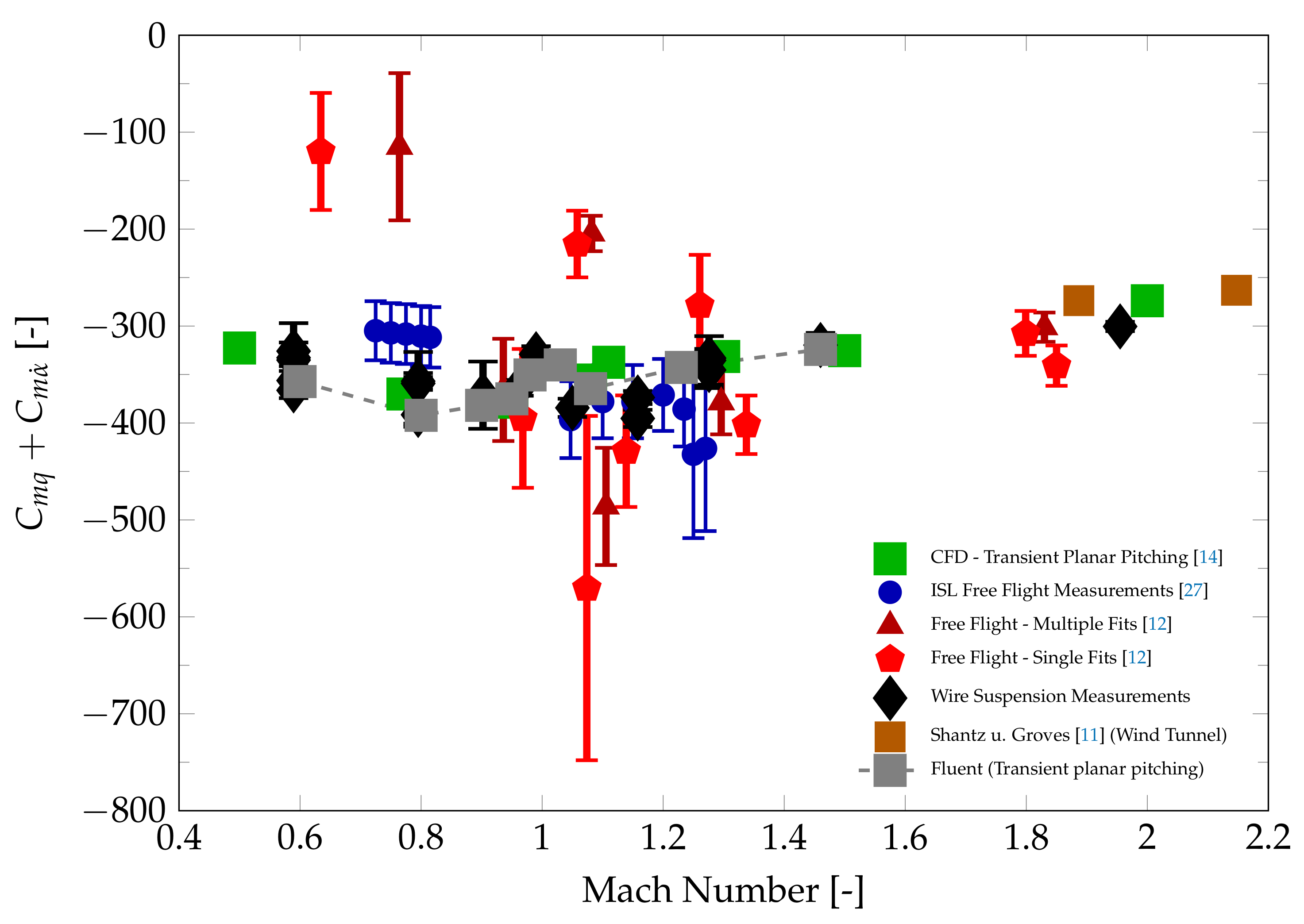
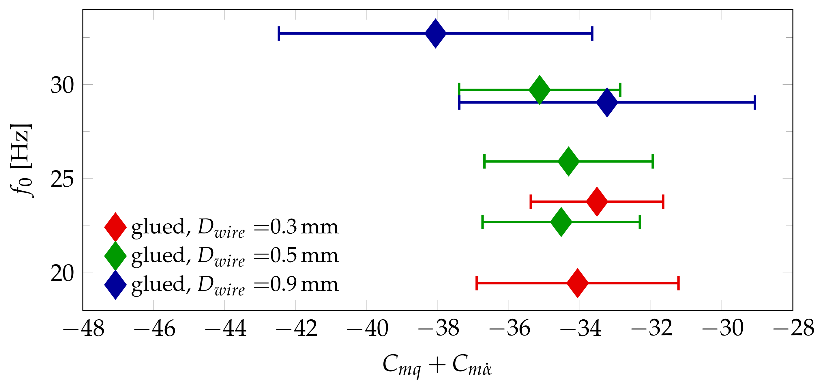
Within an extensive wind tunnel campaign, the presented method has been used to investigate the Basic Finner and ANSR reference models. Their pitch damping coefficients have been measured for Mach numbers ranging from 0.6 to 2. In addition, the influence of oscillation frequency, static pressure, the wire attachment method and the wire thickness has been evaluated.

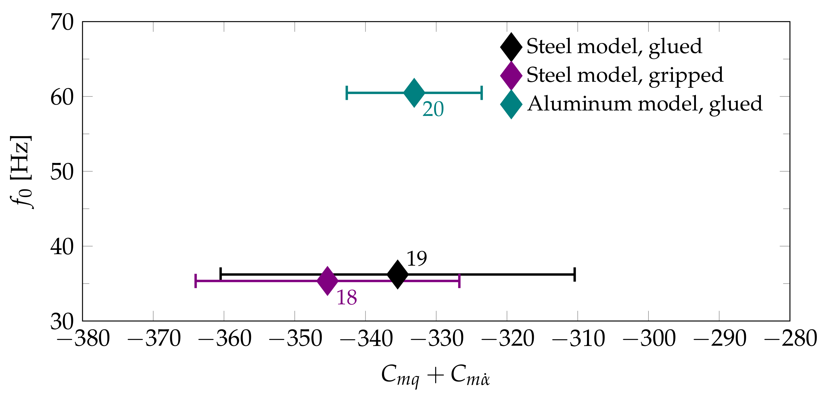
The results show good quantitative agreement for both models with free-flight and CFD data from the literature. In addition, qualitative effects like the increase of $\left|C_{mq}+C_{m\dot{\alpha }}\right|$ with increasing Mach number below Mach 1 as described in the literature are also observable in the present wind tunnel measurements. The wire attachment method and the wire thickness have a small influence, which is nevertheless significant for the ANSR model due to the small magnitude of $C_{mq}+C_{m\dot{\alpha }}$ in that particular case.

Overall, the presented method shows significantly improved accuracy, rendering it a feasible method to determine pitch-damping coefficients in a small-scale supersonic wind tunnel. Therefore, it can help to extend the experimental database for projectile configurations.

References

1. Murphy, C. Free Flight Motion of Symmetric Missiles; Report No. 1216; Ballistic Research Laboratories: Aberdeen Proving Ground, MD, USA, 1963. [Google Scholar]
2. DeSpirito, J.; Silton, S.; Weinacht, P. Navier-Stokes Prediction of Dynamic Stability Derivatives: Evaluation of Steady-State Methods; ARL-TR-4605; Technical Report; U.S. Army Research Laboratory: Aberdeen Proving Ground, MD, USA, 2008. [Google Scholar]
3. McCoy, R.L. The Aerodynamic Characteristics of .50 Ball, M33, API, M8 and APIT M20 Ammunition; Memorandum Report BRL-MR-3810; Ballistic Research Laboratory: Aberdeen Proving Ground, MD, USA, 1990. [Google Scholar]
4. Orlik-Rueckemann, K.J. AGARD Lecture Series 114—Dynamic Stability Parameters; von Kármán Institute for Fluid Dynamics: Rhode-Saint-Génèse, Belgium, 1981. [Google Scholar]
5. Samardzic, M.; Isakovic, J.; Anastasijevic, Z.; Marinkovski, D. Apparatus for Measurement of Pitch and Yaw Damping Derivatives in High Reynolds Number Blowdown Wind Tunnel. Measurement 2013, 46, 2457–2466. [Google Scholar] [CrossRef]
6. Goethert, B.H. Transonic Wind Tunnel Testing; Dover Publications, Inc.: Mineola, NY, USA, 1961. [Google Scholar]
7. Damljanovic, D.; Vukovic, D.; Ocokoljic, G.; Isakovic, J.; Rasuo, B. A Study of Wall Interference Effects in Wind-Tunnel Testing of a Standard Model at Transonic Speeds. In Proceedings of the 30th Congress of the International Council of the Aeronautical Sciences, Daejeon, Korea, 25–30 September 2016. [Google Scholar]
8. Trieu, B.; Tyler, T.; Stewart, B.; Charnock, J.; Fisher, D.; Heim, E.; Brandon, J.; Grafton, S. Development of a Forced Oscillation System for Measuring Dynamic Derivatives of Fluidic Vehicles. In Proceedings of the 38th Aerospace Mechanisms Symposium, Hampton, VA, USA, 17–19 May 2006. [Google Scholar]
9. Franzmann, C.; Leopold, F.; Mundt, C. Experimental Determination of Pitch Damping Coefficients Using a Wire Suspension. In Proceedings of the AIAA SciTech Forum, Virtual Event, 11–15 & 19–21 January 2021. [Google Scholar] [CrossRef]
10. Owens, D.B.; Brandon, J.M.; Croom, M.A.; Frenaux, C.M.; Heim, E.H.; Vicroy, D.D. Overview of Dynamic Test Techniques for Flight Dynamic Research at NASA Langley Research Center. In Proceedings of the 25th AIAA Aerodynamic Measurement Technology and Ground Testing Conference, San Francisco, CA, USA, 5–8 June 2006. [Google Scholar] [CrossRef]
11. Shantz, I.; Groves, R.T. Dynamic and Static Stability Measurements of the Basic Finner at Supersonic Speeds; NAVORD Report 4516; U.S. Naval Ordnance Laboratory: White Oak, MD, USA, 1960. [Google Scholar]
12. Dupuis, A. Aeroballistic Range and Wind Tunnel Test of the Basic Finner Reference Projectile from Subsonic to High Supersonic Velocities; TM 2002-136; Defence R&D Canada: Valcartier, QC, Canada, 2002. [Google Scholar]
13. Schmidt, L.E.; Murphy, C.H. The Aerodynamic Properties of the 7-Caliber Army-Navy Spinner Rocket in Transonic Flight; MR 775; US Army Ballistic Research Laboratories: Aberdeen Proving Ground, MD, USA, 1954. [Google Scholar]
14. Bhagwandin, V.A.; Sahu, J. Numerical Prediction of Pitch Damping Stability Derivatives for Finned Projectiles. J. Spacecr. Rocket. 2014, 51, 1603–1618. [Google Scholar] [CrossRef]
15. DeSpirito, J. CFD Prediction of Magnus Effect in Subsonic to Supersonic Flight; ARL-TR-4929; U.S. Army Research Laboratory: Aberdeen Proving Ground, MD, USA, 2009. [Google Scholar] [CrossRef]
16. Allen, J.; Ghoreyshi, M. Forced Motions Design for Aerodynamic Identification and Modeling of a generic Missile Configuration. Aerosp. Sci. Technol. 2018, 77, 742–754. [Google Scholar] [CrossRef]
17. Libsig, M.; Martinez, B.; Juncker, J.; Bastide, M.; Demeautis, C. Accuracy Enhancement of Wind Tunnel Aerodynamic Coefficients Determination Based on the Coupling of Balance Data and Optical Angle of Attack Measurement. In Proceedings of the 18th International Symposium on Flow Visualization, Zurich, Switzerland, 5 October 2018. [Google Scholar] [CrossRef]
18. Christopher, P.; Brocklehurst, A. A Generalized Form of an Approximate Solution to a Strongly Nonlinear, Second Order Differential Equation. Int. J. Control 1974, 19, 831–839. [Google Scholar] [CrossRef]
19. Greene, W.H. Econometric Analysis, 5th ed.; Pearson-Prentice Hall: Upper Saddle River, NJ, USA, 2002. [Google Scholar]
20. Weinacht, P. Prediction of Pitch-Damping of Projectiles at Low Supersonic and Transonic Velocities. In Proceedings of the 36th AIAA Aerospace Sciences Meeting and Exhibit, Reno, NV, USA, 12–15 January 1998. [Google Scholar]
21. Gowen, F.; Perkins, E. Drag of Circular Cylinders for a wide Range of Reynolds Numbers and Mach Numbers; NACA Technical Note 2960; Ames Aeronautical Laboratory: Moffett Field, CA, USA, 1953. [Google Scholar]
22. Ackerman, J.R.; Gostelow, J.P.; Rona, A.; Carscallen, W.E. Base Pressure Measurements on a Circular Cylinder in Subsonic Cross Flow. In Proceedings of the 38th Fluid Dynamics Conference and Exhibit, Seattle, DC, USA, 23–26 June 2008. [Google Scholar]
23. Shirani, E. Compressible Flow Around a Circular Cylinder. Pak. J. Appl. Sci. 2001, 1, 472–476. [Google Scholar] [CrossRef] [Green Version]
24. Weinacht, P.; Sturek, W.B.; Schiff, L.B. Navier-Stokes Prediction of Pitch Damping for Axisymmetric Projectiles. J. Spacecr. Rocket. 1997, 34, 753–761. [Google Scholar] [CrossRef]
25. ANSYS, I. Ansys® FLUENT, Release 20.0. In FLUENT Theory Guide; ANSYS, Inc.: Canonsburg, PA, USA, 2020. [Google Scholar]
26. Schiff, L.B. Nonlinear Aerodynamics of Bodies in Coning Motion. AIAA J. 1972, 10, 1517–1522. [Google Scholar] [CrossRef]
27. Identification of Aerodynamic Coefficients from Free-Flight Data. Ph.D. Thesis, University of Lorraine, Nancy, France, 2015.
Figure 1. Sketch of the wire suspension geometry.
Aerospace 09 00051 g001
Figure 2. Basic Finner (top) and ANSR (bottom) – all dimensions referenced to calibers.
Aerospace 09 00051 g002
Figure 3. Wire suspension setup in the ISL’s trisonic wind tunnel.
Aerospace 09 00051 g003
Figure 4. Pitch angle over time (left) and δ N measurements over oscillation amplitude Θ (right) for a test with the ANSR model at Mach 0.9.
Aerospace 09 00051 g004
Figure 5. δ m e c h (x) and δ t o t (+) measurements for the ANSR at Mach 0.9.
Aerospace 09 00051 g005
Figure 6. Least-squares fit to data to obtain stiffness coefficients based on Equation (6).
Aerospace 09 00051 g006
Figure 7. Infinitesimal wire element.
Aerospace 09 00051 g007
Figure 8. Typical shape of C m ( t ) over α ( t ) .
Aerospace 09 00051 g008
Figure 9. Mesh refinement around the model for the Basic Finner (left) and the ANSR (right).
Aerospace 09 00051 g009
Figure 10. Wire suspension measurements in comparison with CFD and free-flight data.
Aerospace 09 00051 g010
Figure 11. C m q + C m α ˙ over Mach number for the Basic Finner model – transonic range.
Aerospace 09 00051 g011
Figure 12. Oscillation frequency over C m q + C m α ˙ for the Basic Finner at Mach 0.6 (numbers according to Table 1).
Aerospace 09 00051 g012
Figure 13. Oscillation frequency over C m q + C m α ˙ for the Basic Finner at Mach 1.28 (numbers according to Table 1).
Aerospace 09 00051 g013
Figure 14. C m q + C m α ˙ over Mach number for the ANSR model.
Aerospace 09 00051 g014
Figure 15. Oscillation frequency over C m q + C m α ˙ at Mach 0.8.
Aerospace 09 00051 g015
Figure 16. Oscillation frequency over C m q + C m α ˙ at Mach 0.8 without correction calculated with the wire damping model.
Aerospace 09 00051 g016
Figure 17. Convergence of the scaled pitch damping coefficient sum Ξ over the number of individual wind tunnel tests included in the evaluation for selected test cases.
Aerospace 09 00051 g017