2.2. Attitude Kinematics
Since we deal with an Earth-pointing spacecraft in this work, the focus will be on the kinematics of the spacecraft with respect to the orbital frame. The attitude kinematics equations depend on the representation adopted for the attitude of with respect to .
If the attitude is represented by the following quaternion:
with
, then the attitude kinematics is given by the following (see Section 5.5.3 of [
14]):
where
is the
identity matrix, and the notation
for
represents the skew symmetric matrix:
so that for
, it occurs that
.
On the other hand, if the attitude is represented by rotation matrix
, which transforms vectors of coordinates in
into vectors of coordinates in
, then the the attitude kinematics is given by the following (see ([
15], Section 1.4.1)).
The relation between
q and
is given by the following.
Clearly, the following is obtained.
Moreover, since a circular orbit is considered, then
where
n is the constant orbital rate, and, consequently, the following is obtained.
2.3. Attitude Dynamics and Geomagnetic Field
Attitude dynamics can be expressed in a body frame as follows:
where
is the spacecraft inertia matrix,
,
, and
are the body coordinates of the gravity gradient torque, the control torque induced by magnetic coils, and the disturbance torque, respectively.
The gravity gradient torque in body coordinates is given by the following (see ([
14], Section 6.10)):
where
denotes the unit vector corresponding to the
-axis of
resolved in the body frame, which can be expressed as follows:
where the following is the case.
The spacecraft is equipped with three magnetic coils aligned with the
-axes, which generate the following magnetic control torque:
where
is the vector obtained by stacking the magnetic moments of the three coils, and
is the geomagnetic field at the spacecraft expressed in
. Clearly, the relation between
and
is given by the following.
For what follows, it useful to rewrite Equation (
7) in terms of
instead of
. For that purpose, note that from Equations (
5) and (
6) it follows that
. Thus, since
is constant, the following holds.
By using Equation (
3), we obtain the following.
Thus, from Equations (
7)–(
13), we obtain the following.
Let
be the geomagnetic field at spacecraft expressed in inertial frame
and let
be the rotation matrix that transforms vectors of coordinates in
into vectors of coordinates in
. Note that
and
vary with time at least because of the spacecraft’s motion along the orbit. Then, the following is the case:
which shows explicitly the dependence of
on
t. In order to study Equation (
14), it is important to characterize the time-dependence of
, which corresponds to characterizing the time-dependence of
and
. By adopting the so-called inclined dipole model of the geomagnetic field (see ([
16], Appendix H)) and letting
denote the radius of the circular orbit, we obtain the following.
In Equation (
16),
is the total strength of the inclined dipole,
is the spacecraft position vector resolved in
, and
is the vector of the direction cosines of
. The components of vector
are the direction cosines of the Earth’s magnetic dipole expressed in
, which is set equal to the following:
where
is the coelevation of the inclined dipole,
is the Earth average rotation rate, and
is the right ascension of the dipole at time
.
In order to characterize the time dependence of
in (
16), one needs to determine an expression for
, which is the spacecraft’s position vector resolved in
. Define a coordinate system
,
in the orbital plane, for which its origin is at the center of the Earth and with the
axis coinciding with the line of nodes. Then, the position of satellite centre of mass is given by the following:
where
is the argument of the spacecraft at time
. Let
be the orbit inclination and let
dentote the right ascension of the Ascending Node (RAAN) of the orbit (see ([
13], Section 2.6.2)). Then, the coordinates of the satellite center of mass in the inertial frame can be obtained as follows:
where the following:
is the rotation matrix corresponding to a rotation around the
x-axis of magnitude
and the following:
is the rotation matrix corresponding to a rotation around the
z-axis of magnitude
(see ([
13], Section 2.6.2)).
By combining Equations (
16)–(
21), the expression of
can be easily obtained. Moreover, the following holds.
Thus, by using Equation (
15), an explicit expression for
can be derived. It is easy to see that
can be expressed as a sum of sinusoidal functions of
t having different frequencies since sinusoidal functions having angular frequencies
n and
appear in the previous equations.
A simpler model of the geomagnetic field is the axial dipole model in which the Earth’s magnetic dipole is aligned with the Earth’s rotation axis (see [
17]). Thus, the axial dipole model is obtained by setting
in Equation (
16) and by replacing
with
. Using such a model, the expression of
is simplified as follows.
The latter equation shows that the adoption of a simpler model results in a sinusoidal with period .
The spacecraft and orbit data employed in the following numerical study are obtained from [
12]. The geomagnetic field data are obtained from [
17]. Both data are reported in
Table 2.
2.4. Disturbance Torques
The most significant disturbance torques acting on a spacecraft in low Earth orbit are modeled as follows (see [
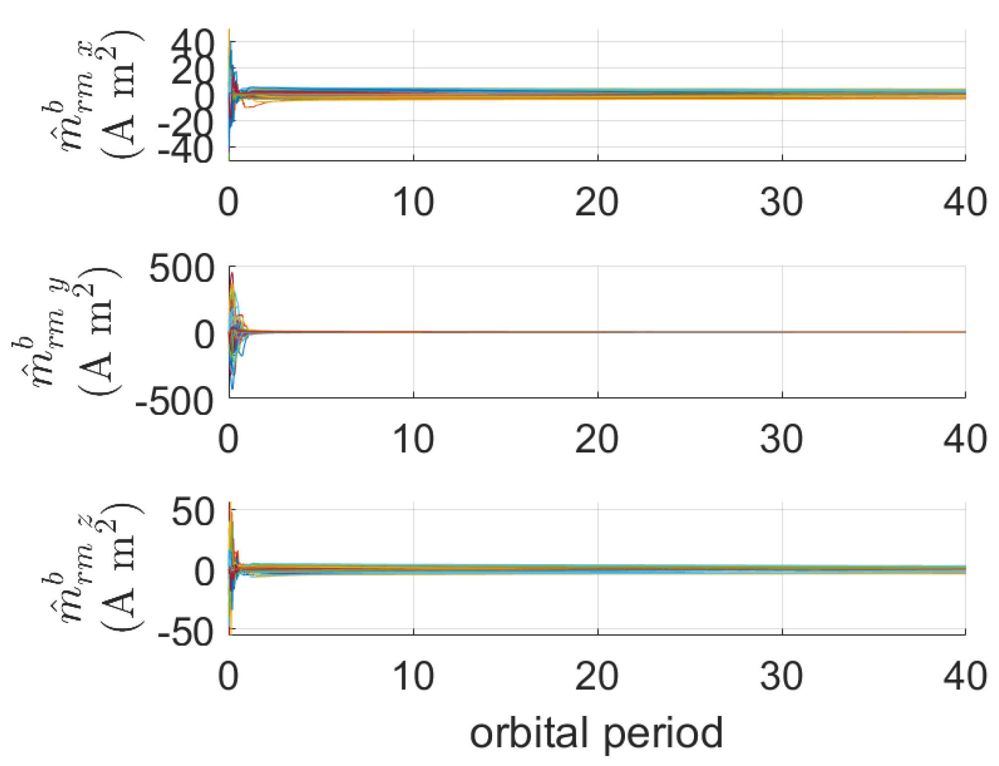
12]). The residual magnetic torque in body coordinates is given by the following:
in which
is the body coordinate of the residual magnetic dipole moment due to onboard electrical components. The aerodynamic torque is modeled as follows:
where
is the body coordinate of the vector from the center of mass to the center of pressure, and
is the body coordinate of the aerodynamic force acting on the spacecraft. A simplified model for
is considered by setting
in which
is the drag coefficient,
is the area of the spacecraft cross section,
is the atmospheric density at orbit altitude, and
is the body coordinate of spacecraft velocity with respect to the air, which is approximated along with spacecraft velocity. The solar radiation pressure torque is modeled as
, where
is the body coordinate of the vector from the center of mass to the center of solar pressure, and
is the body coordinate of the force due to solar radiation pressure, which is modeled as
. In the last equation,
is the solar flux density constant,
c is the speed of light,
is the reflectance factor,
is the area of the sunlit surface, which is assumed constant in the worst case scenario, and
is the body coordinate of the unit vector from the spacecraft to the Sun. Note that
, where
are the coordinates in the inertial frame
of the same unit vector.
The disturbance torques data are obtained from [
12] and reported in
Table 3.


