Article

Performance Enhancement by Wing Sweep for High-Speed Dynamic Soaring

Department of Aerospace and Geodesy, Institute of Flight System Dynamics, Technical University of Munich, Boltzmannstraße 15, 85748 Munich, Germany
*
Author to whom correspondence should be addressed.
Aerospace 2021, 8(8), 229; https://doi.org/10.3390/aerospace8080229
Submission received: 29 June 2021 / Revised: 2 August 2021 / Accepted: 5 August 2021 / Published: 19 August 2021

Abstract

:
Dynamic soaring is a flight mode that uniquely enables high speeds without an engine. This is possible in a horizontal shear wind that comprises a thin layer and a large wind speed. It is shown that the speeds reachable by modern gliders approach the upper subsonic Mach number region where compressibility effects become significant, with the result that the compressibility-related drag rise yields a limitation for the achievable maximum speed. To overcome this limitation, wing sweep is considered an appropriate means. The effect of wing sweep on the relevant aerodynamic characteristics for glider type wings is addressed. A 3-degrees-of-freedom dynamics model and an energy-based model of the vehicle are developed in order to solve the maximum-speed problem with regard to the effect of the compressibility-related drag rise. Analytic solutions are derived so that generally valid results are achieved concerning the effects of wing sweep on the speed performance. Thus, it is shown that the maximum speed achievable with swept wing configurations can be increased. The improvement is small for sweep angles up to around 15 deg and shows a progressive increase thereafter. As a result, wing sweep has potential for enhancing the maximum-speed performance in high-speed dynamic soaring.

1. Introduction

Dynamic soaring is a non-powered flight technique by which the energy required for flying is gained from a horizontal shear wind [1,2]. This type of wind shows changes in the wind speed with the altitude. For sustained dynamic soaring, a minimum in the strength of the wind shear is necessary [3].
There are different modes of dynamic soaring which are associated with features of the shear wind. These features concern the strength of the shear in terms of the magnitude of the wind gradient, the vertical extension of the shear layer or the wind speed level. Shear wind scenarios enabling high-speed dynamic soaring show a thin shear layer and a large difference in the wind speeds above and below the layer. This type of shear wind exists at the leeside of ridges which features a region of large wind speed above the layer and a region of zero or low wind speed below the layer [4].
Theoretical studies and flight experience have shown that it is possible to achieve extremely high speeds with dynamic soaring by exploiting the wind energy relating to the addressed shear layer at ridges [4,5,6,7]. The efficiency of dynamic soaring for transferring wind energy into the kinetic and potential energy of the soaring vehicle manifests in the fact that the speed of the vehicle is many times larger than the wind speed, yielding values of the order of 10 for the ratio of these speeds [8,9].
The high-speed performance enabled by dynamic soaring has stimulated successful speed record efforts over the years to increase continually the maximum-speed level, with the result that the current record is 548 mph (245 m/s) [10]. This highlights the unique capability of dynamic soaring to enable extremely high speeds by a purely engineless flight maneuver.
The experience gained in high-speed dynamic soaring of gliders at ridges is an item of interest for other engineless aerial vehicle types. This can relate to initial testing of dynamic soaring where the strong shear, easy access and relatively obstruction-free environment makes ridge shears attractive. The possibility of gaining energy from the wind so that engineless flight is feasible has stimulated research interest in using the wind as an energy source for technical applications. Evidence for this perspective is found in biologically inspired research and development activities directed at utilizing the dynamic soaring mode of albatrosses for aerial vehicles [11,12,13,14,15,16,17,18].
The aforementioned speed record translates to a Mach number of greater than M a = 0.7 . It can be assumed that this speed is not the top speed as for safety reasons the speed recording is in a section of the dynamic soaring loop after the glider has reached the lowest altitude and is climbing upwind again. Accordingly, the greatest Mach number of the loop may be even higher than that associated with the record speed of 548 mph [9]. Dynamic soaring at such high Mach numbers poses specific problems unique for soaring vehicles because the compressibility effects existing in the Mach number region above M a = 0.7 have an adverse, limiting effect on the achievable maximum-speed performance.
The reason for the addressed limiting effect on the speed performance is due to the drag rise caused by compressibility. The compressibility-related drag rise which is associated with the development of shock waves shows a rapid increase in the drag with the result that the lift-to-drag ratio falls abruptly [19]. The problem concerning the penalty in the speed performance caused by the compressibility-related drag rise is dealt with in [20] and it is shown that it can be so powerful as to yield a limitation in the achievable maximum-speed performance.
The question is whether wing sweep is a solution for the maximum-speed limitation problem. The reason for this consideration is that wing sweep is a means for alleviating compressibility-related drag rise problems in aerospace vehicles by shifting the drag rise to higher Mach numbers.
The purpose of this paper is to deal with increasing the maximum speed enabled by dynamic soaring in the high subsonic Mach number region. To that end, the problems associated with compressibility are addressed and solutions for increasing the maximum speed are derived. Wing sweep is considered as a suitable means to enhance the maximum-speed performance in high-speed dynamic soaring. The focus of this paper is on the development and use of appropriate mathematical models for the flight mechanics of the soaring vehicle at high speeds and the shear wind characteristics, including a suitable optimization method for achieving solutions of the maximum-speed problem. With these developments, analytic solutions are derived, and it is shown that and to what extent the maximum speed can be increased using wing sweep. It is found that the improvement is small for sweep angles up to around 15 deg and shows a progressive increase thereafter.

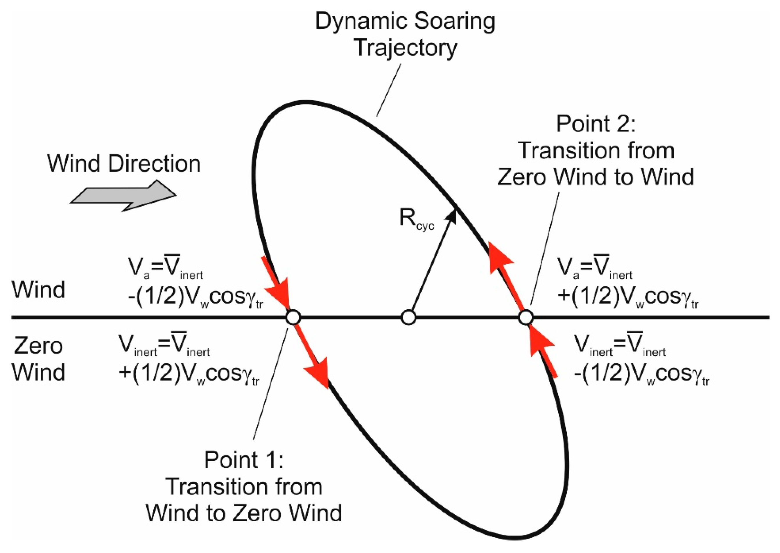
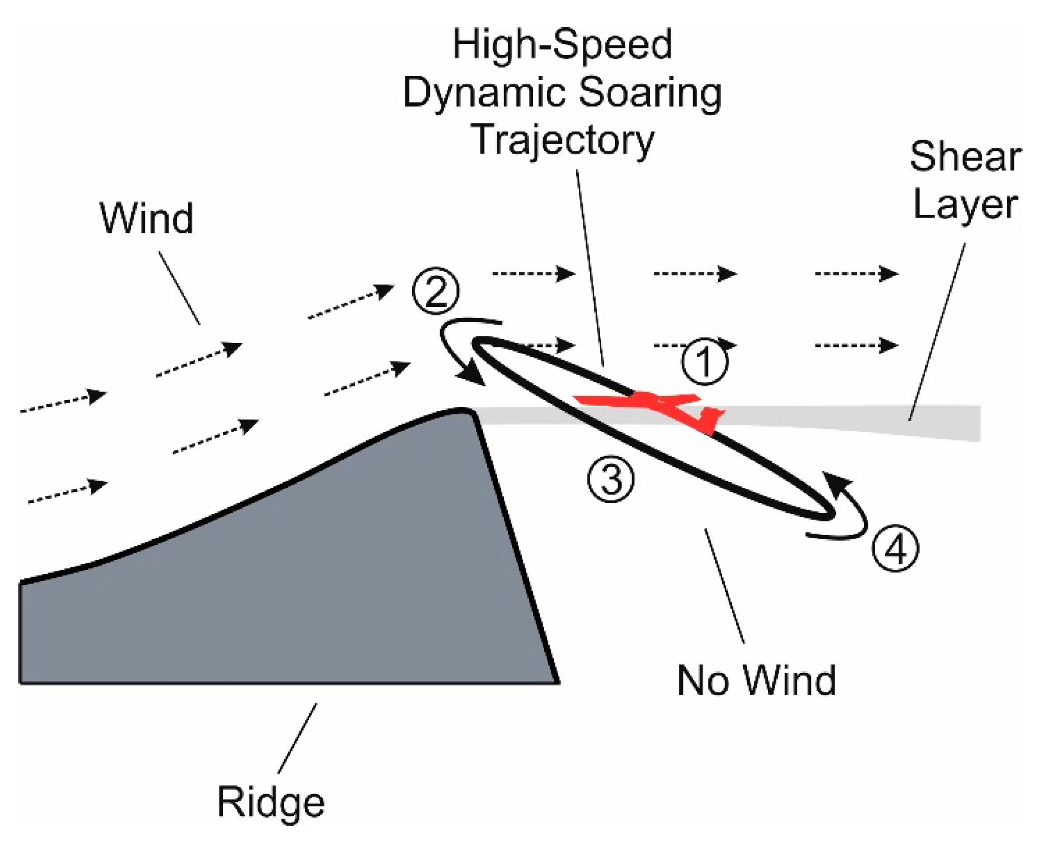
2. Flight Mechanics Modellings of High-Speed Dynamic Soaring

The maximum-speed dynamic soaring problem under consideration is graphically addressed in Figure 1 where a shear wind scenario at a ridge and a dynamic soaring trajectory are shown.
The wind blows at high speed over the ridge, to the effect that there are three regions leeward of the ridge: upper region of high wind speed, thin shear layer showing transition of the wind speed from the region above the layer to the region below the layer and a lower region with no wind or only small wind speeds.
The dynamic soaring trajectory presented in Figure 1 has a shape that enables high speeds by gaining energy from the wind. The trajectory consists of an inclined closed loop showing four flight phases (indicated by nos. 1 to 4), yielding:
(1)
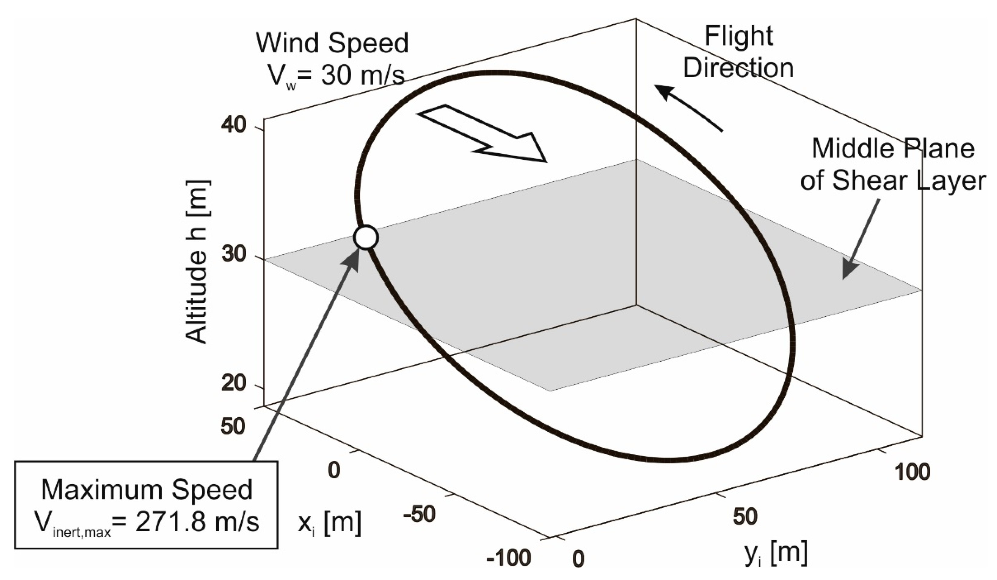
Windward climb where the wind shear layer is traversed upwards.
(2)
Upper curve in the region of high wind speed, with a flight direction change from windward to leeward.
(3)
Leeward descent where the wind shear layer is traversed downwards.
(4)
Lower curve in the no wind region, with a flight direction change from leeward to windward.
The model developed for the shear wind scenario at ridges comprises the described three wind regions. The shear layer involves a rapid increase of the wind speed from zero to the value of the free stream wind speed which is denoted by V w , r e f .
For dealing with the dynamic soaring problem under consideration, two flight mechanics models are developed. One model denoted by “3-DOF dynamics model” is based on point mass dynamics and the other model denoted by “energy model” is based on the energy characteristics determinative in high-speed dynamic soaring. Results applying the 3-DOF dynamics model are used to validate the energy model.

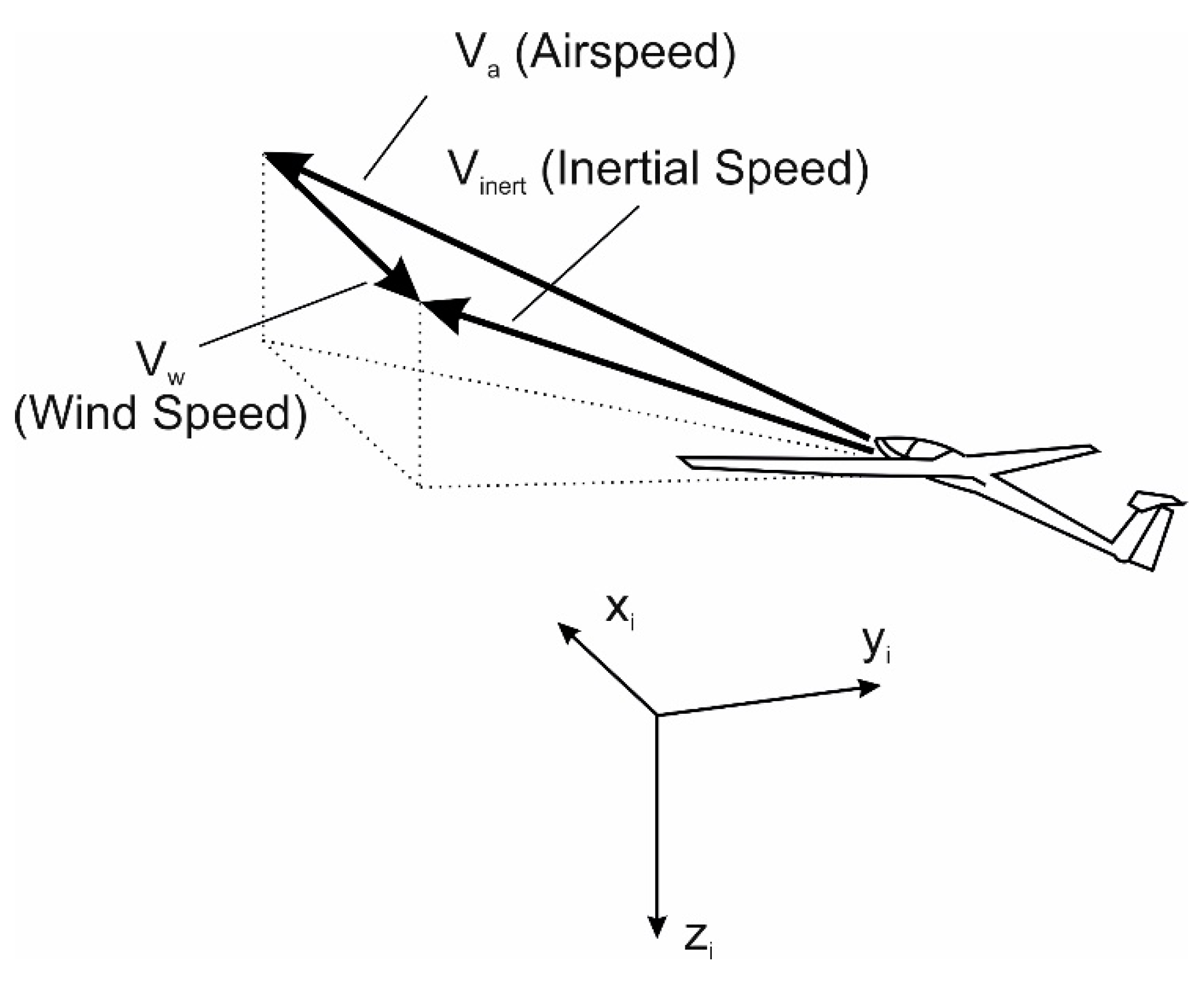
2.1. 3-DOF Dynamics Model

The motion of aerial vehicles in high-speed dynamic soaring can be mathematically described using a point mass dynamics model. An inertial reference system which is presented in Figure 2 is applied where the x i axis is parallel to the wind speed, the y i is horizontal and z i is pointing downward. With regard to this reference system, the equation of motion can be expressed as
d u i / d t = a u 1 D / m a u 2 L / m
d v i / d t = a v 1 D / m a v 2 L / m
d w i / d t = a w 1 D / m a w 2 L / m + g
d x i / d t = u i
d y i / d t = v i
d h / d t = w i
The coefficients a u 1 , 2 , a v 1 , 2 and a w 1 , 2 are abbreviation factors used for describing relationships regarding the angles γ a , μ a and χ a , yielding
a u 1 = cos γ a cos χ a
a u 2 = cos μ a sin γ a cos χ a + sin μ a sin χ a
a v 1 = cos γ a sin χ a
a v 2 = cos μ a sin γ a sin χ a sin μ a cos χ a
a w 1 = sin γ a
a w 2 = cos μ a cos γ a
The angles γ a and χ a are determined by the following relations:
sin γ a = w i / V a
tan χ a = v i / ( u i + V w )
The angle μ a is a control that is determined by the optimality conditions, described by Equation (A2) in the Appendix A.
The aerodynamic forces, L and D , are related to the airspeed vector V a , while the motion of the vehicle is described by the inertial speed vector
V i n e r t = u i , v i , w , T
which is related to the inertial reference system ( x i , y , z i ). The speed vectors V a and V i n e r t are connected by the wind speed vector V w (Figure 2), yielding
V a = V i n e r t V w
The x i axis can be chosen to be in the opposite direction of the wind speed vector V w (Figure 2), with no loss of generality. Thus, the wind speed vector can be written as
V w = V w , 0 , 0 T
With reference to this expression and to Equation (3), the following relations hold true for the airspeed
V a = u i + V w , v i , w , T
and
V a = u i + V w 2 + v i 2 + w i 2

2.2. Energy Model

For developing an energy model valid for the flight mechanics of high-speed dynamic soaring, assumptions on the trajectory and speeds are made. To this aim, reference is made to Figure 3 which provides an oblique view on a dynamic soaring loop. It is assumed that the dynamic soaring loop is circular and the inclination is small. The wind speed is supposed to be smaller than the inertial speed and the airspeed by an order of magnitude, yielding
V w V i n e r t ,   V w V a
Furthermore, the shear layer thickness is assumed to be infinitesimally small.
When traversing the shear layer, there is an approximate speed increase of 1 / 2 V w cos γ t r for the inertial speed in the leeward descent (transition point 1)
V i n e r t = V ¯ i n e r t + 1 2 V w cos γ t r
and for the airspeed in the leeward descent (transition point 2)
V a = V ¯ i n e r t + 1 2 V w cos γ t r
where V ¯ i n e r t is the average inertial speed of the loop and γ t r is the flight path angle at the transition points.
The energy gain from the wind which is necessary for propelling the vehicle is achieved in the upper section of the loop where the wind is blowing. This manifests in an increase of the kinetic energy between the two transition points 1 and 2, yielding
E g = m 2 V ¯ i n e r t + 1 2 V w cos γ t r 2 V ¯ i n e r t 1 2 V w cos γ t r 2 = m V ¯ i n e r t V w cos γ t r
The kinetic energy increase, E g , is equal to the total energy increase since there is no change in the potential energy. This is because the two transition points 1 and 2 are at the same altitude. Furthermore, E g is the net energy increase as the drag work is included in the difference of the total energy between the two transition points in the upper loop section.
The energy gain E g compensates the drag work in the lower loop section. This is the requirement for energy-neutral dynamic soaring.
The drag work in the lower loop section is given by
W D = t 1 t 2 D V i n e r t   d t
where t 1 and t 2 refer to the beginning and end of the lower loop section (associated with the transition points 1 and 2).
The drag work expression can be expanded using the following relation for the drag
D = C D C L L = C D C L n m g
and assuming that the C D / C L ratio and the load factor n are constant. Thus
W D = C D C L n m g s
where
s = π R c y c
is the length of the lower loop section.
The load factor in high-speed dynamic soaring is of the order of n = 100 [5,6,9]. For this n level, the following approximate relation holds true
n = V ¯ i n e r t 2 R c y c g
Thus, the drag work, Equation (14), can be expressed as
W D = π C D C L m V ¯ i n e r t 2
Taking the balance of the drag work and the energy gain into account
E g + W D = 0
and using Equation (11), the average inertial speed of the cycle can be determined to yield
V ¯ i n e r t = 1 π C L C D V w cos γ t r
The speed relationships presented in Figure 3 show that the highest speed in the dynamic soaring cycle is in the leeward descent at the transition point 1, as given by Equation (9). Taking account of this and the fact, that V ¯ i n e r t reaches its greatest value at the maximum lift-to-drag ratio ( C L / C D ) m a x according to Equation (19), the following result on the maximum speed is obtained ( γ t r 1 )
V i n e r t , m a x = 1 2 + 1 π C L C D m a x V w
This is an analytic solution for the maximum speed so that generally valid results concerning the effects of wing sweep can be achieved.
Analyzing the relation Equation (20), the key factors for the maximum speed V i n e r t , m a x can be identified, yielding
(1)
wind speed, V w
(2)
maximum lift-to-drag ratio, ( C L / C D ) m a x
This result shows that there are two key factors. Only one of them is relating to the vehicle. This concerns the aerodynamic characteristics of the vehicle in terms of the maximum lift-to-drag ratio, ( C L / C D ) m a x . It is notable that there is no other vehicle feature (size, mass, etc.) that has an effect on V i n e r t , m a x .
Regarding the wing sweep problem under consideration, the relation Equation (20) shows that ( C L / C D ) m a x is determinative. This means for the aerodynamics influence on the maximum speed that there is only one aerodynamic quantity in terms of ( C L / C D ) m a x that has an effect. As a result, the effect of wing sweep on the speed performance enhancement in high-speed dynamic soaring is determined by the dependence of ( C L / C D ) m a x on wing sweep.

2.3. Straight Wing Reference Configuration (Aerodynamics, Size and Mass Properties)

A straight wing configuration which is representative for modern high-speed gliding vehicles is regarded as a reference and, therefore, will be dealt with first. This is because of two reasons: One reason is to show that there is a limitation of the achievable maximum speed for modern high-speed gliding vehicles which have a straight wing configuration. This limitation is due to compressibility in the high subsonic Mach number region by causing a substantial increase in the drag. The other reason is that the energy model can be validated with results obtained applying the 3-DOF dynamics model. Thus, the energy model can be used to show the performance enhancement achievable with wing sweep for high-speed dynamic soaring.
The aerodynamic forces L and drag D used in the 3-DOF dynamics model and in the energy model can be expressed as
D = C D ρ / 2 V a 2 S
L = C L ρ / 2 V a 2 S
The compressibility-related drag rise in the high subsonic Mach number region manifests in the drag coefficient C D .
Usually, for gliders, the drag coefficient C D shows a dependence only on the lift coefficient C L , but not on the Mach number M a , i.e., C D = C D ( C L ) . This is because the speed of glider type vehicles is comparatively low and associated with the incompressible Mach number region. Concerning high-speed dynamic soaring, however, modern gliding vehicles fly at speeds that can reach the upper subsonic Mach number region. Here, compressibility exerts substantial effects on the aerodynamic characteristics of aerial vehicles, including gliders [9]. An important effect of compressibility in this Mach number region for the performance problem under consideration is a significant rise in the drag. This compressibility-related drag rise manifests in the drag coefficient such that C D shows a dependence on the Mach number M a , in addition to that of the lift coefficient C L , yielding
C D = C D ( C L , M a )
For the high-speed gliding vehicle dealt with in this paper, the drag modelling is graphically addressed in Figure 4. The drag characteristics are shown in terms of drag polars which present the drag coefficient depending on the lift coefficient and the Mach number. This includes the modelling of the induced drag which is based on a quadratic drag-lift relationship, C D = C L 2 / e Λ . The term e is the Oswald efficiency factor for which a value of e = 0.9 is regarded appropriate for the wing under consideration [21]. Furthermore, the contributions of the fuselage and the tail to the drag at zero lift are included in the drag modelling. This contribution amounts to 15 % of the zero-lift drag. Further modelling data concern the wing reference area,   S = 0.51   m 2 , the aspect ratio,   A = 22.5 , and the vehicle mass, m = 8.5   kg . For the described modelling including the drag related compressibility effects, reference is made to existing vehicles and to experience in this field [6,8,22].
The energy model, Equation (20), shows that there is only one aerodynamics quantity that is determinative for the effect of wing sweep on the maximum speed performance. This is the maximum lift-to-drag ratio ( C L / C D ) m a x . Thus, the dependence of ( C L / C D ) m a x on the Mach number M a is determinative for the wing sweep problem under consideration. The dependence of ( C L / C D ) m a x on M a can be determined by an examination of the drag polars depicted in Figure 4.
Results are presented in Figure 5 where ( C L / C D ) m a x dependent on M a is plotted. The ( C L / C D ) m a x curve has a shape that can be subdivided into two parts. In the left curve part, ( C L / C D ) m a x is constant and shows the highest level. Constancy of ( C L / C D ) m a x with regard to M a implies that there is no effect of compressibility. Thus, the left part of the ( C L / C D ) m a x curve can be related to the incompressible M a region. In the right curve part, there is a continual decrease of ( C L / C D ) m a x which rapidly leads to small values. This decrease of ( C L / C D ) m a x is an effect of compressibility, associated with the drag rise described above. Thus, the right part of the ( C L / C D ) m a x curve can be related to the compressible M a region.
The lift coefficient associated with ( C L / C D ) m a x , denoted by C L * , is also presented in Figure 5. The relation between C L * and ( C L / C D ) m a x is given by
C L C D m a x = C L * M a C D C L * M a
The C L * curve has a shape that can also be subdivided into two parts. The left curve part where C L * is constant and highest, can be related to the incompressible M a region. In the right curve part, C L * shows a decrease to approach considerably smaller values which is due to compressibility. Thus, the right curve part can be associated with the compressible M a region.

3. Maximum Speed Achievable with Straight-Wing Configuration

The objective of this Chapter is to validate the energy model developed in the previous Chapter. Thus, the energy model can be used to produce results on the maximum-speed performance.
For validating the energy model, results achieved with the 3-DOF dynamics model are used. These results were produced applying the optimization method described in the Appendix A.

3.1. Maximum-Speed Performance of Straight Wing Reference Configuration

As a reference for the wing sweep problem under consideration, the straight wing configuration described above is dealt with first. An objective is to show characteristic features of the trajectory and relevant motion variables in maximum-speed dynamic soaring. Another objective is to address the effect of compressibility, especially with regard to its limiting influence. For this purpose, a high wind speed scenario showing a wind speed of V w , r e f = 30   m / s is selected, with the result that compressibility is effective throughout the entire dynamic soaring cycle. Furthermore, the treatment of this section is also intended to give an illustrative insight into high-speed dynamic soaring in terms of a highly dynamic flight maneuver.
Results are presented in Figure 6 which provides a perspective view on the optimized closed-loop trajectory. The maximum speed is obtained as V i n e r t , m a x = 271.8   m / s . The picture shows the spatial extension of the trajectory in the longitudinal, lateral and vertical directions and its relation relative to the wind field regarding the wind direction and the shear layer. The trajectory point where V i n e r t , m a x occurs is at about the end of the upper curve. This corresponds with the energy model.
Side and top views of the optimized trajectory are presented in Figure 7. The side view shows that the trajectory projection comprises two lines which are nearly straight and close to each other. This means that the trajectory itself is virtually in a plane. Another feature is that the inclination of the trajectory is small. The top view reveals that the trajectory projection on the x i - y i plane shows a circular-like shape. This feature and the small inclination suggest that the circular characteristic also holds true for the trajectory itself. Furthermore, the side view shows that the extensions of the trajectory above and below the middle plane of the shear layer are practically equal.
The described trajectory characteristics are in accordance with the assumptions made for the trajectory of the energy model, as presented in Figure 3. This accordance contributes to the validation of the energy model.
Compressibility exerts an essential influence on the maximum-speed performance for wind speeds of the current level. An insight on how this influence becomes effective can be gained considering the speed and Mach number characteristics. For this purpose, the inertial speed, V i n e r t and the Mach number, M a , are addressed by presenting their time histories in Figure 8.
The speed curve (the time scale is chosen such that the maximum speed V i n e r t , m a x = 271.8   m / s is at the beginning t = 0 ) shows that V i n e r t features one oscillation the downward part of which is longer than the upward part. The minimum of V i n e r t is at a point of the trajectory where the vehicle has passed the lowest altitude and is climbing upwind again.
The role of compressibility for the problem under consideration becomes evident addressing the Mach number M a reached during the cycle and putting this in relation with the drag polar characteristics of the vehicle. The time history of M a presented in Figure 8 shows that the M a curve comprises two oscillations which are rather similar. Furthermore, the M a level is so high that it relates to the compressible region of the drag coefficient C D throughout the entire cycle. This means with reference to Figure 4 that the drag rise due to compressibility is fully effective. Thus, the maximum-speed performance is negatively influenced at all points of the trajectory.

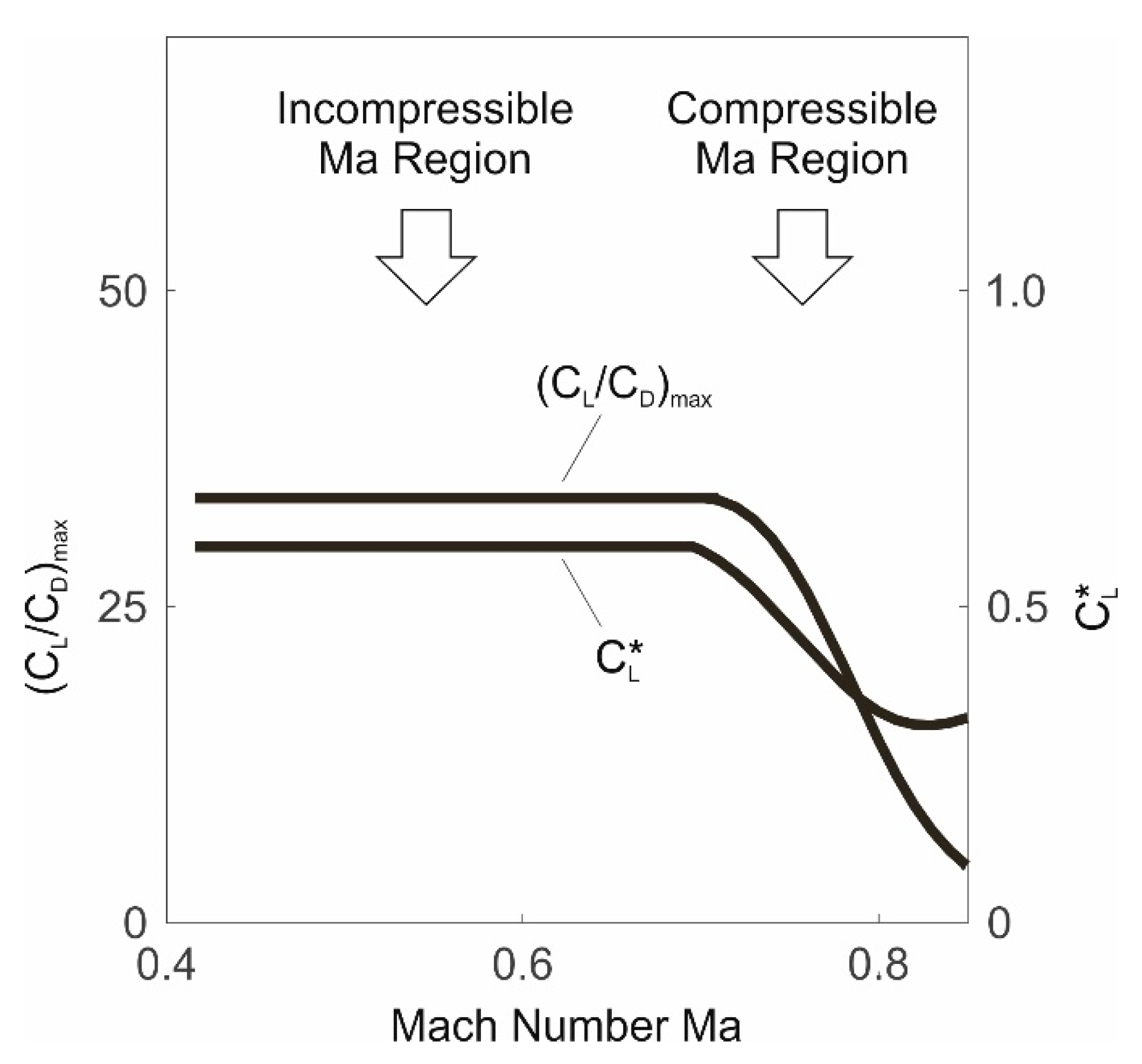
3.2. Maximum-Speed Performance and Related Key Factors

The maximum speed achievable in high-speed dynamic soaring, V i n e r t ,   m a x , is central for the subject under consideration in this paper. There are, according to Equation (20), two key factors for V i n e r t ,   m a x : the wind speed, V w , and the maximum lift-to-drag ratio, ( C L / C D ) m a x . Because of their key factor role, the effects of V w and   ( C L / C D ) m a x on V i n e r t ,   m a x , will be analyzed in detail. Emphasis is put on the role of   ( C L / C D ) m a x as this key factor is determinative for the effect of wing sweep on the maximum speed achievable. This analysis is considered a means for validating the energy model.
Results on the maximum speed are presented in Figure 9 where the dependence of V i n e r t ,   m a x on V w is shown. The range selected for V w is such as to cover a wide spectrum of wind speeds possible at ridges, with the objective to achieve results generally valid for high-speed dynamic soaring.
The dotted line curve shows the results using the 3-DOF dynamics model. Concerning this model, the optimization procedure that is described in the Appendix A was applied to achieve solutions for determining the maximum speed. The solid line curve shows the results using the energy model. Concerning this model, solutions were constructed using Equation (20). Both V i n e r t ,   m a x curves are close to each other and overlap in parts, to the effect that the results of the 3-DOF dynamics model and the energy model approaches virtually agree. This suggests that the energy model Equation (20) is confirmed.
The fact that both model approaches virtually agree manifests in more aspects. This will be shown in the following sections where a detailed treatment on these aspects is presented.
Examining the V i n e r t ,   m a x curve characteristics in Figure 9, the left part of the curve shows a comparatively large and constant gradient, whereas the gradient in the right part is substantially reduced. Relating this property of the V i n e r t , m a x gradient to the Mach number M a indicated on the ordinate shows that the change in the gradient starts in a zone where compressibility begins to become effective for the aerodynamic characteristics of the vehicle. Thus, the left part of the V i n e r t , m a x curves can be related to the incompressible M a region, whereas the right part can be related to the compressible one.
The reason for the fact that there are two different parts in the V i n e r t ,   m a x curve is due to ( C L / C D ) m a x . In the left part of the V i n e r t ,   m a x curve, ( C L / C D ) m a x is constant so that, according to Equation (20), the V i n e r t ,   m a x gradient is also constant, whereas the V i n e r t ,   m a x gradient in the right curve part is substantially reduced. The cause for the reduction of the V i n e r t ,   m a x gradient is due to   ( C L / C D ) m a x . This is because   ( C L / C D ) m a x shows a decrease in the compressible Mach number region. According to Equation (20), a reduction in ( C L / C D ) m a x   leads to a corresponding reduction in V i n e r t , m a x . This means that ( C L / C D ) m a x is the cause for the limitation in the achievable V i n e r t , m a x values.
Further evidence and understanding of the effect of   ( C L / C D ) m a x on V i n e r t , m a x can be provided when analyzing the actual lift-to-drag ratio, C L / C D , during the dynamic soaring cycle and comparing this with the maximum lift-to-drag ratio, ( C L / C D ) m a x , of the same cycle. Results on that issue are plotted in Figure 10.
As each of C L / C D and ( C L / C D ) m a x varies during the cycle, the average values of these quantities are considered as representative. They are given by
C L C D a v = 1 t c y c 0 t c y c C L C D   d t
and
C L C D m a x , a v = 1 t c y c 0 t c y c C L C D m a x   d t
Both quantities have been determined using the 3-DOF dynamics model and the optimization method describes in the Appendix A.
The results presented in Figure 10 address the relationships between the lift-to-drag ratios, ( C L / C D ) m a x , a v and ( C L / C D ) a v and the wind speed, V w . Basically, each of the ( C L / C D ) m a x , a v and ( C L / C D ) a v curves shows two parts. The left parts featuring a constant level are associated with the incompressible Mach number region, whereas the right parts involving a continual decrease are associated with the compressible region.
A main result is that the ( C L / C D ) m a x , a v and ( C L / C D ) a v curves are close to each other and overlap in parts. This means that the actual ( C L / C D ) a v values virtually agree with the maximum lift-to-drag ratio, ( C L / C D ) m a x , a v .
These characteristics of the lift-to-drag ratios ( C L / C D ) a v and ( C L / C D ) m a x , a v are of importance for the energy model. This is because the fact that ( C L / C D ) a v virtually agrees with ( C L / C D ) m a x , a v supports the assumption made for the energy model. Accordingly, it is assumed for the energy model that the maximum lift-to-drag ratio ( C L / C D ) m a x holds true for the maximum speed V i n e r t , m a x , Equation (20).
The main role that ( C L / C D ) m a x plays as the determinative aerodynamics quantity for the maximum speed is further substantiated and confirmed by the broader treatment presented in the following. For this purpose, three different ( C L / C D ) m a x configurations are dealt with and their effects on V i n e r t , m a x are analyzed and compared. The range selected for ( C L / C D ) m a x is larger than the ( C L / C D ) m a x range characteristic for high-speed gliding vehicles.
Results are presented in Figure 11 which shows the relationship between V i n e r t ,   m a x , V w and ( C L / C D ) m a x where the notation ( C L / C D ) m a x , r e f refers to the maximum lift-to-drag ratio configuration applied so far and used as reference. The results show that it can again be distinguished between the left and right parts of each V i n e r t , m a x curve which are related to the incompressible and compressible Mach number regions, respectively. In the left curve parts, there are large differences between the three V i n e r t , m a x curves (for each of the solid and dotted lines) that are due to the effect of   ( C L / C D ) m a x . These differences reflect the strong influence of ( C L / C D ) m a x on V i n e r t ,   m a x , according to the energy model Equation (20). This manifests in a particular manner for the case of the 50% decrease in ( C L / C D ) m a x as the related V i n e r t , m a x curve practically does not reach the Mach number region where compressibility is effective. Further to the left curve parts, comparing the solid lines holding true for the energy model and the dotted lines holding true for the 3-DOF dynamics model shows that they virtually agree.
Concerning the right curve parts, there are two effects valid for the V i n e r t , m a x curves of both ( C L / C D ) m a x cases reaching the compressible Mach number region. Firstly, the V i n e r t , m a x curves (for each pair of solid and dotted lines) show no longer a large difference but are close to each other. Secondly, the increase of V i n e r t , m a x of both ( C L / C D ) m a x cases is substantially reduced and there is practically a limitation of the achievable V i n e r t , m a x values. These two effects are the result of the decrease of ( C L / C D ) m a x due to compressibility (Figure 5). This means that ( C L / C D ) m a x plays the primary role in limiting the achievable V i n e r t , m a x values.
Here, again, the findings of the energy model agree with those of the 3-DOF dynamics model. This is particular important for the compressible Mach number region because the limitation in V i n e r t , m a x is related to that Mach number region.
In summary, the analysis in this Chapter shows that the results of the energy model virtually agree with the results of the 3-DOF dynamics model. The results on the maximum speed and related quantities are close to each other and overlap in parts. This suggests that the energy model is validated so that it can be used in lieu of the 3-DOF dynamics model.

4. Increase of Maximum-Speed Performance by Wing Sweep

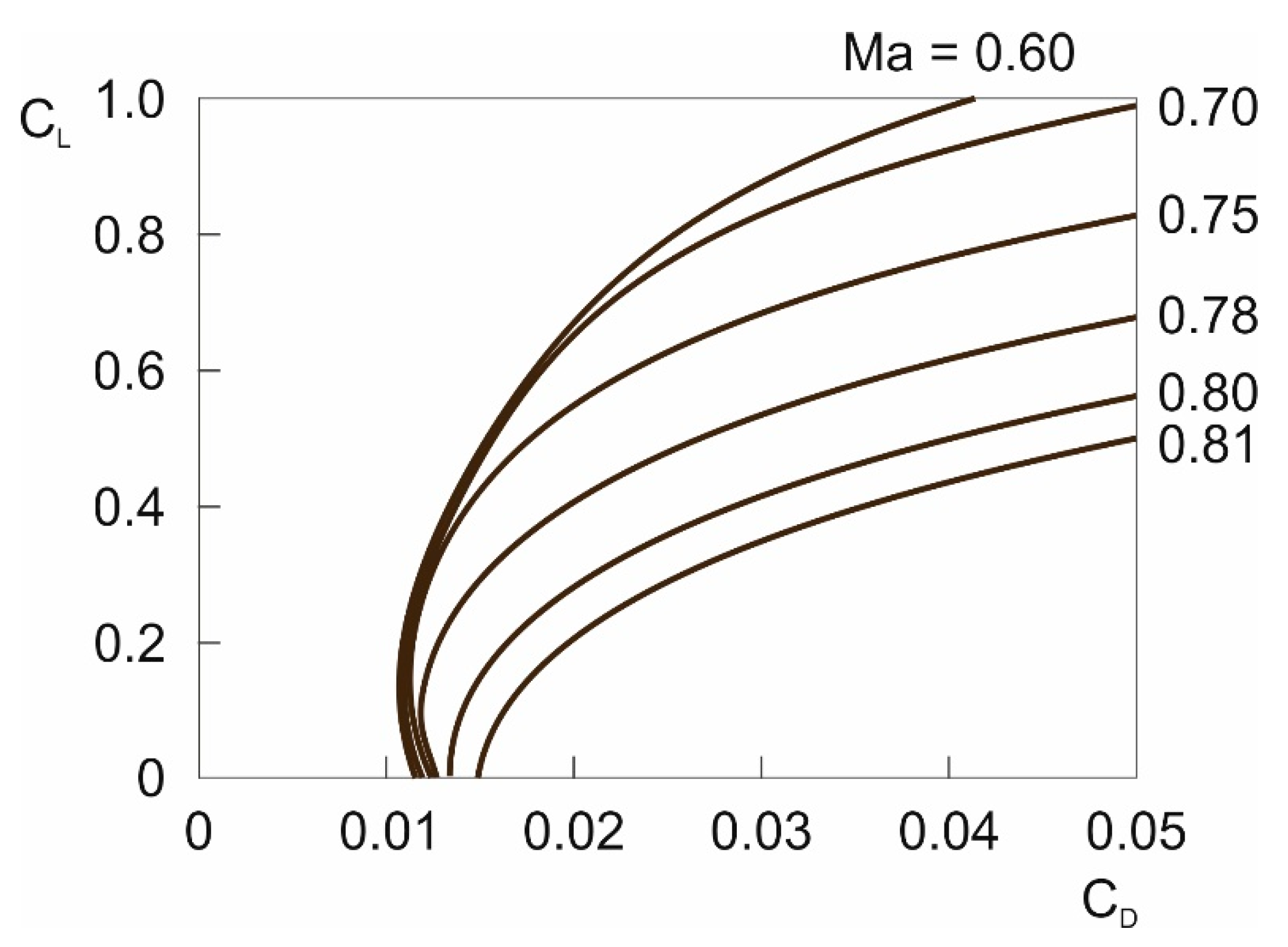
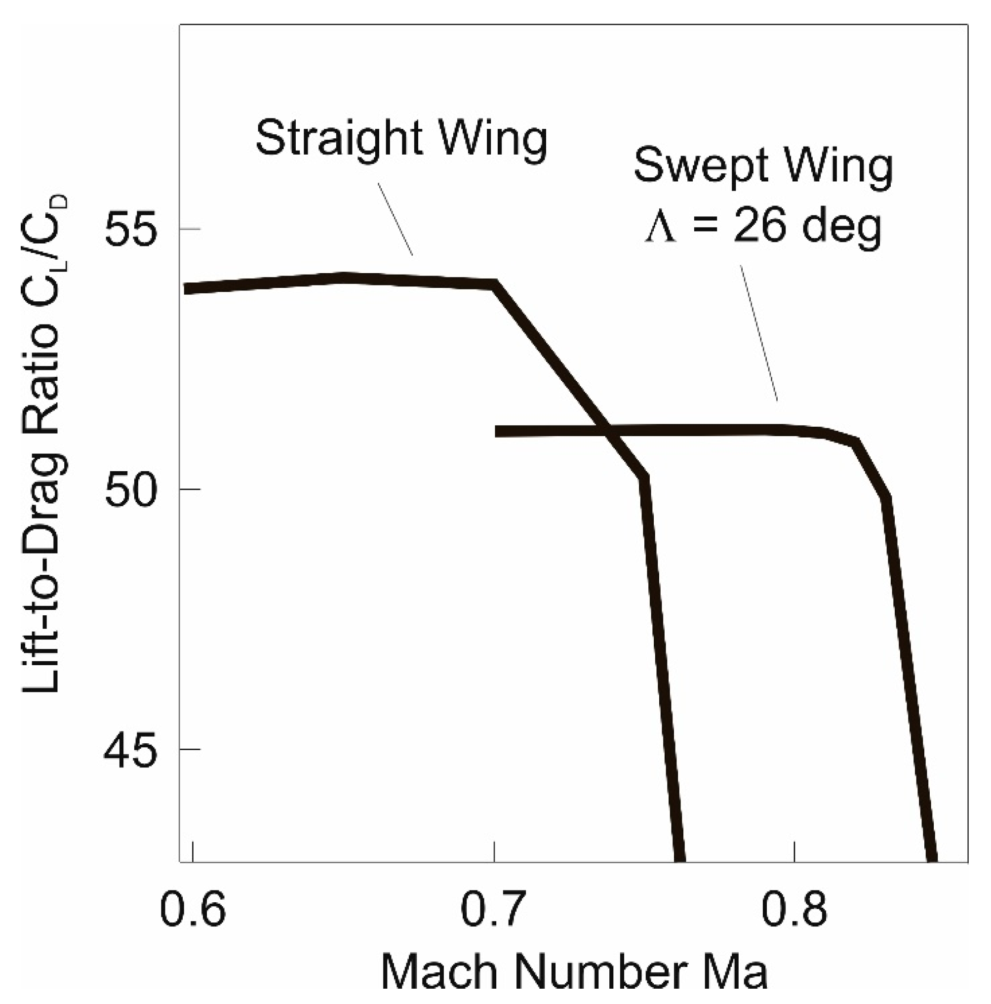
4.1. Aerodynamic Characteristics of Swept Wing Glider Configurations

The results of the previous treatment on the limitation of V i n e r t , m a x for straight wing configurations show that the decrease of ( C L / C D ) m a x caused by compressibility is the reason for this limitation. The limitation begins to become effective at the Mach number at which the compressibility-related drag rise begins. That drag rise is associated with two Mach numbers [21]. One is the critical Mach number, M a c r , which is the Mach number at which the speed of sound is reached at some point of the vehicle. The other one is the drag divergence Mach number, M a d d , which is the Mach number at which the drag coefficient starts to rise rapidly. M a d d is slightly greater than M a c r .
A possible solution of the drag rise problem is wing sweep. This is illustrated in Figure 12 where the lift-to-drag ratio, C L / C D , of a swept wing configuration and of a corresponding straight wing configuration representative for glider type vehicles are shown. The planform of the swept wing configuration is presented in Figure 13.
Figure 12 shows the Mach number region where compressibility causes the C L / C D decrease of the two wing configurations. Concerning the straight wing configuration, the C L / C D decrease begins at about M a 0.7 ÷ 0.75 and the C L / C D ratio shows thereafter a steep gradient to reach rapidly smaller values. Concerning the swept wing configuration, the C L / C D decrease begins at about M a 0.81 ÷ 0.83 . Thereafter, the drag decrease shows a behavior corresponding with that of the straight wing configuration in terms of a similarly steep gradient. Comparing the two cases provides an indication of the possible shift in the drag rise to higher Mach numbers for wings of glider type vehicles.
The following assumptions are made for determining the effects of wing sweep on the maximum-speed performance of high-speed dynamic soaring:
(1)
Energy based model
It is assumed that energy model for high-speed dynamic soaring, Equation (20), can be used for determining the effects of wing sweep on the maximum speed, V i n e r t , m a x . This is based on the results concerning the validation of the energy model.
The energy model Equation (20) shows that the ( C L / C D ) m a x is the only aerodynamic quantity that has an effect on V i n e r t , m a x . Thus, the effect of wing sweep on the speed performance enhancement in high-speed dynamic soaring can be determined by taking the dependence of ( C L / C D ) m a x on wing sweep into account and by incorporating this dependence in Equation (20). For that purpose, the critical Mach number and its relationship with the wing sweep is used to address the dependence of ( C L / C D ) m a x on wing sweep.
(2)
Critical Mach number, M a c r
For the critical Mach number, the following relation is used [19,24,25]
M a c r , Λ = M a c r , 0 cos Λ
where M a c r , Λ refers to the swept wing featuring a sweep angle of Λ and M a c r , 0 refers to the straight wing.
The relation described by Equation (26) is considered as suitable for wings of a large aspect ratio. This is because wings of a large aspect ratio show a characteristic similar to airfoils the characteristic of which is determined by 2-D effects. Accordingly, the 3-D effects near the tip and the root of large aspect ratio wings tend to be small when compared with low aspect ratio wings.
Large aspect ratios are generally used in aerodynamically efficient gliders [26]. This holds true also for gliders in high-speed dynamic soaring [10]. For the type of wings under consideration, the swept wing configuration shown in Figure 13 can be seen as representative and the swept wing configuration 1 (described below), shows an aspect ratio of Λ = 22.5 .
(3)
Maximum lift-to-drag ratio, ( C L / C D ) m a x
The relationship between ( C L / C D ) m a x and M a shown in Figure 5 holds true for the straight wing configuration. The shape of this curve is also used for the swept wing configuration 1 (Figure 14). For that purpose, it is assumed that the ( C L / C D ) m a x curve is horizontally shifted to higher Mach numbers according to the increase of M a c r , Λ compared to M a c r , 0 , using the relationship of Equation (26).
This procedure is based on the following considerations: It is assumed that the swept wing configuration shows the same ( C L / C D ) m a x value as the straight wing configuration in the incompressible Mach number region. This assumption implies that the zero-lift drag coefficients of both wing configurations agree and that an analogue relationship between the lift-dependent drag coefficients holds true. For the equality of the lift-dependent drag coefficients, it is assumed that the spanwise lift distributions of the two wing configurations agree. This is considered to be achievable by an appropriate twist of the wing.
A further aspect for the described procedure is that a main effect of wing sweep on V i n e r t , m a x concerns the beginning of the ( C L / C D ) m a x decrease where the compressibility-related drag rise starts to grow rapidly. This corresponds with the V i n e r t , m a x behavior at the transition of the left and right curve parts in the V i n e r t , m a x diagrams presented in Chapter 3. Here, the increase of V i n e r t , m a x comes nearly to a stop and there is a limitation for the achievable maximum speed.

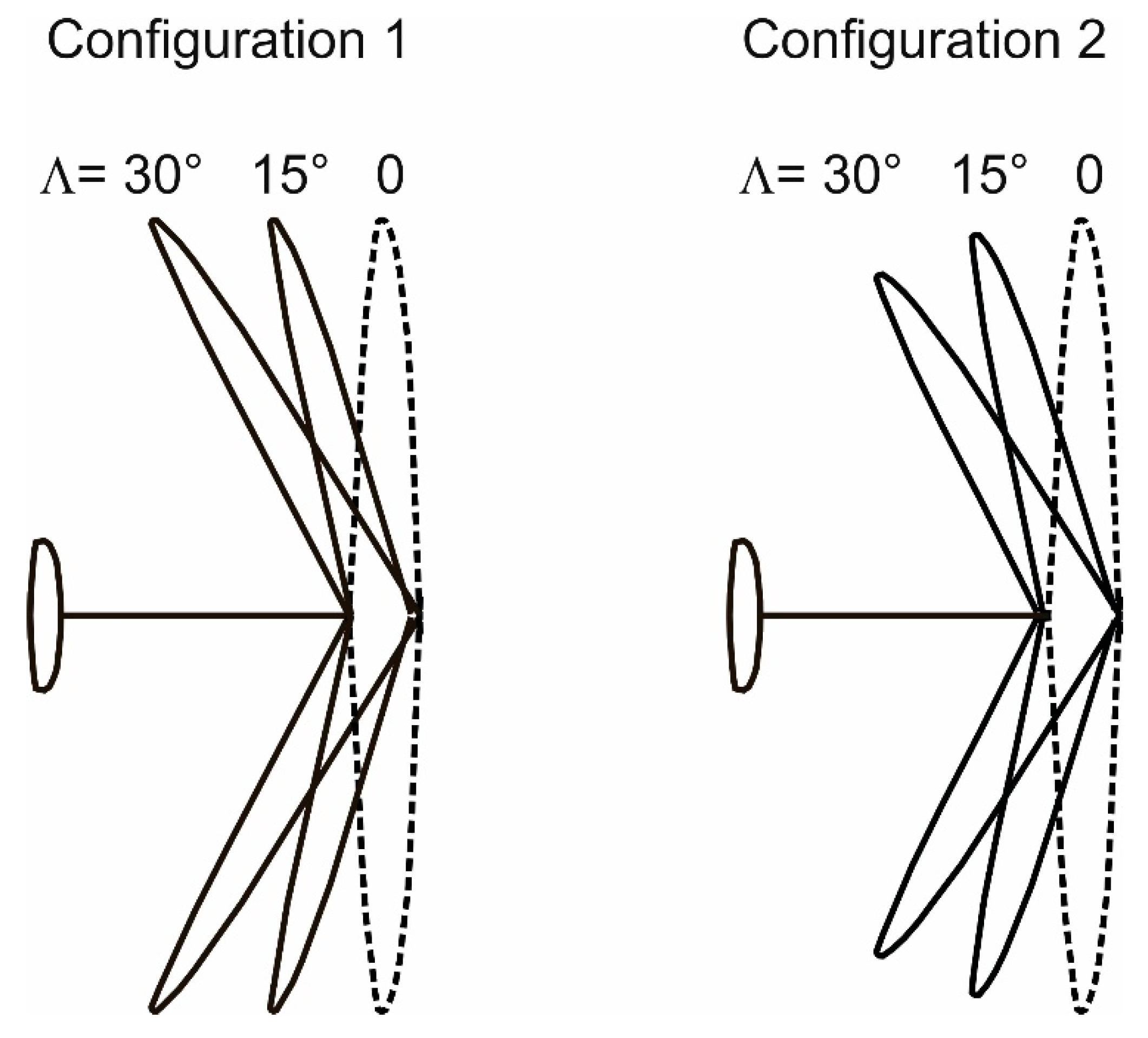
4.2. Swept Wing Configurations

For showing that and how with wing sweep can enhance the speed performance in high-speed dynamic soaring, two swept wing configurations 1 and 2 schematically presented in Figure 14 are dealt with. Each of the two configurations features the same sweep angles in terms of Λ = 15 ° and Λ = 30 ° . A 40 ° sweep angle configuration is additionally addressed in the results presented below. The straight wing dealt with so far is used as reference for both swept wing configurations.
Swept wing configuration 1 is supposed to have the same span as the reference straight wing. Furthermore, it is assumed that the wing areas agree in order to keep the wing loading the same. The reason is that the wing loading has significant effects in high-speed dynamic soaring so that a change in this quantity would distort the comparison of the swept and straight wing configurations [20]. Equality in wing span, b and wing area, S , implies that the aspect ratio, A = b 2 / S , of the swept wing configuration 1 agrees with that of the reference straight wing configuration. With reference to this accordance and an appropriate spanwise lift distribution, it can be assumed that the two wing configurations have the same induced drag.
Swept wing configuration 2 is supposed to be generated by rotating the two halves of the reference straight wing until the intended angle of sweep is reached. Rotating the wing halves in the described manner leads to a decrease in the wing span according to
b 2 Λ = b 0 cos Λ
where b 0 relates to the reference case. Regarding the wing area, it is assumed that there is no change so that swept wing area is the same as that of the reference wing. Thus, the wing loading agrees with that of the reference straight wing configuration. The reason for keeping the wing loading unchanged is the same as said above. Decreasing the wing span and holding the wing area constant causes a reduction of the aspect ratio, yielding
A 2 Λ = A 0 cos 2 Λ
where A 0 relates to the reference case. The aspect ratio reduction leads to an increase of the induced drag when comparing the swept wing configuration 2 with the reference straight wing configuration.

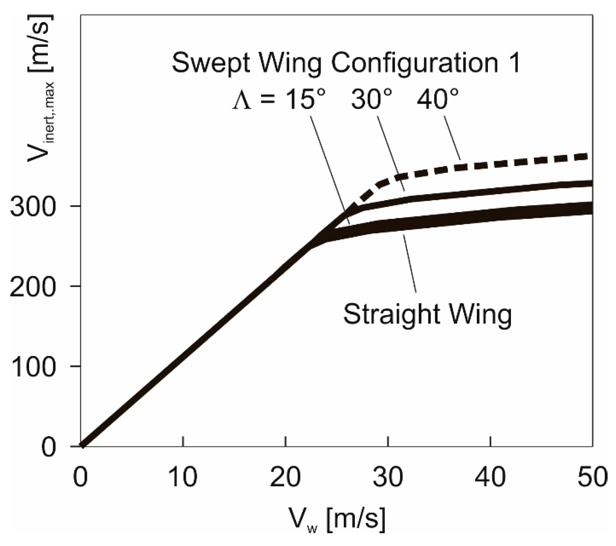
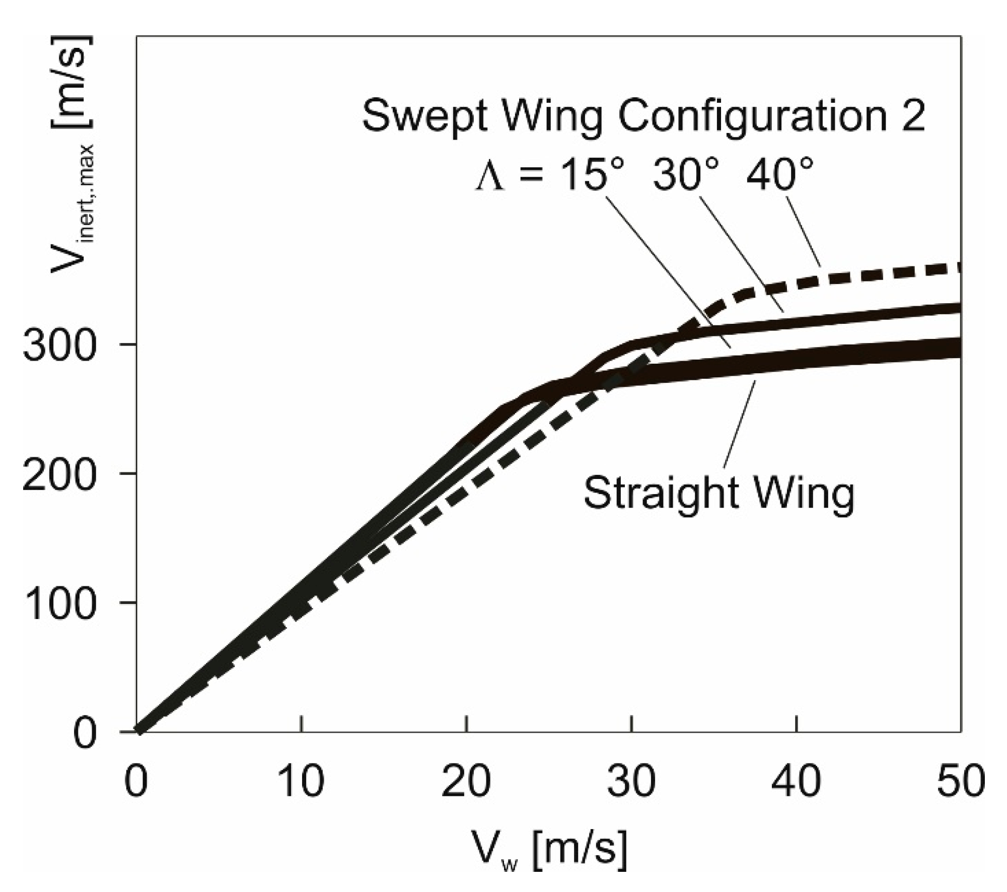
4.3. Potential of Wing Sweep for Enhancing the Maximum-Speed Performance

Based on the results on the validation of the energy model in the previous Chapters, it is assumed that this model is suitable for showing the potential of wing sweep for enhancing the maximum-speed performance. Thus, the maximum speed,   V i n e r t , m a x , can be determined using Equation (20). For this purpose, the maximum lift-to-drag ratio ( C L / C D ) m a x of the wing configuration under consideration is required as the decisive aerodynamic characteristic. On this basis, results and findings on the maximum speed are derived. Results are presented in Figure 15 and Figure 16 which show the maximum speed, V i n e r t , m a x , dependent on the wind speed, V w , for the swept wing configurations 1 and 2 and for the straight wing reference case.
Results for the swept wing configuration 1 are provided by Figure 15 which presents V i n e r t , m a x for three sweep angle cases ( Λ = 15 ° , 30°, 40°) and for the straight wing reference cases. Generally, the four cases show as a characteristic feature of the V i n e r t , m a x curves that there is a left curve part with a large gradient (the same for all cases) that is associated with the incompressible Mach number region and a right curve part with a reduced gradient that is associated with the compressible Mach number region. The right parts of the V i n e r t , m a x curves are of primary interest because the maximum-speed level is highest in these parts for each curve. The relationship between the four V i n e r t , m a x curves shows the effect of wing sweep on the achievable maximum speed.
The main result is that wing sweep yields an enhancement of the maximum-speed performance by increasing, V i n e r t , m a x , when compared with the straight wing reference case. The effect of wing sweep can be rated as follows:
Sweep angles up to around 15° yield only a very small improvement.
The area between the V i n e r t , m a x curve for Λ = 15 ° and the V i n e r t , m a x curve for Λ = 30 ° shows that there are efficient possibilities for enhancing the maximum-speed performance by wing sweep. The area between the V i n e r t , m a x curve for Λ = 30 ° and the V i n e r t , m a x curve for Λ = 40 ° can serve as an indication for the performance potential of larger sweep angles.
For swept wing configuration 2, there is also a possibility of enhancing the maximum-speed performance. This is shown in Figure 16 which presents results on V i n e r t , m a x for swept wing configuration 2. Here, again, it can be distinguished between left and right V i n e r t , m a x curve parts which relate to the incompressible and compressible Mach number regions.
A comparison with swept wing configuration 1 shows that the increase in V i n e r t , m a x is basically smaller. This holds true for the entire V w region. Furthermore, swept wing configuration 2 begins to become effective for increasing V i n e r t , m a x only at higher wind speeds. In addition, swept wing configuration 2 shows smaller V i n e r t , m a x values than the straight wing configuration in the incompressible Mach number region. This is due to the smaller ( C L / C D ) m a x values in that region which are caused by the higher lift-dependent drag resulting from the lower aspect ratio. On the whole, swept wing configuration 2 is a less effective means for enhancing the maximum-speed performance.

5. Further Effects of Wing Sweep Important for High-Speed Dynamic Soaring
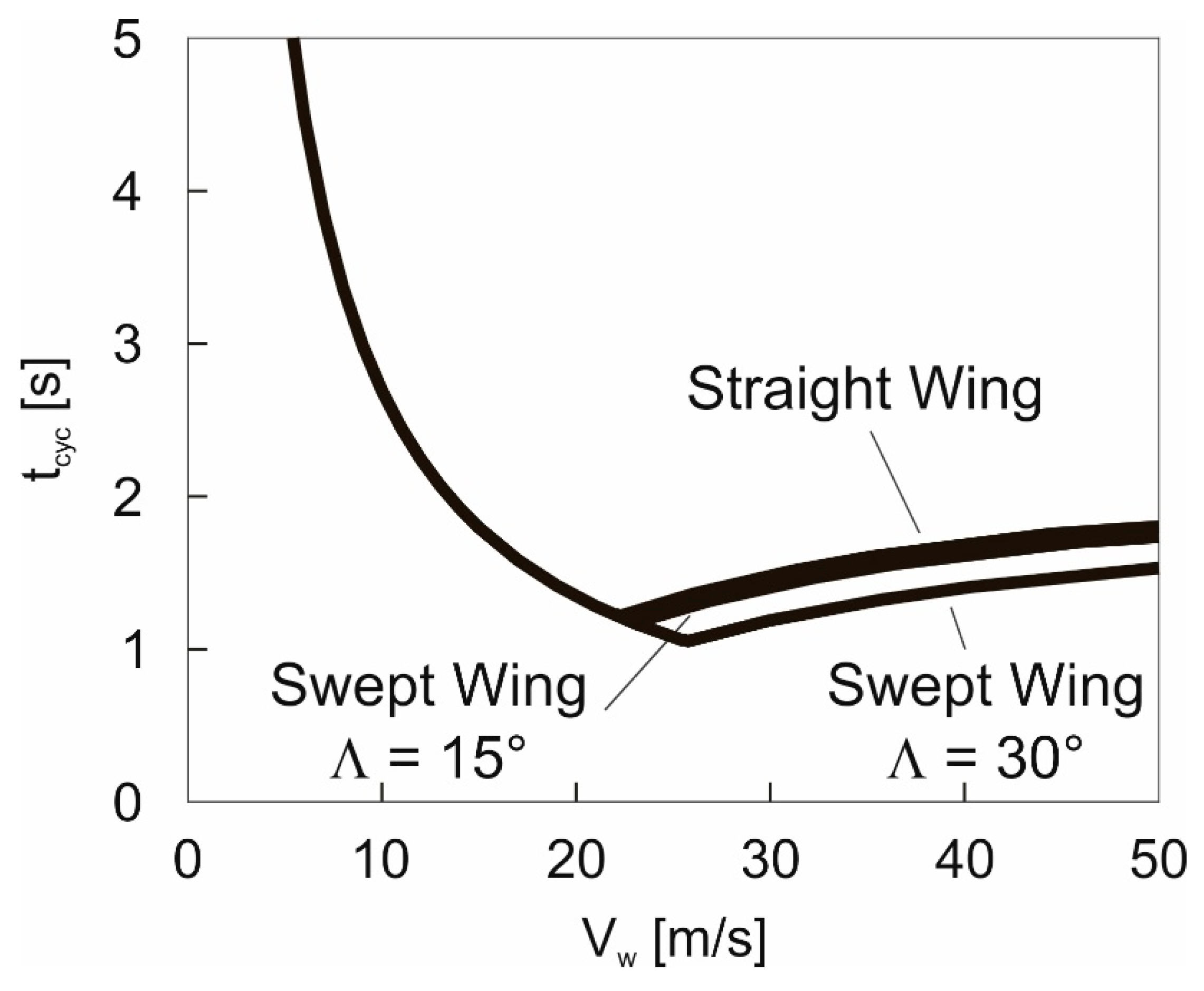
The problems dealt with in the previous Chapter are concerned with the speed performance enhancement achievable with wing sweep. There are other, non-performance topics that are important for high-speed dynamic soaring.
One topic is the controllability of the vehicle or flyability at the extreme speed level which poses unique challenges, associated with short time periods [5,6,8]. Another topic relates to the loads acting on the vehicle which can be extraordinarily large because of rapid turns at extreme speeds possible in high-speed dynamic soaring, manifesting in large load factors [5,6]. A further topic is the air space required for dynamic soaring in terms of the shape and extension of the trajectory. The question is whether there are relationships between these topics and the wing configuration regarding straight or swept wing shapes.
The problems associated with these non-performance topics can be dealt with addressing the following quantities:
cycle time
load factor
trajectory radius
The treatment of the addressed topics in the following Sections is concerned with swept wing configuration 1 as this is the more effective means for enhancing the maximum-speed performance.
The energy model has been validated so that it can be used in lieu of the 3-DOF dynamics model. Thus, the energy model is suitable for analyzing the addressed non-performance topics.

5.1. Optimal Cycle Time
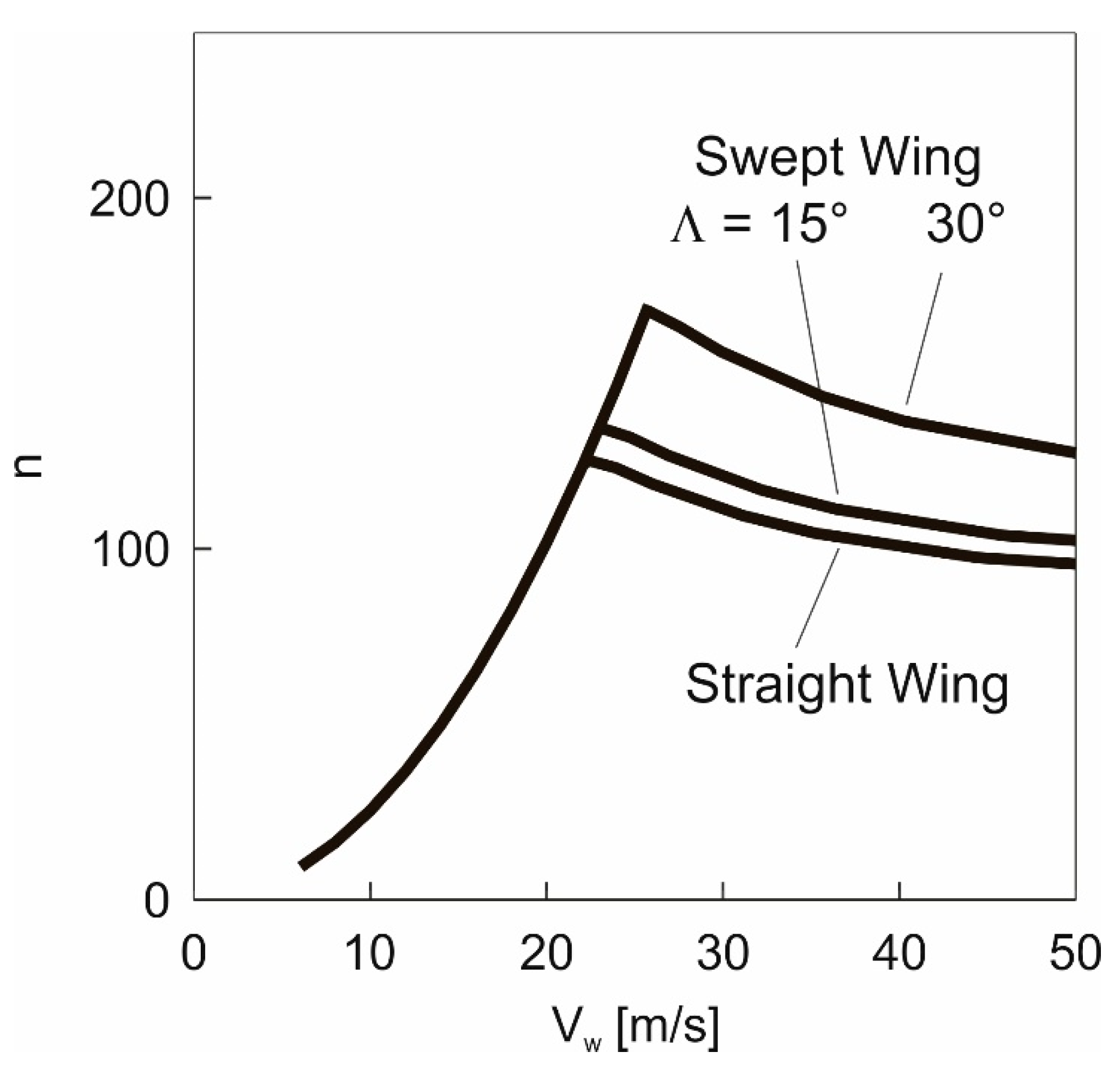
The following expression generally holds true for the time completing a trajectory loop cycle
t c y c = 2 π R c y c V ¯ i n e r t
Applying the load factor relation in curved flight
n = L m g = C L ρ / 2 V ¯ i n e r t 2 S m g
and accounting for Equation (16), the cycle time of a loop in high-speed dynamic soaring can be expressed as
t c y c = 2 π m C L ρ / 2 S V ¯ i n e r t
The optimal loop for achieving the maximum speed V i n e r t , m a x is, according to Equation (20), performed at the maximum lift-to-drag ratio, ( C L / C D ) m a x , and thus at the associated lift coefficient, C L * . Using Equation (19) with γ t r 1 , the optimal cycle time is obtained as
t c y c = 4 π 2 m ρ S 1 C L * ( C L / C D ) m a x V w
This relation describes the effect of wing sweep on t c y c . That effect is due to ( C L / C D ) m a x and C L * since each of them is dependent on wing sweep.
A quantitative insight into the wing sweep effect can be provided examining Equation (32) for the vehicle under consideration. Results are presented in Figure 17 for the swept wing configuration 1 and for the straight wing configuration used as reference. The straight wing reference configuration features a decrease of t c y c in the left curve part which is associated with the incompressible Mach number region (constancy of ( C L / C D ) m a x and C L * ) and an increase in the right curve part which is associated with the compressible region (decrease of ( C L / C D ) m a x and C L * ).
The wing sweep influence on t c y c , Equation (32), manifests in such a way as to shift the beginning of the C L * and ( C L / C D ) m a x decrease to higher Mach numbers. Thus, the wing sweep effect on t c y c begins to becomes effective for swept wing configuration 1 at a correspondingly higher Mach number which in turn is associated with a higher wind speed V w .

5.2. Load Factor

High-speed dynamic soaring involves a rapid flight maneuver that shows a large turning rate and a large inertial speed. Thus, there are high loads acting on the vehicle, to the effect that normal accelerations of an order of magnitude of 100 g are reached [8]. As a result, large loads are typical for high-speed dynamic soaring.
A relation between the load factor, n , and the wind speed, V w , in maximum-speed dynamic soaring can be derived using Equations (19) and (30) to yield
n = 1 2 π 2 ρ S m g C L * C L C D m a x 2 V w 2
This solution shows that the effect of wing sweep on n is relating to ( C L / C D ) m a x and C L * , according to their dependence on wing sweep. The quadratic form of the ( C L / C D ) m a x term in Equation (33) is indicative for an increased influence.
Quantitative results on the effect of wing sweep are provided by Figure 18 which presents n dependent on V w for the swept wing configuration 1 and for the straight wing reference configuration. The straight wing reference configuration shows an increase of n in the left curve part and a decrease in the right curve par, corresponding to the incompressible and compressible Mach number regions and the related behavior of ( C L / C D ) m a x and C L * .
The effect of wing sweep manifests in such a way that there is a difference in terms of larger n values in the compressible Mach number region. This is due to the shift of the beginning of the C L * and ( C L / C D ) m a x decrease to higher Mach numbers resulting from wing sweep.

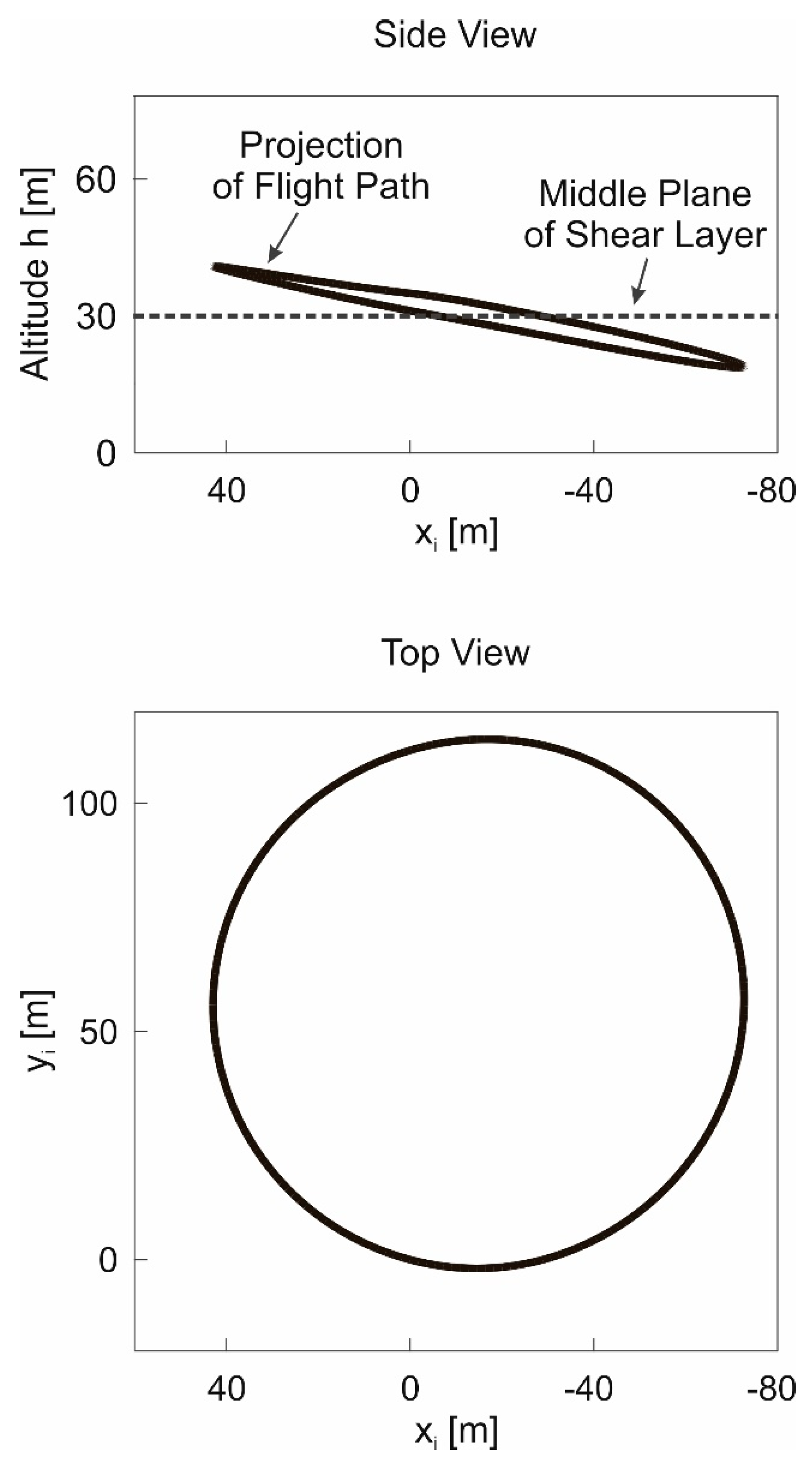
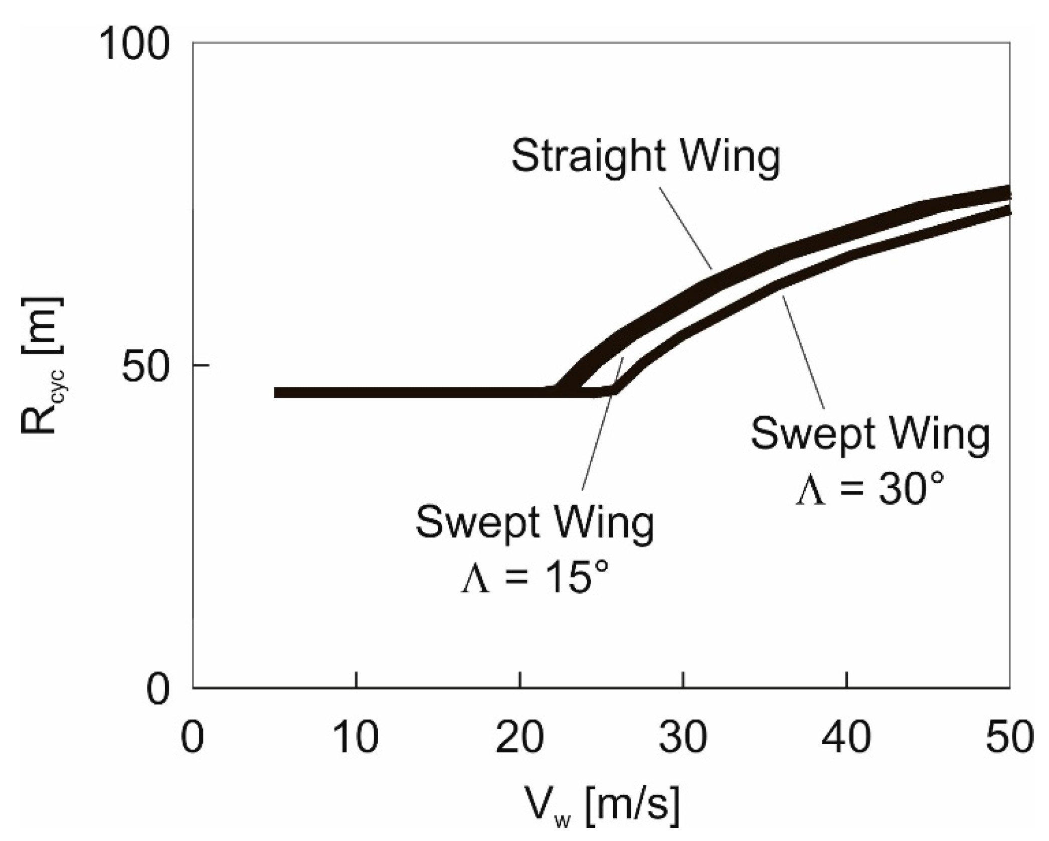
5.3. Trajectory Radius of Maximum-Speed Cycle

The air space required in high-speed dynamic soaring is determined by the shape and extension of the trajectory. In Figure 6, top and side views of an optimized maximum-speed trajectory loop are presented, thus, providing information of the extensions in the longitudinal, lateral and vertical directions. A question is whether the wing configuration in terms of straight or swept wings plays a role regarding the required airspace through its relationship with the maximum speed, V i n e r t , m a x , and the wind speed, V w . The trajectory radius is considered a quantity that can be used to address the air space issue.
With reference to Equations (16) and (30), the radius of the trajectory loop in high-speed dynamic soaring can be expressed as
R c y c = 2 m ρ S 1 C L
Accounting for C L = C L * holding true for the maximum-speed loop, the relation of the optimal trajectory radius is obtained as
R c y c = 2 m ρ S 1 C L *
This relation shows that the effect of wing sweep on R c y c is due to C L * , according to the influence of wing sweep on C L * . A further outcome is that R c y c is not explicitly dependent on V i n e r t , m a x or V w .
A quantitative insight into the wing sweep effect is provided by Figure 19 which presents R c y c dependent on V w for the swept wing configuration 1 and for the straight wing reference configuration. In the left part of the diagram, R c y c is constant and the same for all cases. In the right part of the diagram, R c y c shows an increase. This increase is due to C L * because C L * depends on M a (Figure 5).
The effect of wing sweep yields a difference to the straight wing only in the compressible Mach number region in as much as the increase of R c y c is reduced. This due to the shift in the beginning of the C L * decrease to higher Mach numbers.

6. Conclusions

Dynamic soaring shows a unique flight performance capability by enabling extremely high speeds in shear winds involving a thin layer that separates regions of large and small wind speeds, as they exist at ridges. It is found that the speed level now reached in dynamic soaring approaches the high subsonic Mach number region, with the result that the compressibility-related drag rise causes a limiting effect on the achievable speed performance. Wing sweep is considered as a means for shifting the beginning of the compressibility-related drag rise to higher Mach numbers. For dealing with the related issues, appropriate flight mechanics models are developed and a suitable optimization method is used, with the goal to determine the speed performance enhancement by wing sweep. Analytic solutions are derived for describing the effects of wing sweep. It is shown that small sweep angles have only a minor effect and that larger sweep angles are necessary for achieving a significant improvement. In conclusion, it is possible to enhance the maximum-speed performance in high-speed dynamic soaring by wing sweep.

Author Contributions

Conceptualization, G.S.; methodology, G.S. and B.G.; software, B.G.; validation, G.S., B.G. and H.H.; formal analysis, G.S., B.G. and H.H.; writing—original draft preparation, G.S.; writing—review and editing, G.S., B.G. and H.H. All authors have read and agreed to the published version of the manuscript.

Funding

This research received no external funding.

Institutional Review Board Statement

Not applicable.

Informed Consent Statement

Not applicable.

Data Availability Statement

Not applicable.

Conflicts of Interest

The authors declare no conflict of interest.

Nomenclature

aijcoefficients
bwing span
CDdrag coefficient
CLlift coefficient
Ddrag
Eenergy
gacceleration due to gravity
haltitude
Jperformance criterion
Llift
MaMach number
mmass
nload factor
Rcycloop radius
Swing reference area
slength
ttime
u, v, wispeed components
ucontrol vector
Vaairspeed
Vinertinertial speed
Vwwind speed
xlongitudinal coordinate
xstate vector
Wwork
ylateral coordinate
zvertical coordinate
Aaspect ratio
χazimuth angle
γflight path angle
Λ sweep angle
μbank angle
ρair density

Appendix A. Formulation of Optimal Control Problem

The problem of determining the maximum speed achievable with swept-wing gliders was solved using an optimization method capable of dealing with highly dynamic and unsteady flight maneuvers [20].
The optimization problem is to determine the maximum speed achievable with dynamic soaring. This means to find out the closed-loop dynamic soaring trajectory that shows the maximum speed in the course of the loop. For this purpose, the following performance criterion is specified
J x t = V i n e r t t
For maximizing J x t , the optimal control problem can be formulated as to determine the optimal controls
u * t = [ C ^ L * t , μ a * t ] T
the optimal states
x * t = [ u i * t , v i * t , w i * t , x * t , y * t , h * t ] T
and the associated, optimal cycle time t c y c , subject to the dynamic system according to Equation (1)
x ˙ t = f x t , u t
to control and state constraints
C L , m i n C L C L , m a x
h h m i n
and to periodicity boundary conditions
Ψ x = x t c y c x 0 = 0
The optimal control problem is solved using the direct optimal control tool FALCON.m [27]. To this end, a full discretization of the optimal control problem on the time grid t ¯ is performed, resulting in the discretized states x ¯ and controls u ¯ . The dynamic constraints given by the equations of motion are replaced by a set of defect equations (equality constraints)
c e q , k x ¯ , u ¯ = x ¯ k + 1 x ¯ k t ¯ k + 1 t ¯ k 2 f x ¯ k + 1 , u ¯ k + 1 + f x ¯ k , u ¯ k = 0
at every point on the discretized time grid. These constraints represent a trapezoidal quadrature of the dynamic equations. Furthermore, all path constraints given in Equation (A5), i.e., box constraints on selected control and state variables, are evaluated on this grid, yielding
c i n e q , k x ¯ , u ¯ = C L , m i n C ¯ L , k C ¯ L , k C L , m a x   h m i n h ¯ k 0
for every point t ¯ k on the discretized time grid. Using the above-mentioned discretized approximations of the objective function, differential equations and constraints contained in the original optimal control problem, the Lagrangian function can be constructed for a nonlinear programming (NLP) problem:
L = λ 0 V i n e r t t ¯ f + λ k T c e q , k x ¯ , u ¯ + λ Ψ T Ψ x ¯ + μ k T c i n e q , k x ¯ , u ¯
The optimization software IPOPT [28] is utilized to find the solution of the constructed NLP problem, which employs an interior-point method solving for the (Karush-Kuhn-Tucker) first-order optimality conditions
( optimality ) z L = 0
( feasibility ) λ L = 0
( complementarity ) μ k T c i n e q , k x ¯ , u ¯ + τ = 0
where z represents the primal variables x ¯ , u ¯ , t ¯ f , λ and μ represent dual variables, i.e., the vectors of Lagrange multipliers to equality and inequality constraints, respectively and τ is the barrier parameter, which is driven to zero by the interior-point optimization software. The corresponding function values, gradient and Hessian matrices are supplied to IPOPT by FALCON.m during every iteration. After calculation of an efficient step in the primal and dual variables, IPOPT returns an updated of these variables until Equations (A10)–(A12) are satisfied. The solution of the original optimal control problem can be reconstructed from the solution of the NLP.

References

  1. Idrac, P. Experimentelle Untersuchungen über den Segelflug Mitten im Fluggebiet Großer Segelnder Vögel (Geier, Albatros Usw.)—Ihre Anwendung auf den Segelflug des Menschen; Verlag von R. Oldenbourg: München, Germany; Berlin, Germany, 1932. [Google Scholar]
  2. Cone, C.D., Jr. A mathematical analysis of the dynamic soaring flight of the albatross with ecological interpretations. In Special Scientific Report No. 50; Virginia Institute of Marine Science: Gloucester Point, VA, USA, 1964. [Google Scholar]
  3. Sachs, G. Minimum shear wind strength required for dynamic soaring of albatrosses. Ibis 2005, 147, 1–10. [Google Scholar] [CrossRef]
  4. Wurts, J. Dynamic soaring. SE Modeler Mag. 1998, 5, 2–3. [Google Scholar]
  5. Richardson, P.L. High-speed dynamic soaring. R/C Soar. Dig. 2012, 29, 36–49. [Google Scholar]
  6. Lisenby, S. Dynamic soaring. In Proceedings of the Big Techday 10 Conference, München, Germany, 2 June 2017; TNG Technology Consulting GmbH: Unterföhring, Germany, 2017. [Google Scholar]
  7. Sachs, G.; Grüter, B. Trajectory optimization and analytic solutions for high-speed dynamic soaring. Aerospace 2020, 7, 47. [Google Scholar] [CrossRef] [Green Version]
  8. Richardson, P.L. High-speed robotic albatross: Unmanned aerial vehicle powered by dynamic soaring. R/C Soar. Dig. 2012, 29, 4–18. [Google Scholar]
  9. Sachs, G.; Grüter, B. Dynamic soaring at 600 mph. In Proceedings of the AIAA SciTech 2019 Forum, San Diego, CA, USA, 7–11 January 2019; pp. 1–13. [Google Scholar]
  10. DSKinetic. Available online: www.DSKinetic.com (accessed on 11 August 2021).
  11. Deittert, M.; Richards, A.; Toomer, C.A.; Pipe, A. Engineless unmanned aerial vehicle propulsion by dynamic soaring. J. Guid. Control Dyn. 2009, 32, 1446–1457. [Google Scholar] [CrossRef]
  12. Langelaan, J.W.; Roy, N. Enabling new missions for small robotic aircraft. Science 2009, 326, 1642–1644. [Google Scholar] [CrossRef] [PubMed]
  13. Lawrance, N.R.J.; Acevedo, J.J.; Chung, J.J.; Nguyen, J.L.; Wilson, D.; Sukkarieh, S. Long endurance autonomous flight for unmanned aerial vehicles. AerospaceLab 2014, 8, 1–15. [Google Scholar] [CrossRef]
  14. NASA. Available online: http://www.max3dmodels.com/vdo/NASA-Albatross-Dynamic-Soaring-Open-Ocean-Persistent-Platform-UAV-Concept/F4zEaYl01Uw.html (accessed on 8 April 2020).
  15. Bonnin, V.; Benard, E.; Moschetta, J.M.; Toomer, C.A. Energy-harvesting mechanisms for UAV flight by dynamic soaring. Int. J. Micro Air Veh. 2015, 7, 213–229. [Google Scholar] [CrossRef]
  16. Sachs, G.; Grüter, B. Maximum travel speed performance of albatrosses and UAVs using dynamic soaring. In Proceedings of the AIAA Scitech 2019 Forum, San Diego, CA, USA, 7–11 January 2019. [Google Scholar]
  17. Mir, I.; Maqsood, A.; Taha, H.E.; Eisa, S.A. Soaring energetics for a nature inspired unmanned aerial vehicle. In Proceedings of the AIAA SciTech Forum 2019-1622, San Diego, CA, USA, 7–11 January 2019; pp. 1–11. [Google Scholar] [CrossRef]
  18. Gavrilović, N.; Bronz, M.; Moschetta, J.-M. Bioinspired energy harvesting from atmospheric phenomena for small unmanned aerial vehicles. J. Guid. Control Dyn. 2020, 43, 685–699. [Google Scholar] [CrossRef]
  19. Roskam, J.; Lan, C.-T.E. Airplane Aerodynamics and Performance; DARcorporation: Lawrence, KS, USA, 1997. [Google Scholar]
  20. Sachs, G.; Grüter, B. High-speed flight without an engine: A unique performance capability enabled by dynamic soaring. J. Guid. Control Dyn. 2021, 44, 812–824. [Google Scholar] [CrossRef]
  21. Anderson, J.D., Jr. Fundamentals of Aerodynamics; McGraw-Hill Education: New York, NY, USA, 2017. [Google Scholar]
  22. RCSpeeds. Available online: http://rcspeeds.com (accessed on 12 August 2021).
  23. Schygulla, M. Aerodynamische Auslegung Eines Transsonischen Flugkonzeptes für Dynamic Soaring. Bachelor’s Thesis, Institute of Aerodynamics and Gas Dynamics, University of Stuttgart, Stuttgart, Germany, 2016. [Google Scholar]
  24. Nicolai, L.M.; Carichner, G.E. Fundamentals of Aircraft and Airship Design, Volume I—Aircraft Design; American Institute of Aeronautics and Astronautics, Inc.: Reston, VA, USA, 2010. [Google Scholar]
  25. Rossow, C.-C. Aerodynamik. In Handbuch der Luftfahrzeugtechnik; Carl Hanser Verlag: München, Germany, 2014. [Google Scholar]
  26. Tomas, F. Fundamentals of Sailplane Design; Milgram, J., Ed.; College Park Press: College Park, MD, USA, 1999. [Google Scholar]
  27. Rieck, M.; Bittner, M.; Grüter, B.; Diepolder, J. FALCON.m—User Guide; Institute of Flight System Dynamics, Technische Universität München: München, Germany, 2016. [Google Scholar]
  28. Wächter, A.; Biegler, L.T. On the implementation of an interior-point filter line-search algorithm for large-scale nonlinear programming. Math. Program. 2006, 106, 25–57. [Google Scholar] [CrossRef]
Figure 1. High-speed dynamic soaring trajectory and shear wind scenario at ridge.
Aerospace 08 00229 g001
Figure 2. Speed vectors and inertial coordinate system. (The x axis is chosen parallel to the wind speed vector V w and pointing in the opposite direction).
Aerospace 08 00229 g002
Figure 3. Oblique view on high-speed dynamic soaring loop. (The inclination of the trajectory relative to the horizontal is shown exaggerated for representation purposes).
Aerospace 08 00229 g003
Figure 4. Drag coefficient of straight wing configuration dependent on lift coefficient, C L and Mach number, M a , [7].
Aerospace 08 00229 g004
Figure 5. Maximum lift-to-drag ratio, ( C L / C D ) m a x and associated lift coefficient, C L * , dependent on Mach number, M a , (relating to drag polar in Figure 4.
Aerospace 08 00229 g005
Figure 6. Dynamic soaring loop optimized for maximum speed, V i n e r t , m a x = 271.8   m / s .
Aerospace 08 00229 g006
Figure 7. Side and top views of dynamic soaring loop optimized for maximum speed, V i n e r t , m a x = 271.8   m / s .
Aerospace 08 00229 g007
Figure 8. Time histories of speeds, V i n e r t and V a , and Mach number, M a , of dynamic soaring loop optimized for maximum speed, V i n e r t , m a x = 271.8   m / s .
Aerospace 08 00229 g008
Figure 9. Maximum speed, V i n e r t , m a x , dependent on wind speed, V w .
Aerospace 08 00229 g009
Figure 10. Lift-to-drag ratio in maximum-speed dynamic soaring.   ( C L / C D ) a v : actual lift-to-drag ratio, 3-DOF dynamics model; ( C L / C D ) m a x , a v : maximum lift-to-drag ratio, 3-DOF dynamics model.
Aerospace 08 00229 g010
Figure 11. Maximum speed, V i n e r t , m a x , dependent on wind speed, V w and on maximum lift-to-drag ratio, ( C L / C D ) m a x . Aerospace 08 00229 i001 
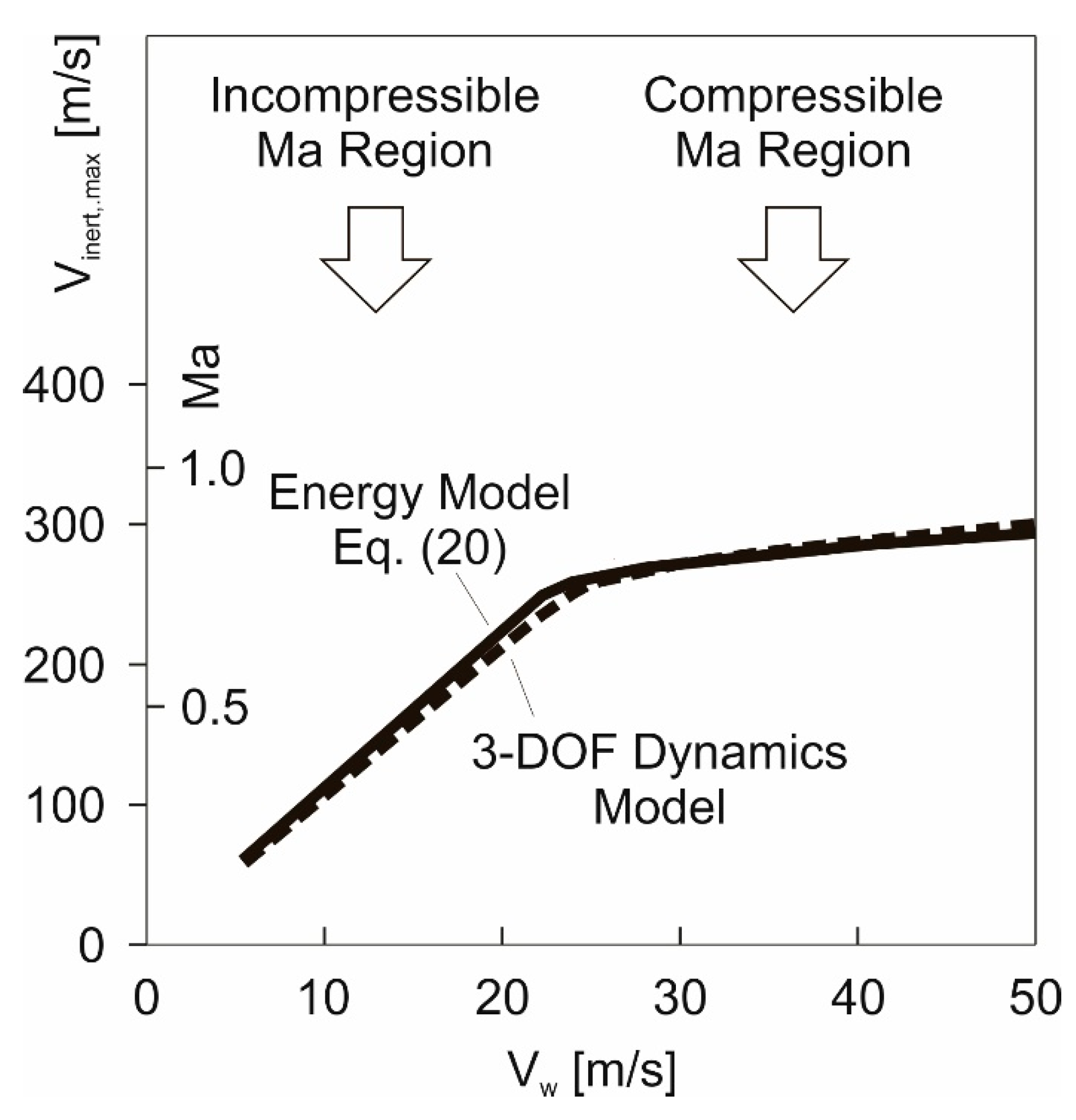
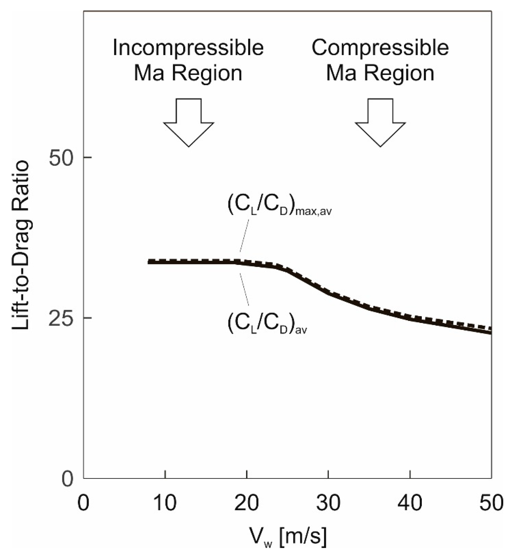
Results obtained using the energy model, Equation (20). Aerospace 08 00229 i002 
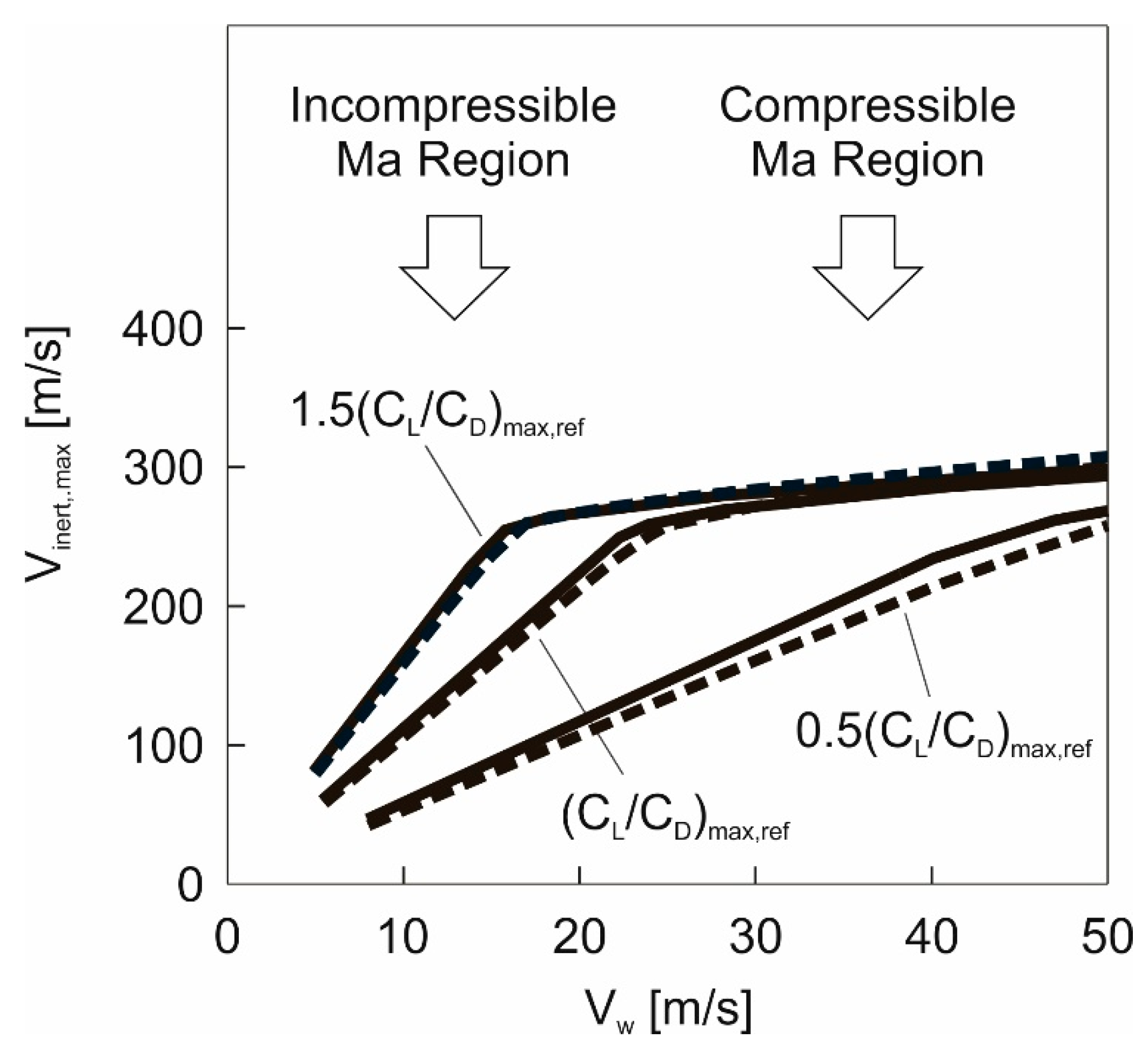
Results obtained using the 3-DOF dynamics model.
Aerospace 08 00229 g011
Figure 12. Effect of Mach number, M a , on lift-to-drag ratio of glider model wings (from [23]).
Aerospace 08 00229 g012
Figure 13. Planform of swept wing configuration used for Figure 12 (from [23]).
Aerospace 08 00229 g013
Figure 14. Swept wing configurations 1 and 2.
Aerospace 08 00229 g014
Figure 15. Effect of wing sweep on maximum speed, V i n e r t , m a x , for swept wing configuration 1.
Aerospace 08 00229 g015
Figure 16. Effect of wing sweep on maximum speed, V i n e r t , m a x , for swept wing configuration 2.
Aerospace 08 00229 g016
Figure 17. Effect of wing sweep on the cycle time for swept wing configuration 1 in maximum-speed dynamic soaring.
Aerospace 08 00229 g017
Figure 18. Effect of wing sweep on the load factor for swept wing configuration 1 in maximum-speed dynamic soaring.
Aerospace 08 00229 g018
Figure 19. Effect of wing sweep on the trajectory radius for swept wing configuration 1 in maximum-speed dynamic soaring.
Aerospace 08 00229 g019
Publisher’s Note: MDPI stays neutral with regard to jurisdictional claims in published maps and institutional affiliations.

