
Neural Nonlinear Autoregressive Model with Exogenous Input (NARX) for Turboshaft Aeroengine Fuel Control Unit Model †


Department of Engineering for Innovation, University of Salento, Via per Monteroni, 73100 Lecce, Italy
*
Author to whom correspondence should be addressed.
†
This paper has been presented in AVT-357 Research Workshop on Technologies for future distributed engine control system (DECS) hosted by the Science and Technology Organization in NATO during 11–13 May 2021.
Aerospace 2021, 8(8), 206; https://doi.org/10.3390/aerospace8080206
Submission received: 8 June 2021
/
Revised: 12 July 2021
/
Accepted: 22 July 2021
/
Published: 29 July 2021
(This article belongs to the Special Issue Technologies for Future Distributed Engine Control Systems)
Abstract
:One of the most important parts of a turboshaft engine, which has a direct impact on the performance of the engine and, as a result, on the performance of the propulsion system, is the engine fuel control system. The traditional engine control system is a sensor-based control method, which uses measurable parameters to control engine performance. In this context, engine component degradation leads to a change in the relationship between the measurable parameters and the engine performance parameters, and thus an increase of control errors. In this work, a nonlinear model predictive control method for turboshaft direct fuel control is implemented to improve engine response ability also in presence of degraded conditions. The control objective of the proposed model is the prediction of the specific fuel consumption directly instead of the measurable parameters. In this way is possible decentralize controller functions and realize an intelligent engine with the development of a distributed control system. Artificial Neural Networks (ANN) are widely used as data-driven models for modelling of complex systems such as aeroengine performance. In this paper, two Nonlinear Autoregressive Neural Networks have been trained to predict the specific fuel consumption for several transient flight maneuvers. The data used for the ANN predictions have been estimated through the Gas Turbine Simulation Program. In particular the first ANN predicts the state variables based on flight conditions and the second one predicts the performance parameter based on the previous predicted variables. The results show a good approximation of the studied variables also in degraded conditions.
1. Introduction
An aeroengine is a multi-parameter, nonlinear, and very complicated thermodynamic system that operates in a highly changeable environment. Furthermore, the performance of its components is generally prone to degradation throughout the course of its life. As a result, it is critical to correctly simulate the engine’s behavior over its entire flight envelope. Finally, it is still more essential to implement an on-board model embedded in Full Authority Digital Electronics Control (FADEC) in order to track in real-time, the information of the engine performance [1]. However, this centralized control system is found to be complex since it receives information from all the sensors installed on the engine, and it requires a complex architecture to meet the complex control requirements [2]. To reduce the degree of complexity of the system, and improve its potential, the centralized control system is transformed into a distributed control system [3] and decentralize the control system into multiple data management systems network. The benefits of this system can be many:
- Increased performance with the reduction in engine weight due to digital signaling, lower wire/connector count, reduced cooling need. 5% increase in thrust-to-weight ratio;
- Improved Mission Success: System availability improvement due to automated fault isolation, reduced maintenance time, and modular line-replaceable unit (LRU). 10% increase in system availability;
- Lower Life Cycle Cost: Reduced cycle time for design and manufacturing; reduced component and maintenance costs.
In a distributed environment, intelligent control system platforms can play the role of a key differentiator in terms of system and software architecture development approach, safety, performance, system integration, engine maintenance, obsolescence management, upgradeability, system reuse, and other lifecycle costs. These developments are then accomplished at lower cost.
If a small fault has not been detected during the flight, it could lead to a bigger fault. Additionally, these bigger faults can lead to high maintenance costs and accidents. During the maintenance phase, the condition of the gas turbine engine is investigated by various tests and measurements [4]. The conventional maintenance strategy is TBM (Time Based Maintenance), which divides maintenance work into routine maintenance and different levels of periodical overhaul [5]. The time prescheduled manner is used, basically regardless of the health condition of the machine. This strategy, with good operability, will cause excessive maintenance or fault before the next prescheduled overhaul. The solution of these problems is to adopt CBM (Condition-based maintenance) [6].
Condition-based maintenance (CBM) is performed to provide effective and efficient maintenance in today’s maintenance services.
Monitoring of the parameters makes it possible to calculate parameters of power machine and describe the health condition of machine. With this strategy, the deteriorated equipment works with different performance parameters from new equipment. To guarantee the availability of the machine, predicting the performance degradation trend is a necessary part of reliable maintenance for power machinery. There are many researchers focusing on intelligent maintenance system development based on prognosis [7,8]. The time of replacement can be determined with a prognostic model to guarantee availability and reduce costs. Thus, maintenance costs will decrease and technical staff can have adequate time to prepare for maintenance.
The maintenance theme is chosen because, as also explained in [9], fleet maintenance is very costly and improvements in maintenance logistics, reductions in unscheduled events (and their consequences), and improvements in operational efficiency can have an enormous impact on reducing costs. In this way is possible to develop an integrated approach of iterative algorithms based on Artificial Intelligence to define removal plan and its maintenance work, optimizing engine availability at the customer and maintenance costs.
Turbine engines of the future are more complex and require smart sensors, smart actuators, constant monitoring, and require capability for rapidly processing many parameters. The analysis of the applicability of the distributed architecture in terms of the controls and communication issues and examination of the potential benefits and challenges for implementing distributed FADEC systems.
The control design of aeroengine systems has been investigated in [10] by using distributed architecture and its delay due to the network transmission. The results showed that the designed controller is stable and ensure the desired performance of the aeroengine in the presence of persistent delay.
In order to obtain and analyze as much data as possible, the engine performance simulations have been widely used in gas turbine designs; in this way is possible to decrease design and development costs [11,12,13]. These types of simulations can be classified into design point, off-design steady state, and transient performance simulations based on the engine’s operation. Transient performance simulations are very useful in the initial stage of engine design. For example, transient data may be used to determine the safety of new engines, including accelerations and decelerations, and to offer a numerical test-bed for control system development, including the investigation of dynamics behavior and interaction between engines and control systems. Furthermore, the engine is subjected to overloads and over-temperature during transient operations. As a result, these simulations are critical for diagnosing and prognosticating the system’s health.
Furthermore, novel control systems will incorporate real-time prognostics and health monitors to detect degradation of engine performance and failures of its components.
Advanced aircraft control systems will integrate more versatile controllers, which will accomplish the complex task of real-time engine supervision and control combined with engine health management models. The main issue of these intelligent systems is to improve the efficiency of engine components through active control, advanced diagnostics, and prognostics to enhance component performance and life.
Model-based and data-driven techniques are the two primary types of performance simulations and prognosis methods [14,15]. Model-based approaches require a mathematical and physical model of the engine, whereas data-driven methods use recorded or real-time data from sensor measurements to forecast the status of the engine’s components in the future. Because developing a thorough and precise mathematical model of an aeroengine is challenging, data-driven approaches are gaining popularity in the aeroengine community. They represent and simulate the performance of the components and forecast the system’s transient behavior using real or estimated data [16]. In the recent past, machine learning techniques strongly entered the aerospace field due to their flexibility and capacity to analyses and generalize huge amounts of data.
When one considers the vast number of characteristics and variables that may be measured during the functioning of an aircraft engine, it’s easy to see how these approaches can help with the study of such complicated systems. Artificial Neural Networks (ANN) have been widely utilized as a data-driven model for aeroengine performance modeling and simulation. Function Fitting, Nonlinear Input-Output (NIO), Nonlinear AutoRegressive eXogenous (NARX), Long Short-Term Memory (LSTM), Adaptive Network-based Fuzzy Inference System (ANFIS), Feedforward Multi-Layer Perceptron (MLP), Backpropagation Neural Networks (BPNN), and Radial Basis Function (RBF) are all examples of ANN techniques. The authors have demonstrated their capacity to capture the dynamics of complex systems such as gas turbines in [17]. In addition to neural networks, new techniques of Genetic Programming (GP) are also starting to be used in the aerospace sector.
In [18] a model based diagnostic method using Neural Network algorithms has been proposed for fault identification on a turboshaft engine. The Neural Network system can detect the faulted components including the fault pattern and quantity of the engine at various operating conditions.
These machine learning techniques will be treated and used in this work to calculate and predict the evolution of the engine status, in particular the Specific Fuel Consumption (SFC). In this way is possible to find a correlation between each input and output as the Aeroengine is a typical multi-variable model and it is possible to improve the stability of control system.
2. Materials and Methods
2.1. Gas Turbine Modelling
The propulsion system, PW200 Pratt & Whitney Canada, is a family two spool turboshaft engines developed specifically for helicopter applications. This propulsion is a lightweight turboshaft engine with a free turbine (Low Pressure Turbine (LPT)), connected to the rotor shaft with a nominal speed of 6000 rpm, and a single stage centrifugal compressor driven by a single stage turbine (High Pressure Turbine (HPT)). This engine is installed on one of Airbus’ most successful light aircraft, the H135, which is known for its endurance, compact build, low sound levels, reliability, versatility, and cost-competitiveness. The specifications for the PW200 are reported in Table 1.
The data used for this work have been estimated through the Gas Turbine Simulation Program (GSP) and, due to the lack of experimental data, it was not possible to accurately validate the model. GSP is an off-line component-based modelling environment for both aircraft and industrial gas turbines. Gas turbine performance calculations are currently performed using computer software and advanced model-based diagnostic techniques that enable component condition estimation without the need for engine disassembly. Both transient and steady state simulation of any kind of gas turbine configuration can be achieved by establishing a specific arrangement of engine component models.
2.1.1. Design Point
GSP is a powerful tool for performance prediction, emissions calculation, control system design, diagnostics, and off-design analysis. It is especially suitable for sensitivity analysis of some variables such as ambient conditions, component deterioration, and exhaust gas emissions. More information on this software can be found in the GSP11 user manual [19].
The study and investigation of an engine’s design point is the initial stage in constructing an engine model. Figure 1 shows the model created in GSP for the PW200 engine series. Two additional components named Duct are shown in addition to the conventional components (such as turbomachinery, combustion chamber, and nozzles). They are utilized in transient models to add dynamics and volumetric effects, as well as to do mass balance calculations (ICV-Intercomponent Volume method [20,21,22,23]). They have no effect on engine performance and operational characteristics during steady-state conditions.
The design point is given by sea level condition (altitude of 0 m and temperature of 288.15 K), so it is possible to obtain the maximum power. The main design parameters have been reported in Table 2. Iterative modifications were made to the air flow rate and the fuel flow rate injected into the combustion chamber in order to obtain the same power indicated on the specifications. The default compressor and turbine maps were scaled according to a set of input parameters taken from the database of the reference engine. The iteration allowed a prediction of the design take-off power with an accuracy of 1% with respect of the reference engine.
2.1.2. Transient Simulations
All engine characteristics are balanced under stable circumstances, and there is no change in flow qualities at any location in space or in engine parameters over time (speed, temperatures, and compression and expansion ratios). Real engines, on the other hand, can only theoretically achieve a steady state since they undergo significant changes in operating conditions during their operation. All of these modifications cause the engine’s operating point to shift from its initial equilibrium to a new operating point where the engine parameters achieve a new state of equilibrium [21]. Dynamic response refers to the process through which the engine’s operating point shifts from one thermodynamic equilibrium condition to another, and engine performance is transitory.
GSP may also do transient simulations, allowing the user to account for dynamic phenomena such as spool inertia, heat transfer in turbomachinery, and volumetric effects.
To describe the dynamic behavior of the system, power level angle (PLA) changes are performed with standard step, ramp, and pulse signals in different flight conditions from idle to full and vice versa (Figure 2 and Table 3).
Therefore, the data sets used in this work have been simulated during several changes and cover the whole operating range of the engine.
The time series data sets considered are compressor pressure ratio, compressor rotational speed, inlet turbine temperature, fuel flow rate, and specific fuel consumption, based on flight altitude, Mach, and the PLA.
2.1.3. Deteriorated Model
During its life cycle, the engine can suffer several issues due to over-temperatures, erosion of compressor and turbine blades, fouling, bird strikes, etc.
Typically, any fault in a single component or inconsistency in the performance of a group of components can increase machine degradation. To perform fault identification or to create a model for simulating faults, the relationship between physical faults and component deterioration must be determined.
In the fault identification process, it is useful to find a relationship between the faults and their corresponding effects on the engine performance. Table 4 summarizes some of the issues that it is possible to find in the compressor and the turbine and their related effects, where is the compressor mass flow rate, is the compressor efficiency, is the turbine mass flow rate, and is the turbine efficiency.
An issue in the study of engine component degradation is to select the appropriate measured parameters that can reflect the performance degradation of aeroengine to realize its performance degradation forecast [21,22,23]. Thus, exhaust gas temperature (EGT) is often used for engine control, condition monitoring, fault diagnosis, and maintenance decisions. When other conditions remain the same, the higher the EGT is, the more serious the performance degradation of aeroengine is [21,22,23]. However, in this work specific fuel consumption (SFC), compressor pressure ratio, compressor rotational speed, fuel flow, turbine inlet temperature were compared with the corresponding clean and healthy parameters.
GSP allows us to represent the deterioration of the engine in a number of ways. The most used is to run a simulation with a constant degree of deterioration, i.e., a constant decrease of the efficiency and mass flow rate in the case of the compressor. As seen before, this can be represented by the fouling index or the erosion index. Obviously, it is implied that, in this case, the engine considered is already damaged by some of the phenomena seen before. However, in order to make the study as general as possible, a step change has been considered, represented as a variation of the only compressor efficiency. It has been decreased of the 10% with respect to the healthy condition.
2.2. Neural Network Application to Transient Simulations
A neural network is a system that is modeled after the design of organic nerve systems. It is made up of linked neurons arranged in a layering system that includes an input layer, one or more intermediate hidden layers, and an output layer. A feed-forward neural network with one hidden layer is presented as an example in Figure 3. In general, there can be multiple hidden layers. Each node in the layer is a neuron, which can be thought of as the basic processing unit of a neural network.
The input layer is utilized to give varying intensities and strengths of input data. The input signal is received by the input neurons, where it is combined to produce a net input to another neuron. Weight and bias associated with connections among neurons are used to compute the output layer, which has the same number of neurons as the predicted outputs. This is the layer that generates the forecasts. The input and output layers are linked to the intermediate layers. The signals from all the neurons in the preceding layer are received by each neuron in the hidden and output layers, which then compute a weighted sum on the inputs.
An Artificial Neuron is the basic unit of a neural network. It calculates the weighted sum of its inputs and then applies an activation function to normalize the sum. The activation functions can be linear or nonlinear. Additionally, there are weights associated with each input of a neuron. These are the parameters that the network has to learn during the training phase. A schematic diagram if a neuron is shown in Figure 4.
NARX Neural Network
NARX is the most promising technique among ANN-based models for predicting transient behavior of aeroengines. These neural networks are ideally suited to capture the dynamics of complex systems like gas turbines; thus, they may be used for gas turbine design optimization as well as the entire operation and maintenance activities of the aeroengine.
A good approach to dealing with chaotic time series with a large amount of data is one based upon “Nonlinear Autoregressive models with eXogenous input (NARX model)”. The structure of the neural network can be assumed as a “black-box” with the x(t) series at the input and the y(t) series at the output, which is the variable that ANN should predict. This is a powerful class of models that has been demonstrated as well suited for modelling nonlinear systems and especially time series and also the values of the series in the past time.
Learning of NARX networks is more effective than in other neural networks and these networks converge much faster and generalize better than other networks. NARX are recurrent dynamic networks that correlate the current value assumed by the output parameters y(t) in a time series to the past values of the same parameters and of the driving parameters. Thus, this network allows us to use as an input not only the series x(t) but also the values of the series y(t) in the past times. The fundamental equation of the NARX model is as follows:
where d is a parameter called delay.
Neuron’s number in the hidden layer and the delay d can greatly influence both the network training time and its accuracy. The training samples are passed through the network and the output obtained from the network is compared with the actual output. This error is used to change the weights of the neurons such that the error decreases gradually. This is done using the Backpropagation algorithm, also called backprop. It iteratively passes batches of data through the network and updates the weights, so that the error is decreased, and is known as Stochastic Gradient Descent (SGD). The amount by which the weights are changed is determined by a parameter called Learning rate.
In this work, the MATLAB Neural Network tool has been used to build the NARX models for a combination of the simulated time-series data sets of the several flight conditions. The aim of this study is not only to predict the output variables value in future instants of time, but to derive a relationship between the inputs provided to the neural network and the desired output. The Closed-loop structure of the NARX model is shown in Figure 5.
In this work two neural networks have been applied. The first one uses the inputs of ambient conditions (P1, T1), Mach number (M), and power level angle (PLA) and gives as outputs a prediction of fuel flow rate, compressor speed, turbine inlet temperature, and compressor pressure ratio. Then, these variables are used in the second network as an input, together again with ambient condition and Mach number, in order to predict engine performance parameters, i.e., specific fuel consumption (Figure 6).
For each neural network the data need to be divided randomly into training (70%), validation (25%), and test (5%) sets. The validation set was used to ensure that there was no overfitting in the final results. The prediction has been performed for all the simulated cases, but the data have been divided in training and testing data as follows:
In this way, the data to be used for the prediction of the output variables are formed by concatenating the GSP results.
To run the NARX networks, it was decided to use, as training dataset, the PLA signal in Figure 7a calculated in transient conditions with GSP the ambient conditions and Mach depicted in Figure 7a. Each model was trained by using the Bayesian regularization back-propagation functions as the training function, a delay parameter from 1 to 2 was assumed at the input in order to make good (improve) predictions performance and prevent overfitting. The number of neurons in the hidden layer was set equal 10. The neural networks were evaluated and validated after they had been trained, with the PLA shown in Figure 7b, the ambient conditions, and Mach displayed in Figure 7b as inputs. The prediction is one-step-ahead, which means that the network predicts the value of the performance parameters at time t + 1 based on the values of the inputs at prior times.
The parameters used for the comparison of the simulated data YGSP to the predictions of NARX models YNN, are:
- Mean-Square-Error (MSE) defined as follows:
- The Root-Mean-Square-Error (RMSE) defined as follows:
- The coefficient of determination R2 is defined as follows:where n is the number of data of each data set.
Figure 8 represents the training loss curves for performance parameter SFC for the dataset reported in Figure 7. The training loss indicates how well the model is fitting the training data, and how well the model fits new data. It is possible to note that the training loss also goes down over time, achieving low error values for subsequent iterations. The test curve also quickly reaches its lowest value but is slightly higher than the training curve.
3. Results
In order to determine the correct operation of an aircraft engine and evaluate its health condition, it was decided to study the behavior of its main performance parameters in different flight conditions.
Therefore, to understand if the engine has malfunctions or anomalies during its flight conditions, it was decided to use the SFC, as one of the main parameters to be estimated one-step-ahead by the ANNs technique.
The parameters selected as input in NARX models and were considered to have a correlation with the above performance parameters are:
- Engine parameters: shaft speed (Nc), turbine inlet total temperature (TIT), fuel mass flow rate (Wf_b), and compressor pressure ratio (PRc);
- Environment parameters: Mach number (M), atmospheric total temperature (TT1), and total pressure (PT1).
3.1. NARX Neural Networks Prediction Results
3.1.1. Healthy Results
Figure 9 reports the results of the training and testing phase in terms of RMSE and R2 for the datasets reported in Figure 7.
The low RMSE indicates that the neural network approximates well the observed data for both training and test phases. The confirmation of the correct prediction of the observed variable is given also from R2. Its value is close to 1, it indicates a good predictive power of the network.
In the following figures, it is possible to note how the NARX predicts the behavior of the observed variable, obtained from the simulation in GSP, in the training and test phases. At the different neural networks an index has been assigned depending on the variable to be predicted (i.e., NARX1 for prediction of Wf_b).
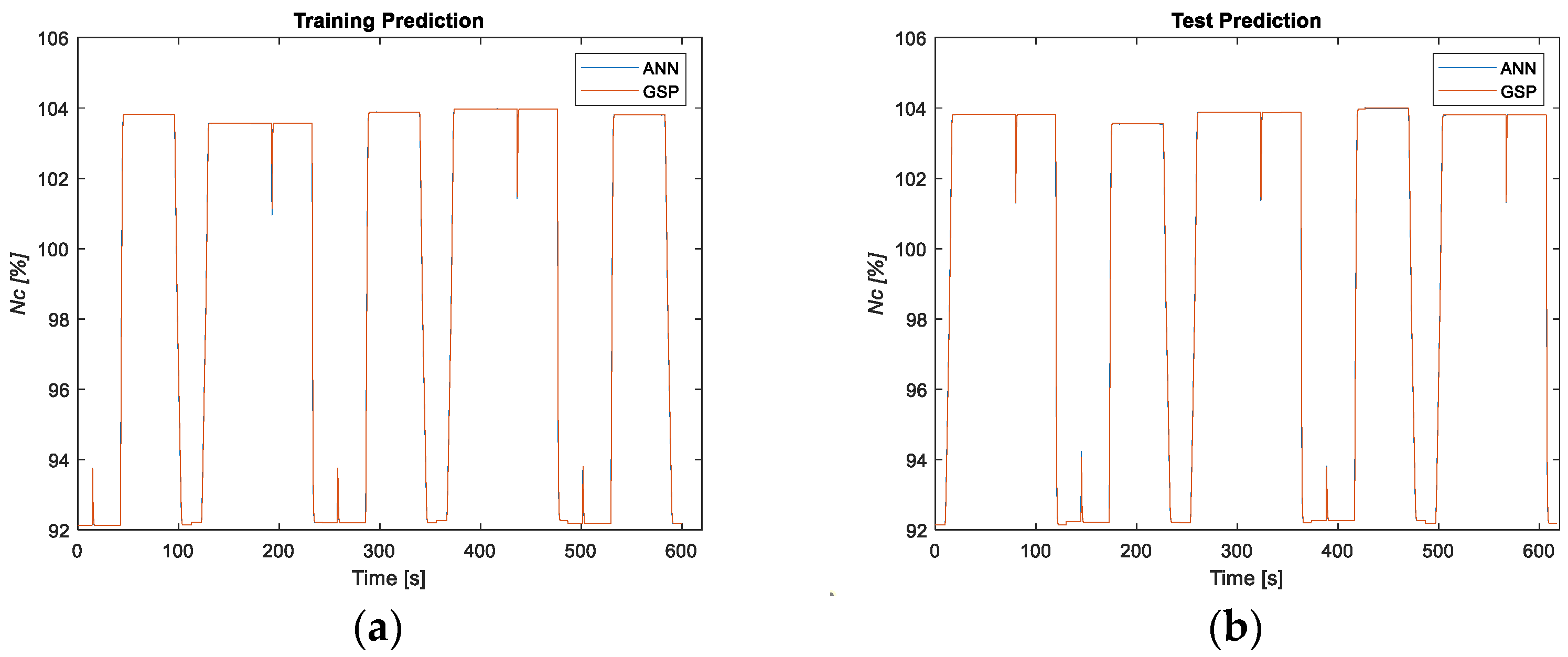
As can be seen from Figure 10, Figure 11, Figure 12, Figure 13, Figure 14, Figure 15, Figure 16 and Figure 17, the neural networks (NARX1, NARX2, NARX3, and NARX4), useful for the prediction of the first set of the state measurable variables, successfully forecast the different variables.
In fact, there is a good approximation for Nc, PRc with a low RMSE, 0, 1 and, respectively. While for the variables Wf_b and TIT the RMSE increase 3, 7 and 1, 4, respectively. For these two variables, it is possible to note a higher percentage of error.
In conclusion, it was observed that NARX can effectively learn complex sequences, passing from different conditions even if these conditions do not occur in real conditions of flight. Please note that the data has been concatenated without taking into account a real transit between the different configurations. It possible to note from Figure 18 a slight difference between the GSP value and the value predicted by the NARX5. These errors, e.g., in Figure 19, appear to have high but still very short peaks; it has been verified that these peaks coincide with the rapid adjustment performed by the PLA, which leads to a rapid change of the fuel flow causing a rapid variation in the observed variables. In such situations, the neural network cannot accurately predict the instantaneous variation, producing high picks and high errors, due to a very short time delay in the prediction. However, when the PLA inputs “were not aggressive”, the engine remained in steady-state conditions and the neural network is able to predict the output variables accurately (Figure 20).
3.1.2. NARX Neural Networks Prediction Results Degraded Model
Data generated from an engine model in the presence of compressor degradation, represented as a variation of 10% of its efficiency with respect to the clean case, were finally used to train and test the adaptive neural network implemented to predict SFC in degraded conditions.
First of all, the ANNs previously implemented and validated without deterioration (clean case) were used to predict the performance with compressor deterioration. It is possible to note from Figure 21 that by using the network previously obtained in the clean case, without adapting to the new degraded conditions, it is not possible to accurately forecast the specific target SFC in degraded conditions.
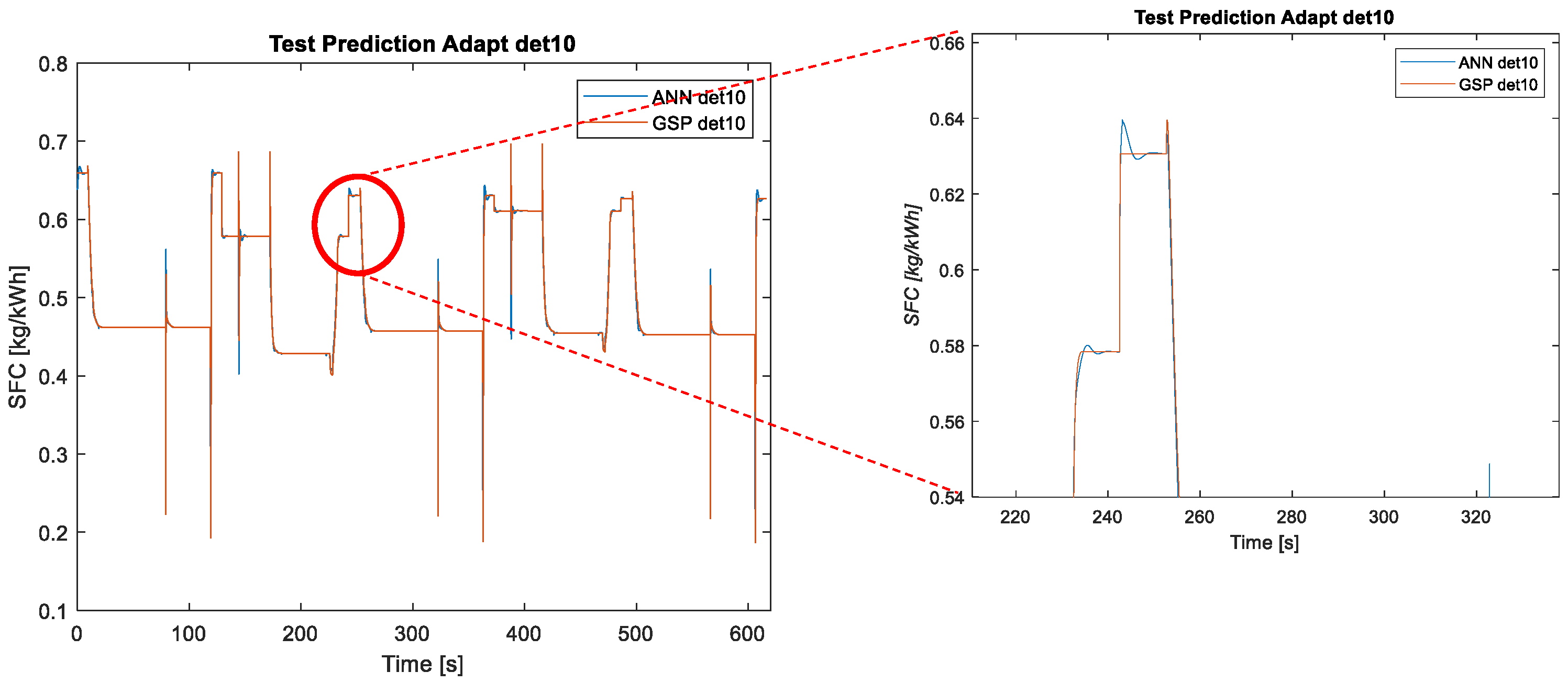
However, by applying the adaptation function, it is possible to improve the prediction of SFC reported in Figure 22. Therefore, an improvement in the variable to be predicted by the adapted network has been achieved, as it is evident from the plot of the error that it is shown in Figure 23. In fact, the average relative error decreases from 1% to 0.4% with both training and test data using the adapted network. The adaptation procedure consists of updating the weights and bias of the network, previously obtained without deterioration. This network can be trained with the adaptive function to produce a particular output sequence. The new network returns the final weights, bias, and new output, and in this section shows degraded performance. It is possible to adapt the network by adding steps in its sequence to get the output even closer to the desired values. This function simulates the network on the input, while adjusting its weights and biases after each timestep in response to how closely its output matches the target.
It is possible to note, in Figure 24, how this function simulates the network on the input, while adjusting its weights and biases after each time-step in response to how closely its output matches the target in order to minimizes the mean square error.
The diagnostic methodology was implemented to predict engine performance degradation using the values of SFC assumed in each degraded engine condition and the ones in a healthy engine. Hence, the training and test of the neural network were done using inputs that describe the flight conditions of the healthy engine connected to the degraded case.
4. Discussion
The main aim of this research was to investigate the dynamic behavior of a turboshaft engine in healthy and degraded conditions during transient phase. In order to create a data set, a 0-D model of the engine was developed using GSP software. The design parameters of each engine component were defined based on the datasheet; once the design point was fixed, the model was validated both in steady and transient conditions. The error of the 0-D model was very low, less than 1% in the case of the SFC. After the validation at the design point, a series of PLA adjustments were simulated by changing the power level angle PLA in different flight conditions, in terms of altitude and Mach. These PLA adjustments, were then concatenated to serve as input for Neural Network model. An artificial Neural Network has been used for the prediction of the performance parameter of the engine with one-step ahead prediction, called Nonlinear AutoRegressive with eXogenous inputs (NARX) neural network.
In this work two neural networks have been applied. The first one uses as inputs the ambient conditions, Mach number, and PLA and gives as output a prediction of fuel flow rate, compressor rotational speed, turbine inlet temperature, and compressor pressure ratio. Then, these variables are used in the second network as an input, together again with ambient conditions and Mach number, in order to predict engine performance parameters, in this case specific fuel consumption. The ability of these two neural networks to learn and predict engine performance in both healthy and damaged situations has been proven. Neural networks have shown to be highly successful models; the training phase becomes so effective, owing to the recurrent usage of parameter values recorded in the previous time instant, that the predictions are great even with a different time series. The results reveal a 98% correlation between real and projected values for all parameters observed for different input signal sequences. In order to maintain the same correlation for a degraded system and in particular a reduction of compressor efficiency, the network needs an adaptation to the new conditions. In this way, it is possible to improve the prediction reducing the overall average error between an un-adapted network and an adapted network. The ability to forecast and know a parameter’s value in the near future is crucial for the creation of an engine control system that can perform engine corrections ahead of time. It is apparent that by converting from a one-step-ahead to a multi-step-ahead approach and attempting to create an SFC prediction for a longer time interval, this forecast may be improved.
In the future, it will be possible to assign as target values, a degradation index or a health indicator and understand if the engine has malfunctions or anomalies during its flight conditions and subsequently estimate its Remaining Useful Life. Furthermore, it is possible to create a neuro control design decentralized for each performance parameter. The input to the existing controller is the training input to the network and the controller output serves as the target. The training must be conducted during the operation. The neural network needs the instantaneous error between the set-point and the process output to train a neural network with a series of those errors and/or the controller outputs in the previous time steps. The inputs and the outputs of the process are replaced with feedback errors and controller outputs.
Author Contributions
Conceptualization, M.G.D.G., L.S., and A.F.; methodology, M.G.D.G., L.S., and A.F.; software, M.G.D.G. and L.S.; investigation, M.G.D.G. and L.S.; writing—original draft preparation, M.G.D.G. and L.S.; writing—review and editing, M.G.D.G. and L.S.; project administration, A.F.; funding acquisition, A.F. All authors have read and agreed to the published version of the manuscript.
Funding
This research was funded by Italian ministry of university and research, project PON “Further”, code ARS01_01283” and “The APC was funded by Italian ministry of university and research”.
Institutional Review Board Statement
Not applicable.
Informed Consent Statement
Not applicable.
Conflicts of Interest
The authors declare no conflict of interest. The funders had no role in the design of the study; in the collection, analyses, or interpretation of data; in the writing of the manuscript, or in the decision to publish the results.
References
- Zheng, Q.; Zhang, H.; Li, Y.; Hu, Z. Aero-Engine On-Board Dynamic Adaptive MGD Neural Network Model within a Large Flight Envelope. IEEE Access 2018, 6, 45755–45761. [Google Scholar] [CrossRef]
- Chen, Y.; Guo, Y.; Li, R. State Feedback Control for Partially Distributed Turboshaft Engine with Time Delay and Packet Dropouts. In Proceedings of the 37th Chinese Control Conference, Wuhan, China, 25–27 July 2018; pp. 25–27. [Google Scholar]
- Timothy, M.S.; Qwen, B.M.; Alireza, R.B.; Fouad, K. Development of Distributed Control Systems for Aircraft Turbo-Fan Engines. In Proceedings of the 52nd AIAA/SAE/ASEE Joint Propulsion Conference, AIAA Propulsion and Energy Forum, American Institute of Aeronautics and Astronautics, Salt Lake City, UT, USA, 25–27 July 2016. [Google Scholar]
- Lee, S.M.; Roh, T.S.; Choi, D.W. Defect diagnostics of SUAV gas turbine engine using hybrid SVM-artificial neural network method. J. Mech. Sci. Technol. 2009, 23, 559–568. [Google Scholar] [CrossRef]
- Xia, T.; Xi, L.; Zhou, X. Modeling and optimizing maintenance schedule for energy systems subject to degradation. Comput. Ind. Eng. 2012, 63, 607.e14. [Google Scholar] [CrossRef]
- Li, Y.G.; Nilkitsaranont, P. Gas turbine performance prognostic for condition based maintenance. Appl. Energy 2009, 86, 2152–2161. [Google Scholar] [CrossRef]
- Biagetti, T.; Sciubba, E. Automatic diagnostics and prognostics of energy conversion processes via knowledge-based systems. Energy 2004, 29, 2553–2572. [Google Scholar] [CrossRef]
- Silva, J.A.M.; Venturini, O.J.; Lora, E.E.S.; Pinho, A.F.; Santos, J.J.C.S. Thermodynamic information system for diagnosis and prognosis of power plant operation condition. Energy 2011, 36, 4072–4079. [Google Scholar] [CrossRef]
- Volponi, A.J. Gas Turbine Engine Health Management Past, Present and Future Trends. In Proceedings of the ASME Turbo Expo 2013: Turbine Technical Conference and Exposition, San Antonio, TX, USA, 3–7 June 2013. [Google Scholar]
- Wang, X.-Y.; Du, X.; Wang, X.-F.; Sun, X.-M.; Li, Y.-S. Controller Design of Aero-engines under the Distributed Architecture with Time Delays. In Proceedings of the 2020 39th Chinese Control Conference (CCC), Shenyang, China, 27–29 July 2020; pp. 6881–6886. [Google Scholar] [CrossRef]
- De Giorgi, M.G.; Campilongo, S.; Ficarella, A. A diagnostics tool for aero-engines health monitoring using machine learning technique. Energy Procedia 2018, 148, 860–867. [Google Scholar] [CrossRef]
- De Giorgi, M.G.; Ficarella, A.; De Carlo, L. Jet engine degradation prognostic using artificial neural networks. Aircr. Eng. Aerosp. Technol. 2019, 92, 296–303. [Google Scholar] [CrossRef]
- Wang, C.; Li, Y.G.; Yang, B.Y. Transient performance simulation of aircraft engine integrated with fuel and control systems. Appl. Therm. Eng. 2017, 114, 1029–1037. [Google Scholar] [CrossRef] [Green Version]
- Kordestani, M.; Saif, M.; Orchard, M.E.; Razavi-Far, R.; Khorasani, K. Failure Prognosis and Applications—A Survey of Recent Literature. IEEE Trans. Reliab. 2021, 70, 728–748. [Google Scholar] [CrossRef]
- Tsoumakas, G.; Katakis, I. Multi-Label Classification: An Overview; Department of Informatics, Aristotle University of Thessaloniki: Thessaloniki, Greece, 2006. [Google Scholar]
- Khorasani, K.; Kiakojoori, S. Dynamic neural networks for gas turbine engine degradation prediction, health monitoring and prognosis. Neural Comput. Appl. 2016, 27, 2157–2192. [Google Scholar]
- Asgari, H.; Chen, X.; Morini, M.; Pinelli, M.; Sainudiin, R.; Spina, P.R.; Venturini, M. NARX models for simulation of the start-up operation of a single-shaft gas turbine. Appl. Therm. Eng. 2016, 93, 368–376. [Google Scholar] [CrossRef]
- Kong, C.-D.; Ki, J.-Y.; Lee, C.-H. A Study on Fault Detection of a Turboshaft Engine Using Neural Network Method. Int. J. Aeronaut. Space Sci. Korean Soc. Aeronaut. Space Sci. 2008, 9, 100–110. [Google Scholar] [CrossRef] [Green Version]
- GSP 11 User Manual National Aerospace Laboratory NLR 2016. Available online: https://www.gspteam.com/Files/manuals/UM/GSP_UM_11.pdf (accessed on 1 July 2021).
- Janikovic, J. Gas Turbine Transient Performance Modeling for Engine Flight Path Cycle Analysis. Ph.D. Thesis, Cranfield University, Bedford, UK, 2010. [Google Scholar]
- Li, Y.G. Gas Turbine Diagnostics; Lecture Notes; Cranfield University: Bedford, UK, 2002. [Google Scholar]
- Zhao, N.-B.; Yang, J.-L.; Li, S.-Y.; Sun, Y.-W. A GM (1, 1) Markov Chain-Based Aeroengine Performance Degradation Forecast Approach Using Exhaust Gas Temperature. Math. Probl. Eng. 2014, 2014, 832851. [Google Scholar] [CrossRef]
- De Giorgi, M.G.; Quarta, M. Hybrid MultiGene Genetic Programming—Artificial neural networks approach for dynamic performance prediction of an aeroengine. Aerosp. Sci. Technol. 2020, 103, 105902. [Google Scholar] [CrossRef]
Figure 1.
Turboshaft engine model in GSP.
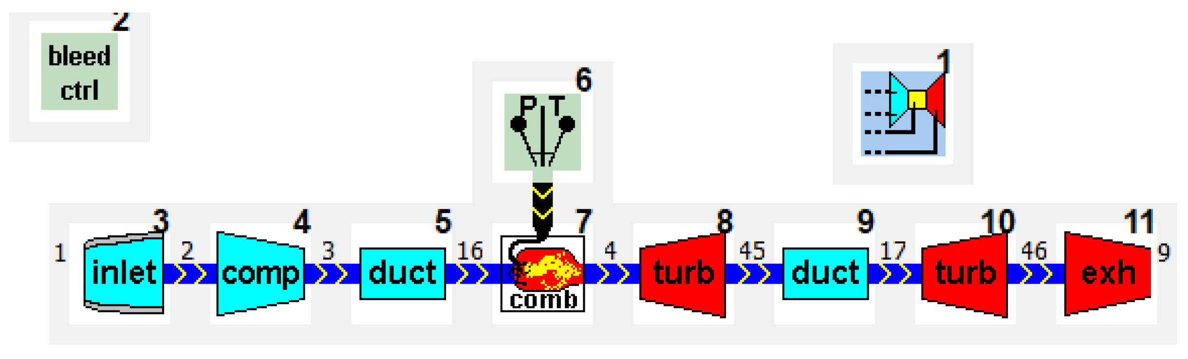
Figure 2.
PLA signal.
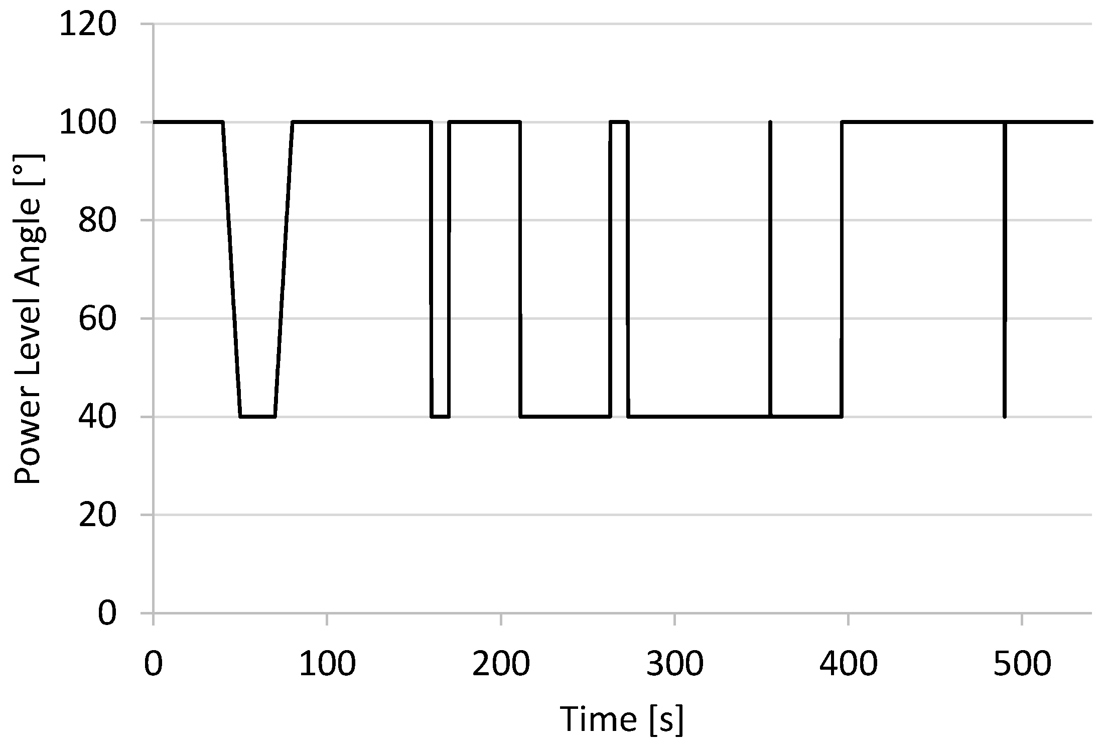
Figure 3.
Example of a feed-forward Artificial Neural Network.
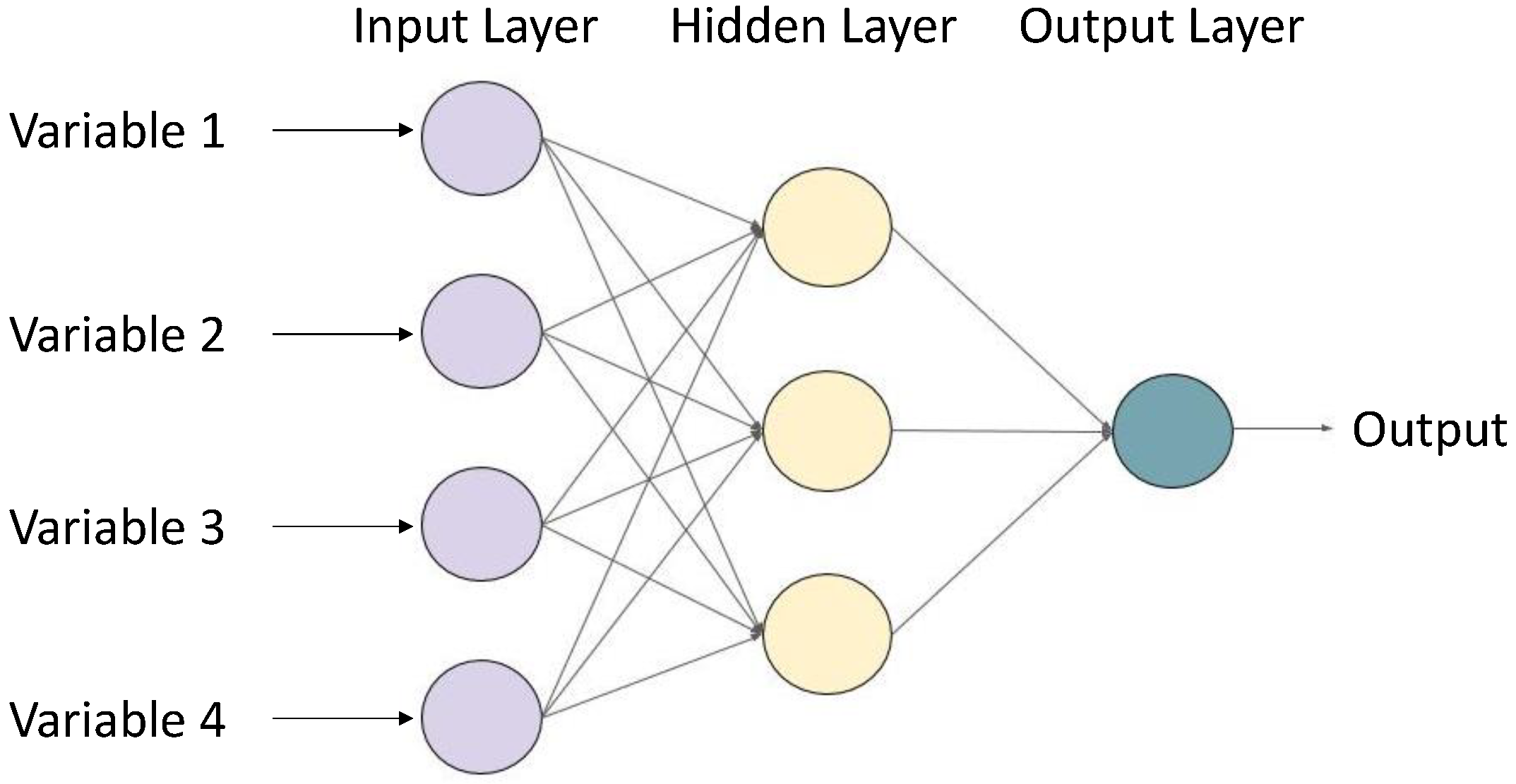
Figure 4.
Schematic diagram of a neuron.
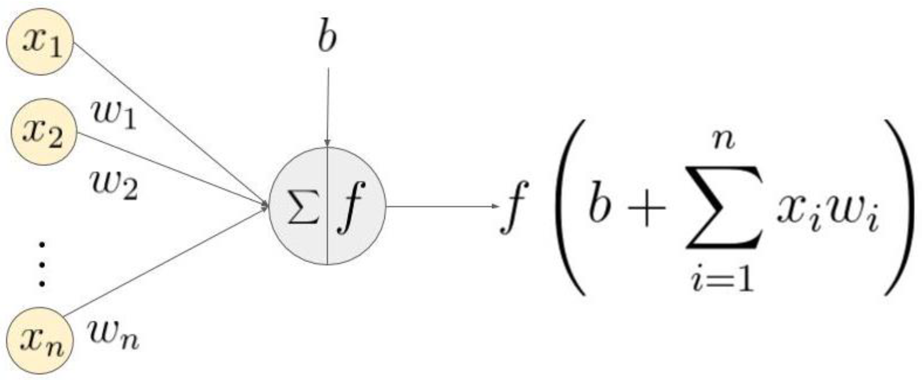
Figure 5.
NARX neural network.
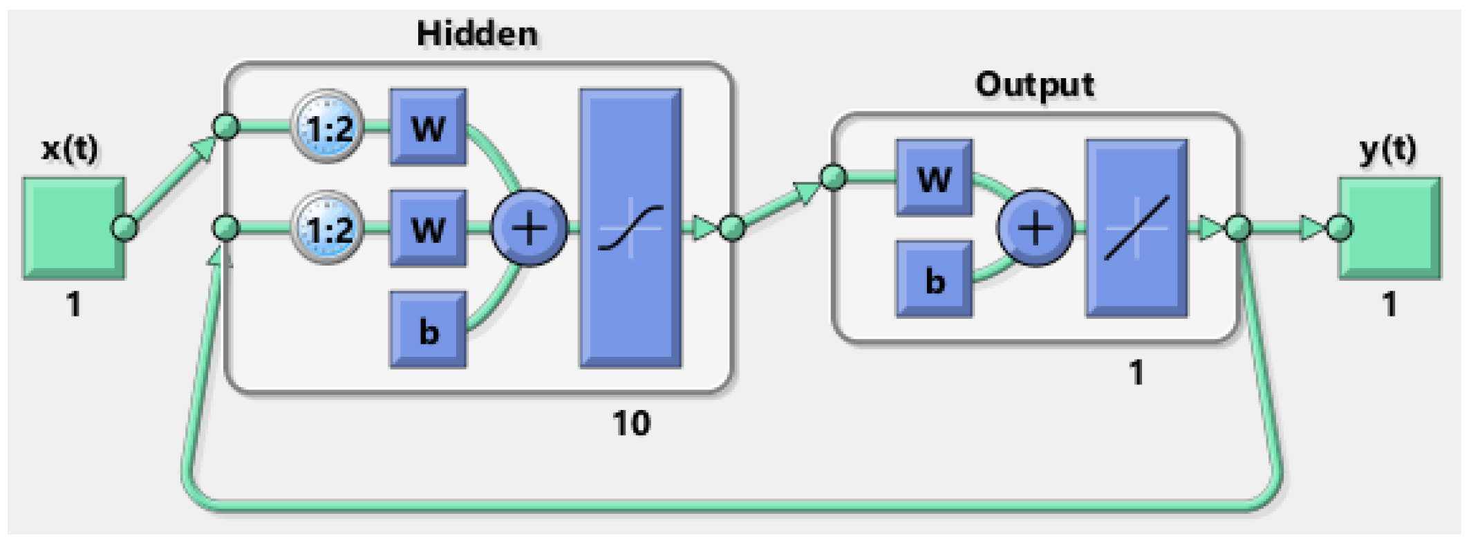
Figure 6.
Diagram of the complete NARX model: (a) first neural network; (b) second neural network.
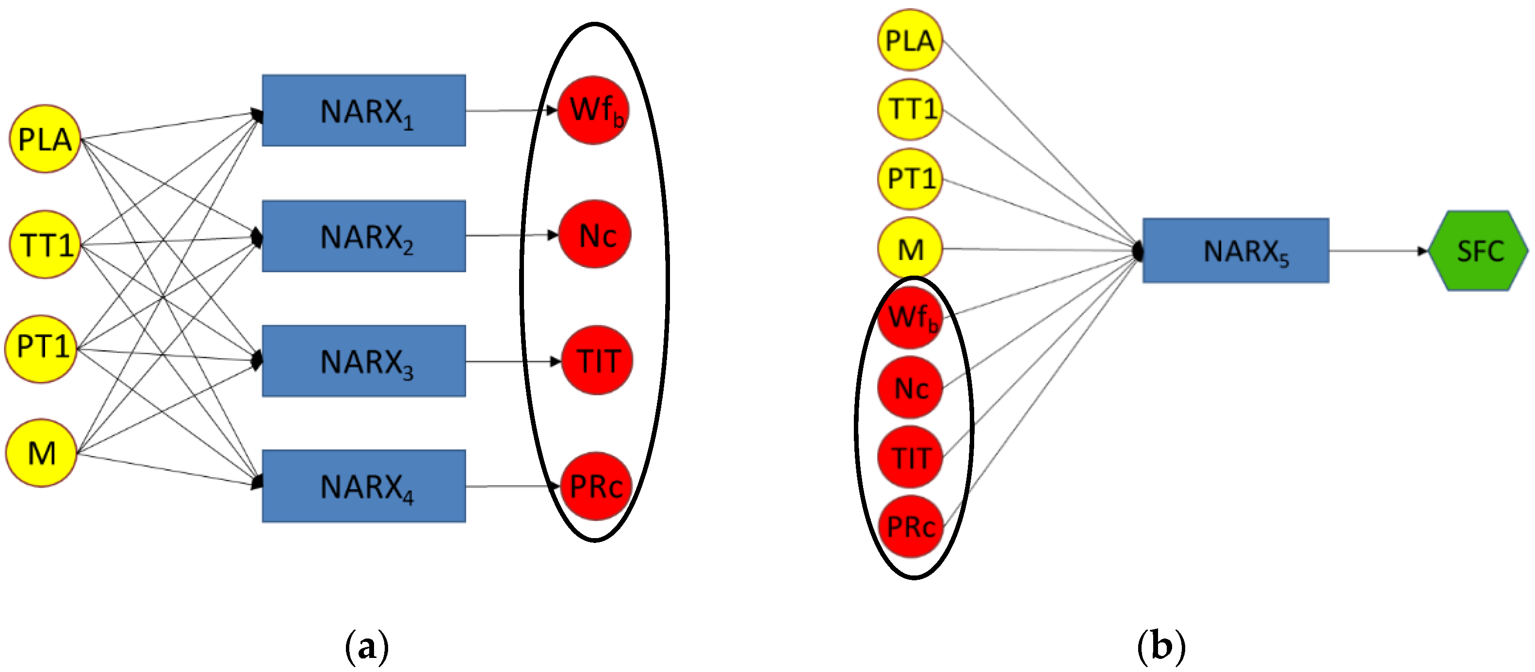
Figure 7.
Training (a) and testing (b) datasets.

Figure 8.
Loss Training curve for SFC parameter.

Figure 9.
RMSE (a) and R2 (b) of the NARX models for the training and test maneuvers for datasets in Figure 7.
Figure 9.
RMSE (a) and R2 (b) of the NARX models for the training and test maneuvers for datasets in Figure 7.

Figure 10.
Training (a) and testing (b) comparison between GSP and Net prediction of then ARX for the prediction of Wf_b under clean conditions (NARX1 Clean).
Figure 10.
Training (a) and testing (b) comparison between GSP and Net prediction of then ARX for the prediction of Wf_b under clean conditions (NARX1 Clean).
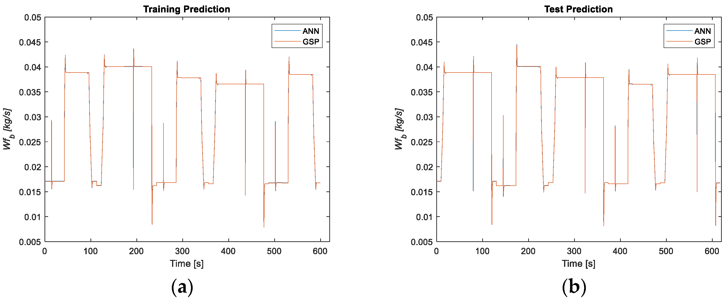
Figure 11.
Training (a) and testing (b) error comparison between GSP and Net prediction of the NARX for the prediction of Wf_b under clean conditions (NARX1 Clean).
Figure 11.
Training (a) and testing (b) error comparison between GSP and Net prediction of the NARX for the prediction of Wf_b under clean conditions (NARX1 Clean).
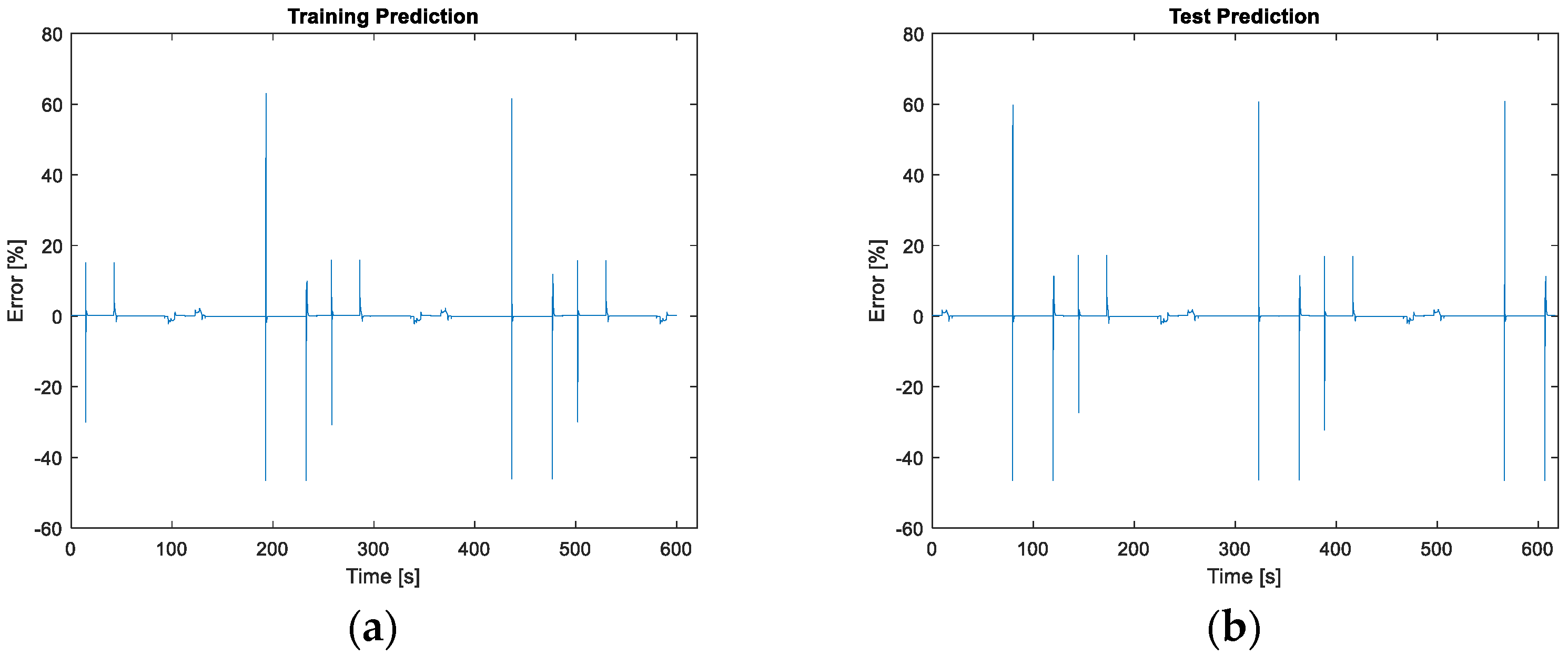
Figure 12.
Training (a) and testing (b) comparison between GSP and Net prediction of the NARX for the prediction of Nc under clean conditions (NARX2 Clean).
Figure 12.
Training (a) and testing (b) comparison between GSP and Net prediction of the NARX for the prediction of Nc under clean conditions (NARX2 Clean).

Figure 13.
Training (a) and testing (b) error comparison between GSP and Net prediction of the NARX for the prediction of Nc under clean conditions (NARX2 Clean).
Figure 13.
Training (a) and testing (b) error comparison between GSP and Net prediction of the NARX for the prediction of Nc under clean conditions (NARX2 Clean).
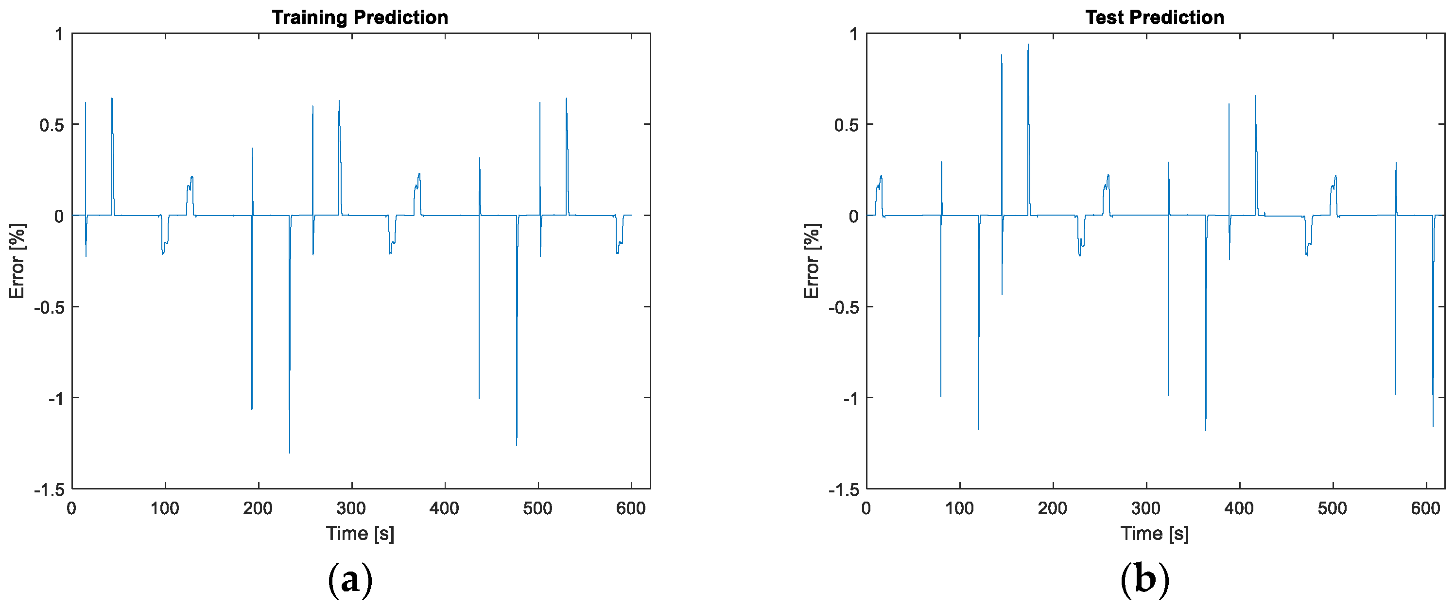
Figure 14.
Training (a) and testing (b) comparison between GSP and Net prediction of the NARX for the prediction of PRc under clean conditions (NARX3 Clean).
Figure 14.
Training (a) and testing (b) comparison between GSP and Net prediction of the NARX for the prediction of PRc under clean conditions (NARX3 Clean).
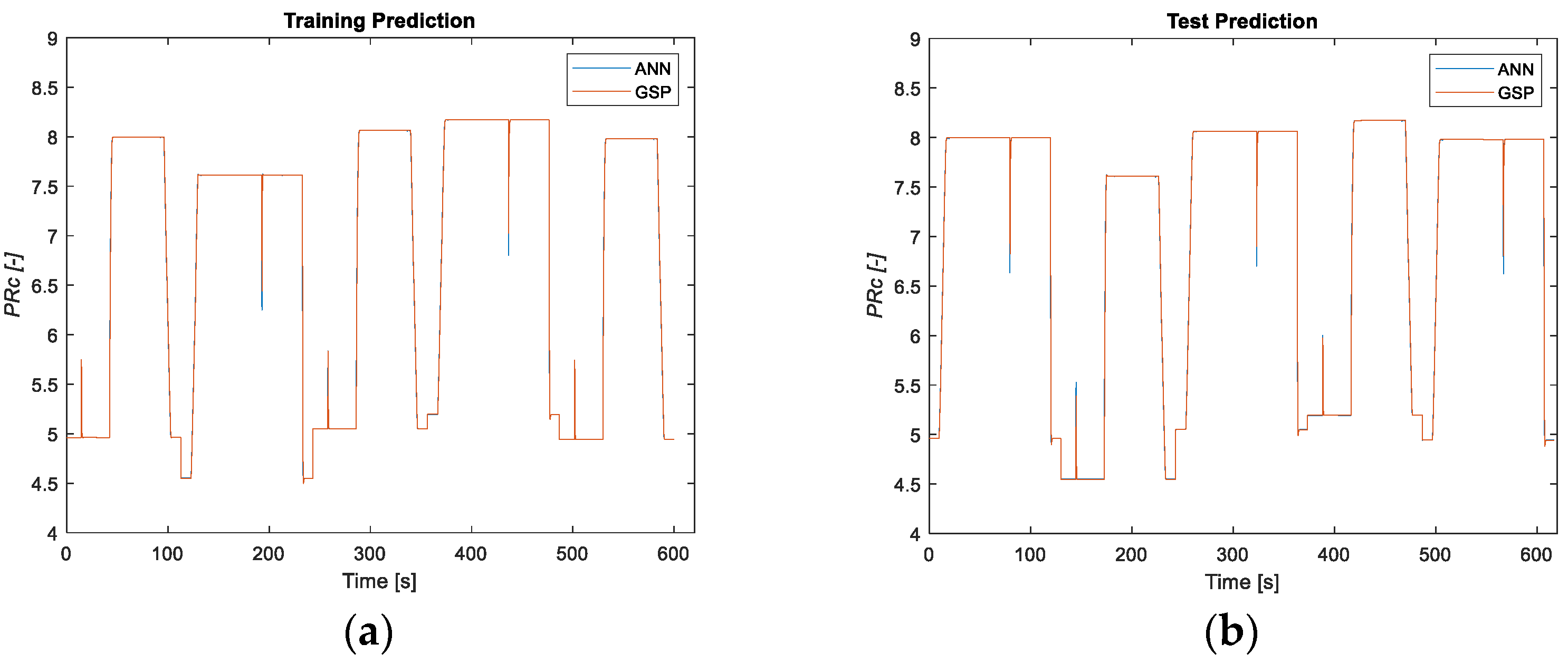
Figure 15.
Training (a) and testing (b) error comparison between GSP and Net prediction of the NARX for the prediction of PRc under clean conditions (NARX3 Clean).
Figure 15.
Training (a) and testing (b) error comparison between GSP and Net prediction of the NARX for the prediction of PRc under clean conditions (NARX3 Clean).
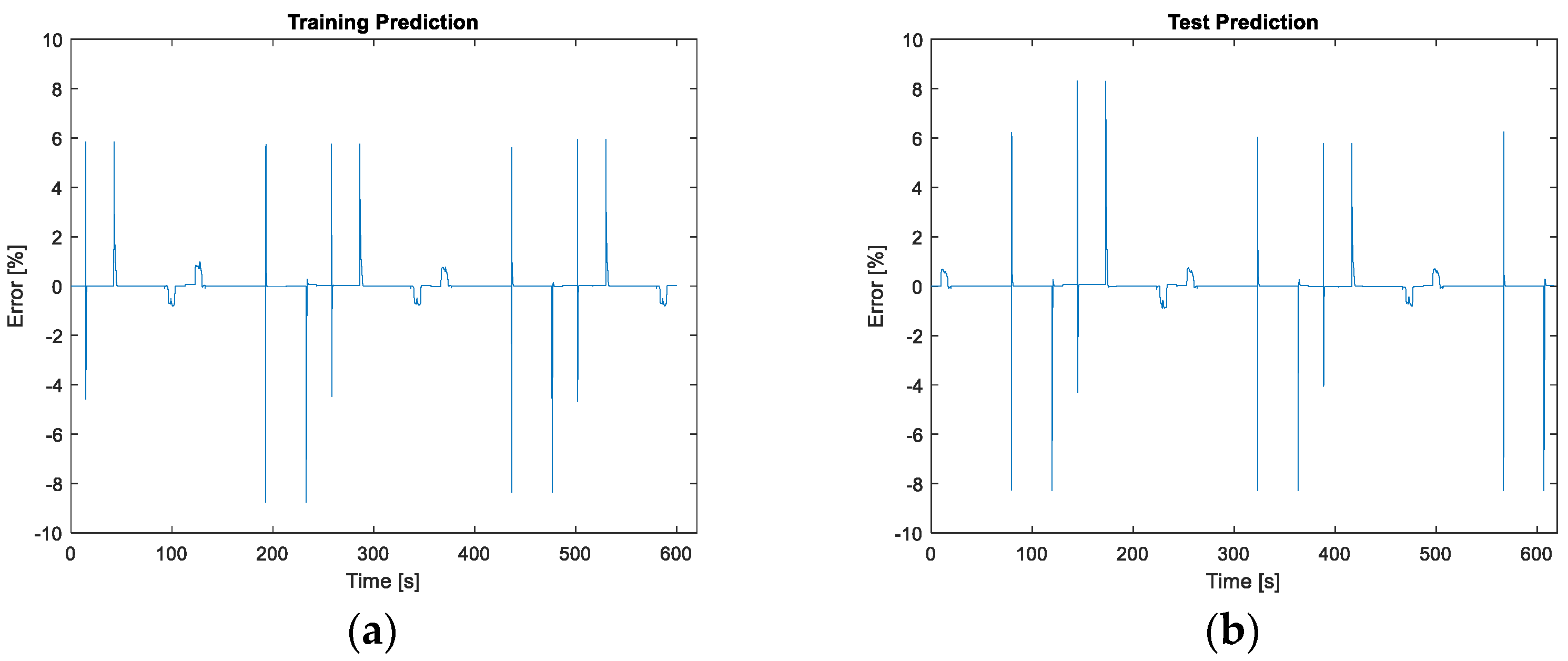
Figure 16.
Training (a) and testing (b) comparison between GSP and Net prediction of the NARX for the prediction of TIT under clean conditions (NARX4 Clean).
Figure 16.
Training (a) and testing (b) comparison between GSP and Net prediction of the NARX for the prediction of TIT under clean conditions (NARX4 Clean).

Figure 17.
Training (a) and testing (b) error comparison between GSP and Net prediction of the NARX for the prediction of TIT under clean conditions (NARX4 Clean).
Figure 17.
Training (a) and testing (b) error comparison between GSP and Net prediction of the NARX for the prediction of TIT under clean conditions (NARX4 Clean).

Figure 18.
Training (a) and testing (b) comparison between GSP and Net prediction of the NARX for the prediction of SFC under clean conditions (NARX5 Clean).
Figure 18.
Training (a) and testing (b) comparison between GSP and Net prediction of the NARX for the prediction of SFC under clean conditions (NARX5 Clean).
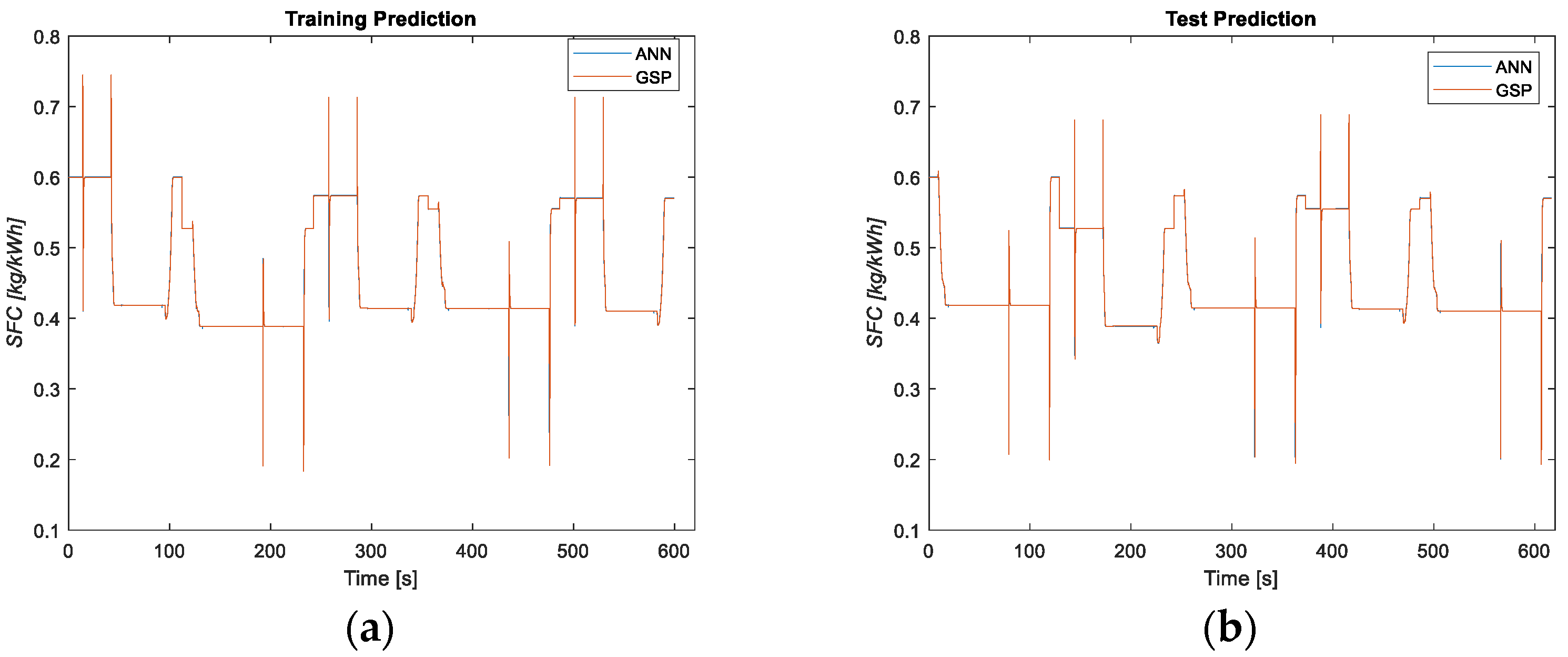
Figure 19.
Training (a) and testing (b) error comparison between GSP and Net prediction of the NARX for the prediction of SFC under clean conditions (NARX5 Clean).
Figure 19.
Training (a) and testing (b) error comparison between GSP and Net prediction of the NARX for the prediction of SFC under clean conditions (NARX5 Clean).
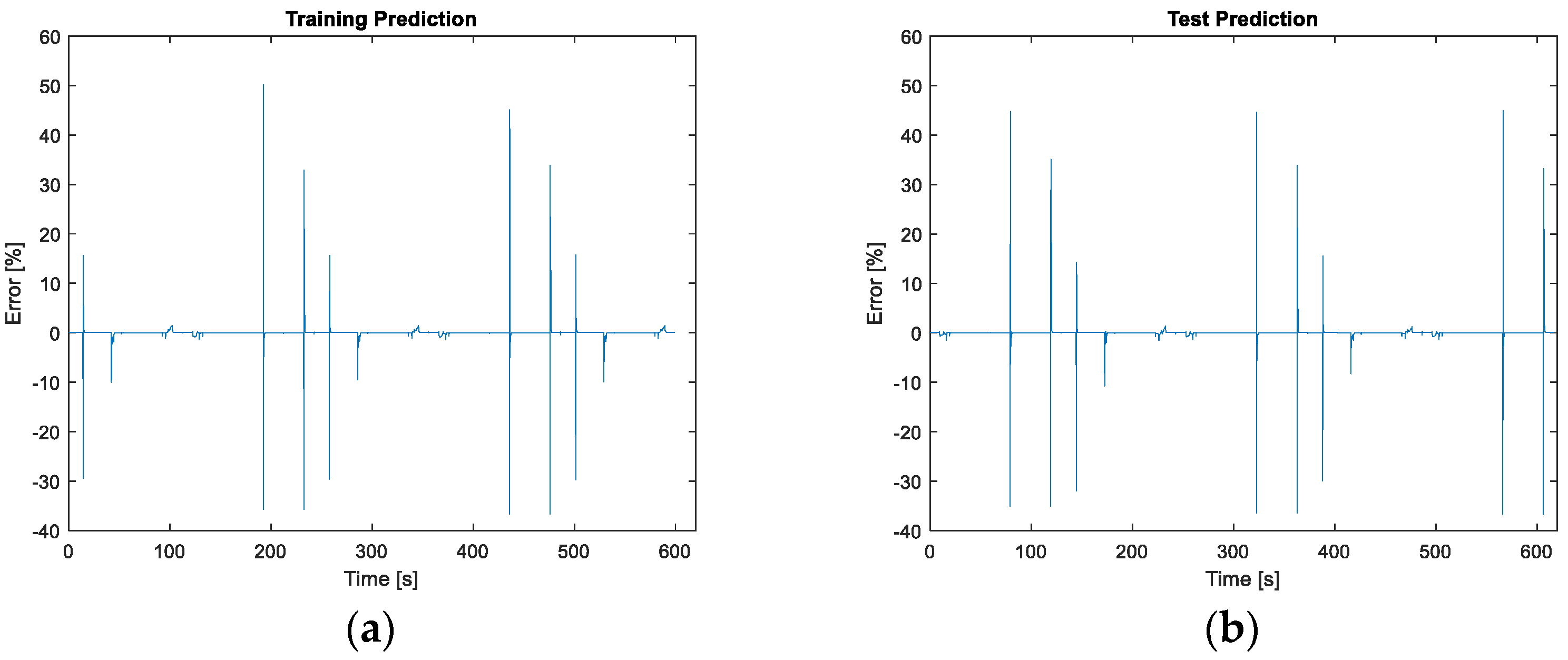
Figure 20.
Enlargement on the prediction of the SFC in steady-state conditions (PLA input “not aggressive”).
Figure 20.
Enlargement on the prediction of the SFC in steady-state conditions (PLA input “not aggressive”).
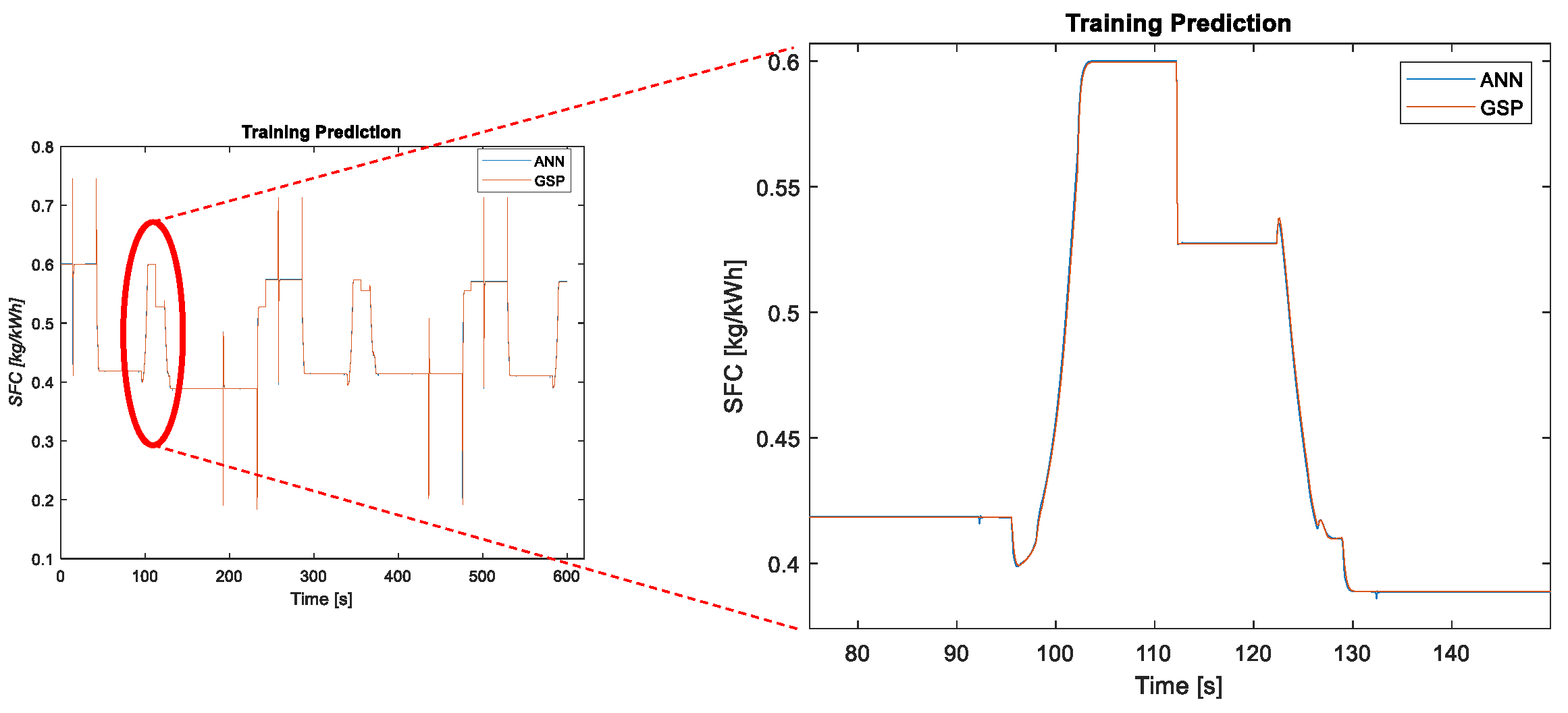
Figure 21.
SFC comparison between GSP and Net prediction under degraded conditions without adapting the ANN (NARX5 Clean) (a) and error in the SFC predictions (b).
Figure 21.
SFC comparison between GSP and Net prediction under degraded conditions without adapting the ANN (NARX5 Clean) (a) and error in the SFC predictions (b).
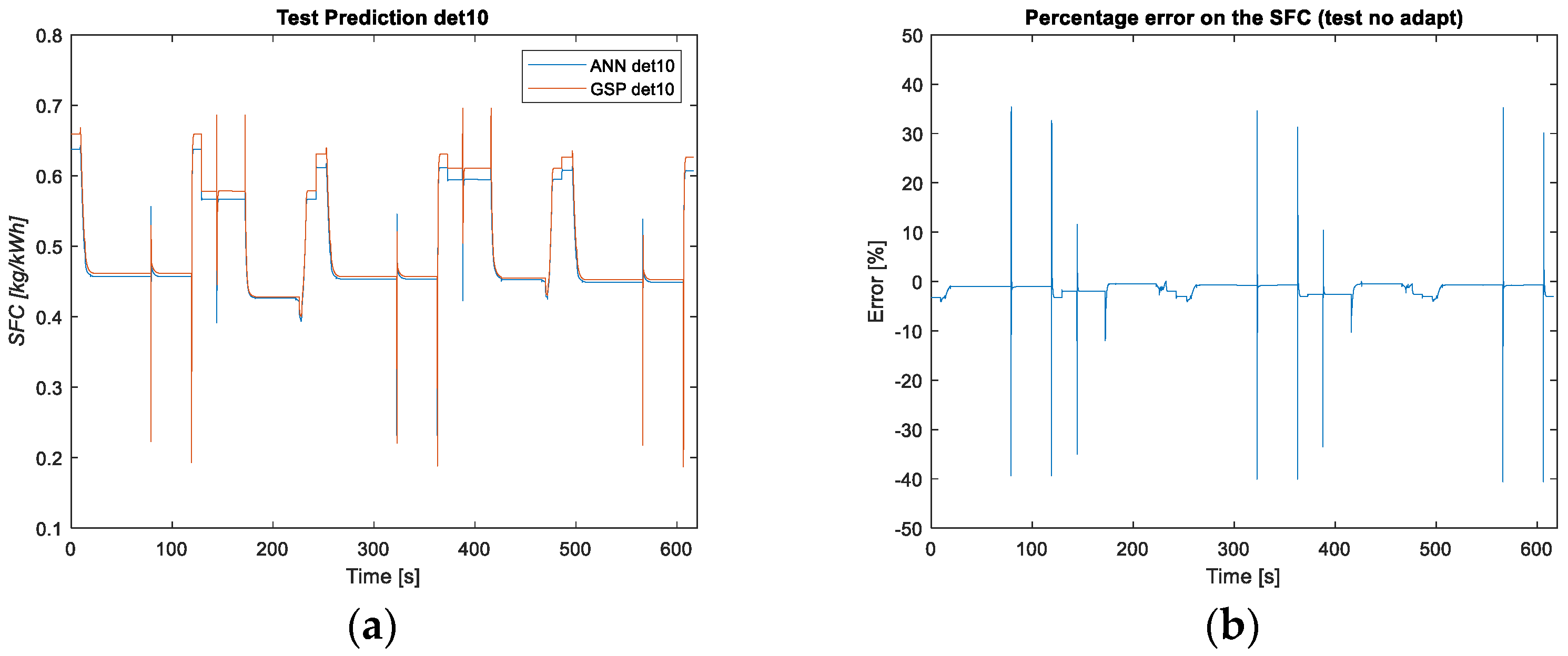
Figure 22.
Training (a) and testing (b) adapted SFC comparison between GSP and Net prediction under degraded conditions with adapting (NARX 5 Adapted).
Figure 22.
Training (a) and testing (b) adapted SFC comparison between GSP and Net prediction under degraded conditions with adapting (NARX 5 Adapted).
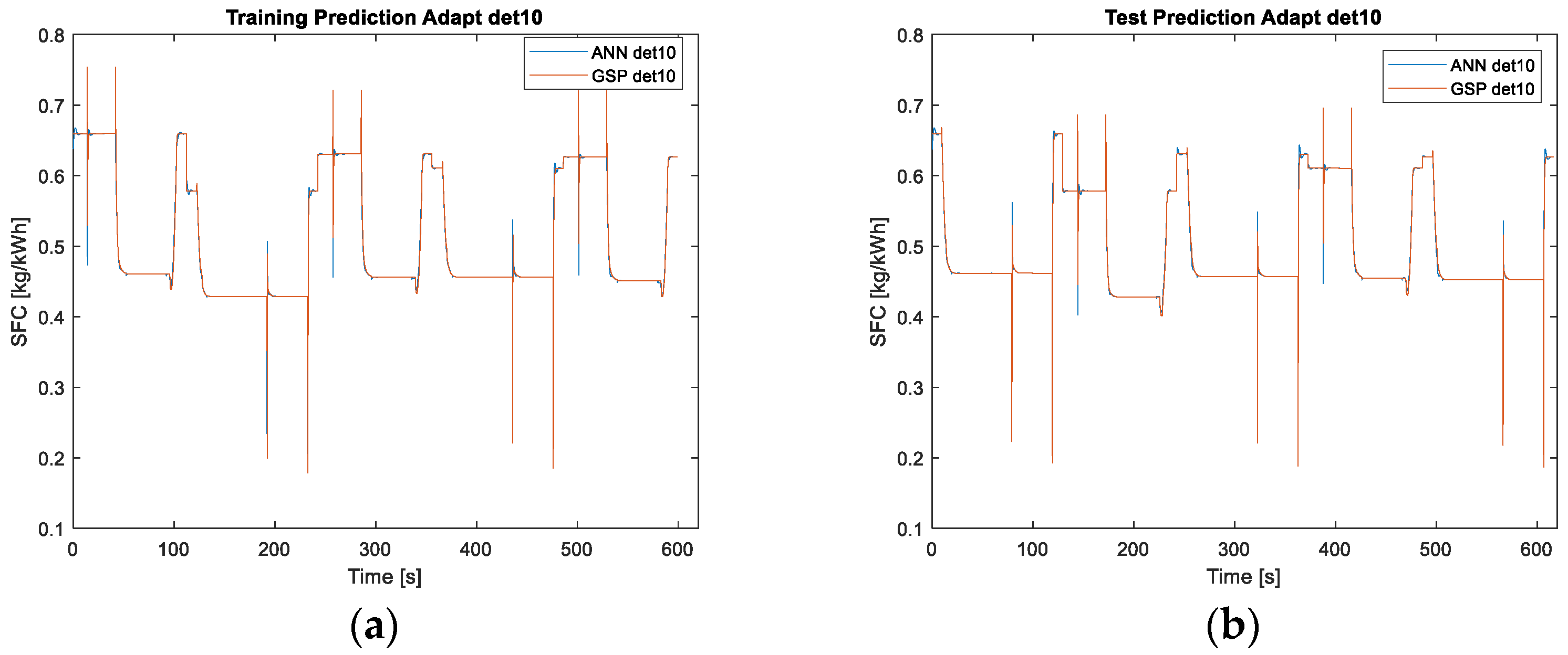
Figure 23.
Training (a) and testing (b) adapted SFC error comparison between GSP and Net prediction under degraded conditions with adapting (NARX 5 Adapted).
Figure 23.
Training (a) and testing (b) adapted SFC error comparison between GSP and Net prediction under degraded conditions with adapting (NARX 5 Adapted).
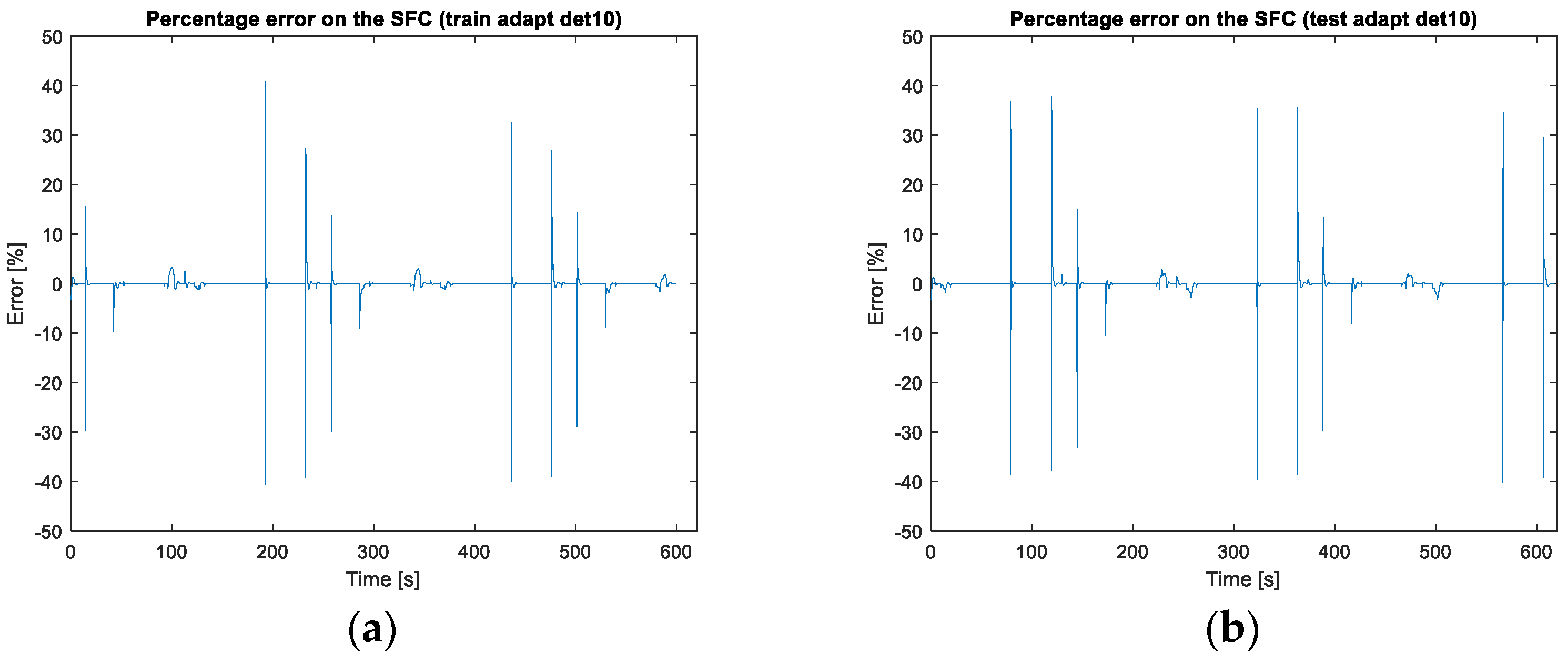
Figure 24.
Adjustment weights and biases in order to reach the target.

Table 1.
Specifications and configuration for the PW200.
| Description | Value |
|---|---|
| Power | 200–400 (kW) |
| Weight | 110 (kg) |
| Pressure Ratio | 8:1 |
| Turbine Inlet Temp | 1173.15 (K) |
| SFC (Specific Fuel Consumption) | 0.426–0.33 (kg/kWh) |
| Compressor Configuration | 1 centrifugal |
| Turbine Configuration (one stage) | HPT, LPT |
Table 2.
Design parameters for the PW200.
| Description | Value | Unit |
|---|---|---|
| Power (POW) | 266 | (kW) |
| Intake Pressure ratio (PR) | 0.988 | (-) |
| Air Flow rate (Wa) | 2 | (kg/s) |
| Combustion efficiency (ηb) | 0.985 | (-) |
| Fuel Flow rate (Wfb) | 0.0315 | (kg/s) |
| Compressor Rotor Speed (n1) | 40,891 | (rpm) |
| Compressor Efficiency (ηc) | 0.825 | (-) |
| LPT Rotor Speed (n2) | 6000 | (rpm) |
| Turbine efficiency (ηt) | 0.88 | (-) |
| Spool Mechanical Efficiency (ηm) | 0.99 | (-) |
Table 3.
Flight conditions.
| h [m] | Mach Number | |
|---|---|---|
| TO (Take-Off) | 0 | 0 |
| CR1 (Cruise1) | 313.5 | 0.45 |
| CR2 (Cruise2) | 400 | 0.12 |
| CR3 (Cruise3) | 800 | 0.09 |
| CR4 (Cruise4) | 313.5 | 0.21 |
Table 4.
Effects of various faults on component degradation.
| Physical Fault | Flow Capacity Change | Isentropic Efficiency Change |
|---|---|---|
| Compressor Fouling | ηc↓ | |
| Compressor Erosion | ηc↓ | |
| Compressor Corrosion | ηc↓ | |
| Compressor Blade Rubbing | ηc↓ | |
| Turbine Fouling | ηt↓ | |
| Turbine Erosion | ηt↓ | |
| Turbine Corrosion | ηt↓ | |
| Turbine Blade Rubbing | ηt↓ | |
| Thermal Distortion | ηt↓ | |
| FOD (Foreign Object Damage) | and | ηc↓ and ηt↓ |
Publisher’s Note: MDPI stays neutral with regard to jurisdictional claims in published maps and institutional affiliations. |
© 2021 by the authors. Licensee MDPI, Basel, Switzerland. This article is an open access article distributed under the terms and conditions of the Creative Commons Attribution (CC BY) license (https://creativecommons.org/licenses/by/4.0/).
Share and Cite
MDPI and ACS Style
De Giorgi, M.G.; Strafella, L.; Ficarella, A. Neural Nonlinear Autoregressive Model with Exogenous Input (NARX) for Turboshaft Aeroengine Fuel Control Unit Model. Aerospace 2021, 8, 206. https://doi.org/10.3390/aerospace8080206
AMA Style
De Giorgi MG, Strafella L, Ficarella A. Neural Nonlinear Autoregressive Model with Exogenous Input (NARX) for Turboshaft Aeroengine Fuel Control Unit Model. Aerospace. 2021; 8(8):206. https://doi.org/10.3390/aerospace8080206
Chicago/Turabian StyleDe Giorgi, Maria Grazia, Luciano Strafella, and Antonio Ficarella. 2021. "Neural Nonlinear Autoregressive Model with Exogenous Input (NARX) for Turboshaft Aeroengine Fuel Control Unit Model" Aerospace 8, no. 8: 206. https://doi.org/10.3390/aerospace8080206
Note that from the first issue of 2016, this journal uses article numbers instead of page numbers. See further details here.