Decentralized Control of Nanosatellite Tetrahedral Formation Flying Using Aerodynamic Forces

Abstract

A decentralized control algorithm for the construction of a tetrahedral configuration using differential lift and drag forces is proposed in this paper. Four 3U CubeSats launched in LEO are considered. Satellite attitude-controlled motion relative to the incoming airflow provides the required differential forces in order to change the relative translational motion. The developed control algorithm allows one to track the relative reference trajectories for the satellites at the vertices of the tetrahedron of the required shape and size. The influence of the initial launch conditions on the controlled tetrahedral motion is studied in this paper.

1. Introduction

One of the most important features of satellite formation flying is the ability to instantly measure the spatial distribution of parameters of interest in near-Earth space. Formation flying missions are used to study gravitational waves [1], Earth magnetosphere parameters [2,3], the stereo imaging of Earth surface [4], etc. In the case of 3D spatial scanning, at least four satellites are required. In an ideal case, the satellites should move at the vertices of the regular tetrahedron. Relative motion control must be applied to construct and maintain such a configuration. The control can be implemented using an onboard propulsion system [5,6] though for low-Earth orbits (LEOs), control can be implemented using differential aerodynamic forces [7,8].

The most famous tetrahedral satellite formation flying mission is the Magnetospheric Multiscale Mission for Earth magnetosphere studying [9]. Four satellites move along highly elliptical Earth orbits and are controlled using onboard thrusters via a ground command center. The implementation of such a mission using small satellites is restricted by their limited control abilities. The authors of [10] outlined the problem of designing and deploying a highly elliptical orbit tetrahedral formation of one controllable chief microsatellite and several passive deputy nanosatellites. A propellantless control approach using solar radiation pressure and atmospheric drag for reconfiguration maneuvers applied to a tetrahedral formation in highly elliptical orbits was proposed in [11]. Another idea is to use tethers to form the required tetrahedral formation. In [12], stationary configurations for a tethered tetrahedron were studied. It was shown in [13] that for low Earth orbits, it is possible to define such initial conditions of passive satellite motion that allow for the tetrahedron to preserve its volume and shape in a linear model. This type of tetrahedron has been considered for geomagnetic measurement exchange and interpolation in [14]. However, atmospheric drag and $J_2$ perturbation result in a relative drift between satellites, and translational control is required. In this paper, differential aerodynamic forces were applied to the problem.

Differential, drag-based, formation flying control is well-studied in the literature. Leonard first proposed such a control using the change of the satellites cross section area relative to the incoming airflow in 1986 [15]. Since then, a variety of algorithms based on this idea have been developed [8,16,17,18,19]. In 2013, Horsley et al. [20] proposed an idea to use the lift and drag components of aerodynamic force for formation flying control that also allowed them to control the relative out-of-plane and in-plane motion. A set of papers developed this idea and demonstrated control performance under J2 perturbations and atmospheric density uncertainties [21,22]. All the above-mentioned papers about differential forces control considered formations consisting of two satellites, and a centralized control approach was implemented. It is not clear how to use differential forces to achieve the required relative trajectories when there are more than two satellites. Decentralized control strategies or rules for implementation can be proposed for the task. In [23,24], cyclic and optimal control were proposed for a cluster flight. Another idea is to consider a communicational constraints, and decentralized control is based on neighbor satellite motion inside an individual communication sphere [25,26]. To the authors’ knowledge, the current paper is the first to propose decentralized control for differential lift and drag applications.

A set of papers were devoted to the problem of reference trajectory tracking control. A linear–quadratic regulator (LQR) is a widely implemented relative motion control algorithm for formation flying, and it was tested onboard the PRISMA [27] and CanX-4&5 [28] missions. In [29], a novel adaptive trajectory tracking algorithm for a space manipulator was proposed; it guarantees a prescribed performance while considering actuator saturation. An adaptive guidance architecture using Guardian Map was developed in [30]; it provides asymptotic convergence to the fuel-efficient natural trajectories of formation flying in elliptical orbits. The neural-network-based adaptive controller from [31] is able to tune algorithm parameters for better trajectory tracking in cases of uncertainties in dynamical disturbances acting on deep-space formation flying. In our work, LQR-based control was applied to the tracking of an average deviation from three relative trajectories at the same time for tetrahedral formation flying.

The purpose of this paper was to develop and study a decentralized algorithm for group satellite control after launch to construct a tetrahedral configuration. 3U CubeSats motion after deployment from the launcher is considered. An LQR-based decentralized control algorithm to track the relative reference trajectory is proposed. The reference trajectory of the satellites was selected to obtain a tetrahedron of required quality. The convergence time, depending on the initial conditions and tetrahedron size, is investigated.

2. Problem Statement

The problem of satellite tetrahedral formation construction after launch is considered because it is necessary to achieve defined relative trajectories in order to provide satellite motion in the vertices of a tetrahedron of required size. Each satellite is given information about the relative motion of other satellites. This information is obtained via an inter-satellite link or using an autonomous relative motion determination system.

Consider a formation launched in LEO: each satellite is assumed to be equipped with an attitude control system. Thus, the satellites’ relative motion can be controlled by the difference in aerodynamic forces, which depends on the attitude of the satellites relative to the incoming airflow. The 3U CubeSats considered in this paper have a form-factor that is suitable for differential aerodynamic control. The goal of the work was to develop decentralized aerodynamic control to construct the tetrahedral formation.

2.1. Motion Equations

The Hill–Clohessy–Wiltshire relative motion equations [32,33] for two satellites in near circular orbits in a central gravitational field were considered for control algorithm development. These equations were written in the orbital reference frame, the origin of which moves along the circular orbit with radius $r_0$. The $Oz$ axis is aligned along the nadir direction, the $Oy$ axis is directed along the orbital momentum vector, and the $Ox$ axis complements the triad (Figure 1).

Consider two 3U CubeSats with the radius-vectors $r_i=(x_i,y_i,z_i)$ and $r_j=(x_j,y_j,z_j)$ for i-th and j-th satellites written in the orbital reference frame. The relative radius-vector $r_{ij}=r_j-r_i=(x_{ij},y_{ij},z_{ij})$ components change according to the following equations:

$$\{\begin{array}{l}{\ddot{x}}_{ij}+2\omega {\dot{z}}_{ij}=u_x^{ij},\\ {\ddot{y}}_{ij}+{\omega }^2{y}_{ij}=u_y^{ij},\\ {\ddot{z}}_{ij}-2\omega {\dot{x}}_{ij}-3{\omega }^2{z}_{ij}=u_z^{ij},\end{array}$$

(1)

where $\omega =\sqrt{\mu /r_0^3}$ is the orbital angular velocity, $\mu$ is the Earth gravitational parameter, $u_{ij}=\Delta f_{ij}/m,$ $\Delta f_{ij}=f_j-f_i$ is the difference between the aerodynamic forces acting on the i-th and the j-th satellites, and $m$ is the mass of the satellites. For the case of free motion, the solution of Equation (1) is as follows

$$\{\begin{array}{l}{x}_{ij}(t)=-3C_1^{ij}\omega t+2C_2^{ij}\cos (\omega t)-2C_3^{ij}\sin (\omega t)+C_4^{ij},\\ y_{ij}(t)=C_5^{ij}\sin (\omega t)+C_6^{ij}\cos (\omega t),\\ z_{ij}(t)=2C_1^{ij}+C_2^{ij}\sin (\omega t)+C_3^{ij}\cos (\omega t),\end{array}$$

where $C_1^{ij}-C_6^{ij}$ are trajectory parameters dependent on the initial conditions at $t=0$.

2.2. Aerodynamic Force Model

Assume that the i-th and j-th satellites are the identical 3U CubeSats and their shape is rectangular parallelepiped with a size of 10 × 10 × 30 cm. The satellites are equipped with solar panels that cover the bodies of the satellites. For simplicity, consider that the satellites rotate in a way that only one of the greater sides of each satellite (30 × 10 cm²) is affected by the incoming airflow. The other two greater sides are always perpendicular to the velocity vector, and the last one is in the shadow relative to the incident flow. Only one of the two smaller sides (10 × 10 cm²) can be directed toward the velocity vector of the satellites.

Consider an aerodynamic force model that accounts the lift component [34]. The outer unit normal vector $n_k$ to the $k$-th side of the CubeSat can be written as follows:

$$n_k=\left[\begin{array}{c}\sin {\theta }_k\\ \cos {\theta }_k\cos {\phi }_k\\ \cos {\theta }_k\sin {\phi }_k\end{array}\right].$$

where the angle ${\theta }_k$ is chosen such that the aerodynamic force does not act on the satellite when ${\theta }_k=0$. ${\theta }_k\in [0;\pi /2]$; if ${\theta }_k<0$, then the other side of the CubeSat should be considered. Additionally, angle ${\phi }_k\in [0,2\pi )$. Assume that the vector of the incoming airflow is directed along the $Ox$ axis, as this is an adequate assumption for near circular orbits. In this case, the aerodynamic force has the following expression in the orbital reference frame [22]:

$$f_k=K\left[\begin{array}{c}-2\epsilon {(\sin {\theta }_k)}^3+\eta (\epsilon -1){(\sin {\theta }_k)}^2+\left(\epsilon -1\right)\sin {\theta }_k\\ -\cos {\theta }_k\sin {\theta }_k(\eta -\epsilon \eta +2\epsilon \sin {\theta }_k)\cos {\phi }_k\\ -\cos {\theta }_k\sin {\theta }_k(\eta -\epsilon \eta +2\epsilon \sin {\theta }_k)\sin {\phi }_k\end{array}\right],$$

(2)

where $K=\frac{1}{m}\rho V^2{S}_k$, $\rho$ is the atmosphere density, $V$ is the airflow velocity, $S_k$ is the CubeSat side area, and $\epsilon$ and $\eta$ are constant parameters describing the interaction of molecules with the surface. To calculate the overall aerodynamic force acting on the $i$-th satellite, all the forces with ${\theta }_k>0$ for the outer normal vector to the satellite sides should be summarized:

$$f_i={\displaystyle \sum _{k=1}^6{f}_k},\mathrm{if}{\theta }_k\ge 0.$$

The resulting control force is the difference between the forces acting on two satellites:

$$\Delta f_{ij}=f_j-f_i$$

(3)

In case of two satellites in formation, the control force is the function of the attitude angles, which is defined as ${\theta }_k,{\phi }_k$ for each side of each CubeSat. However, if there are four satellites in the group, there are three reference relative trajectories for each satellite and a control strategy should be defined.

3. Control Algorithm

Consider an application of the linear quadratic regulator to track the predefined relative trajectory. This control algorithm is quite simple to implement in the case of two satellites in a group, but an additional decentralized control rule is needed in the case of N satellites. In this section, an LQR is constructed and the decentralized approach is proposed.

3.1. LQR Basics

An LQR can be applied for linear systems with the following relative motion equations:

$${\dot{x}}_{ij}=A{x}_{ij}+B{u}_{ij}$$

(4)

where the state vector $x_{ij}$ for our case consists of radius-vector and velocity in the orbital reference frame, $x_{ij}={[r_{ij}^T{v}_{ij}^T]}^T$ is the state vector, $A$ is the dynamic matrix,

$$A=\left[\begin{array}{cc}{0}_{3\mathrm{x}3}& E\\ C& D\end{array}\right],$$

$E$ is the identity matrix with a size of 3 × 3,

$$C=\left[\begin{array}{ccc}0& 0& 0\\ 0& -{\omega }^2& 0\\ 0& 0& 3{\omega }^2\end{array}\right],D=\left[\begin{array}{ccc}0& 0& -2\omega \\ 0& 0& 0\\ 2\omega & 0& 0\end{array}\right],$$

and $B$ is the control matrix

$$B=\left[\begin{array}{c}{0}_{3\mathrm{x}3}\\ E\end{array}\right].$$

The reference trajectory can be obtained through the integration of the free motion equations:

$${\dot{x}}_{ij}^d=A{x}_{ij}^d$$

where $x_{ij}^d$ is the reference trajectory state vector. For the deviation from the reference trajectory $e=x_{ij}-x_{ij}^d$, the equation has the following form:

$${\dot{e}}_{ij}=A{e}_{ij}+B{u}_{ij}$$

(5)

The LQR is the feedback control of the form $u=-K_{c}e$ that minimizes the following functional [35].

$$J={\displaystyle \underset{0}{\overset{\infty }{\int }}(e_{ij}^{T}Q{e}_{ij}+u_{ij}^{T}R{u}_{ij})dt}$$

(6)

where $K_c$ is the control gain matrix and matrices $Q,R$ are the positive definites that determine the weight of errors for the state vector and the weight of the control resource consumption, respectively. The control vector is defined by the equation

$$u_{ij}=-R^{-1}{B}^{T}P{e}_{ij}$$

(7)

where the matrix $P$ is obtained from the solution of the Riccati equation

$$A^{T}P+PA-PB{R}^{-1}{B}^{T}P+Q=0.$$

(8)

3.2. Average Deviation from the Reference Trajectories

The main challenge of the LQR application to tetrahedral formation control is that for each satellite, there are three reference trajectories relative to each of the rest of the satellites. The reference relative trajectories are chosen in a way that during motion, all the four satellites are located in the vertices of the tetrahedron of required size. Thus, control from Equation (7) should be applied according to each trajectory deviation. However, the deviations $e_{ij}$ could lead to completely different control vectors $u_{ij}$. That is why a decentralized control strategy has to be defined for the construction of a tetrahedral formation. One way to solve this problem is to use an average deviation. The mean vector of the deviations ${\overline{e}}_i$ for each satellite is as follows:

$${\overline{e}}_i={\displaystyle \sum _{j=1}^3{e}_{ij}}/3.$$

The resulting control vector can be calculated using Equation (7):

$${\overline{u}}_i=-R^{-1}{B}^{T}P{\overline{e}}_i$$

(9)

Thus, the proposed control leads to the convergence of the mean trajectory deviation to zero; the relative trajectories reach the reference trajectories, and the required tetrahedron motion is obtained.

3.3. Constraints of the Differential Aerodynamic Forces

The decentralized control approach means that each satellite is individually and independently controlled based on the relative motion of the neighbor satellites. The differential force is the difference between each pair of the satellites, which means that the i-th satellite can partly implement the calculated control. According to the aerodynamic force model, the force component in the along-track direction is always negative, and the possible values are inside the interval $u_i^x\in [-u_{\max }^x;-u_{\min }^x]$, where $u_{\max }^i>0$ represents the maximum and minimum values that correspond to CubeSat positions of maximum and minimum cross-section area relative to the incoming airflow.

Thus, it is assumed that in the case of the control saturation, it is necessary to implement maximum possible components along the Ox axes, but according to the force model in this case, the other components are zero: $u_{\max }^x=\left[-u_{\max }^{x}00\right]$. In the case that the calculated control ${\overline{u}}_i$ is in the acceptable control region, it can be implemented. However, in the case that the calculated average deviation control ${\overline{u}}_i^x$ is of a negative value, then its vector $u_i$ cannot be implemented and set to a minimum value corresponding to $u_{\min }^x=\left[-u_{\min }^{x}00\right]$. When $0<{\overline{u}}_i^x<u_{\max }^x$ in the acceptable control region but the sum of the other two components are saturated, i.e., $\sqrt{{\left({\overline{u}}_i^y\right)}^2+{\left({\overline{u}}_i^z\right)}^2}>u_{\max }^{yz}$, it is reasonable to implement its maximum value $u_{\max }^{yz}$. However if the angle $\theta \approx 52$ degrees for the largest side of the CubeSat and the Ox component ${\tilde{u}}_i^x$ at this angle is $u_i^x/K\approx 0.8$, the control vector to be applied in that case is $u_{\max }^{yz}=\left[{\tilde{u}}_i^x{\overline{u}}_i^y/u_{\max }^{yz}{\overline{u}}_i^z/u_{\max }^{yz}\right]$, i.e., the calculated values for the Oy and Oz values are normalized to the maximum possible value $u_{\max }^{yz}$.

In summation, for $u_i$, one can propose the following decentralized control law:

$$u_i=\{\begin{array}{l}-u_{\max }^x,\mathrm{if}{\overline{u}}_i^x>u_{\max }^x,\\ -u_{\max }^{yz},\mathrm{if}0<{\overline{u}}_i^x<u_{\max }^x,\\ \mathrm{and}\sqrt{{\left({\overline{u}}_i^y\right)}^2+{\left({\overline{u}}_i^z\right)}^2}>u_{\max }^{yz},\\ -{\overline{u}}_i,\mathrm{if}0<{\overline{u}}_i^x<u_{\max }^x,\\ -u_{\min }^x,\mathrm{if}{\overline{u}}_i^x<0.\end{array}$$

(10)

The proposed decentralized control strategy was empirically derived based on practical logic, and its values were partly based on the LQR because it considers aerodynamic force value constrains. Thus, algorithm performance needed to be demonstrated. Due to actual aerodynamic force restrictions, the convergence of the relative deviations of the trajectories cannot be analytically proved. That is why only numerical simulations were used for the controlled motion study.

4. Numerical Study

Consider the application of the proposed control algorithm for tetrahedron construction. The control is developed under assumptions of linear motion equations, a circular orbit, and a constant atmosphere density. In this section, we discuss the results of a numerical study using the simulation of orbital motion that considered the orbit eccentricity, the second harmonic $J_2$, and the GOST atmosphere model of upper Earth atmospheric density [36]. Thus, the performance of controlled motion in presence of disturbances and density uncertainty is analyzed.

The simulation start time was set as 1 January 2020, 0:00 a.m. For this date, all the parameters required for the atmosphere density model were used. The 3U CubeSat cluster launch scheme was considered. It was assumed that the satellites were separated from the launcher in the Ox axis direction one after another, with the time interval $\Delta t$ between the launches. The velocity of the ejection $V_e$ was assumed to be the same for all the CubeSats, but due to launch system inaccuracy, the ejection velocity was subjected to errors. Thus, the initial velocity vector $V_0$ in the orbital reference frame was modelled as follows:

$$V_0=\left[\begin{array}{c}{V}_e+\delta V\\ \delta V\\ \delta V\end{array}\right],$$

(11)

where $\delta V$ is the ejection error considered to be a normally distributed random value with zero mean and a covariance of ${\sigma }_{\delta V}^2$.

After separation, the implementation of control aimed at achieving the tetrahedral formation began. A tetrahedron with the best quality was accomplished if the satellites move along the following reference orbits [37]:

$$\begin{array}{l}{x}_1=2A\cos (\omega t-\arccos (1/3)),\\ y_1=A\sqrt{3}\sin (\omega t),\\ z_1=A\sin (\omega t-\arccos (1/3)),\\ \\ x_2=2A\cos (\omega t),\\ y_2=A\sqrt{3}\sin (\omega t+\arccos (1/3)),\\ z_2=A\sin (\omega t),\end{array}\begin{array}{l}{x}_3=D,\\ y_3=0,\\ z_3=0,\\ \\ x_4=-D,\\ y_4=0,\\ z_4=0,\end{array}$$

(12)

where $r_i={[x_i{y}_i{z}_i]}^T$ represents the radius-vector of i-th satellite in the orbital reference frame and $A\mathrm{and}D$ are constants. According to that equation, two of the satellites were moving along the same the circular path with a constant separation equal to 2D. The other two satellites were moving along the circular relative trajectories with the angular separation shown in Figure 2.

All the parameters used in the simulation of the controlled motion of the CubeSat formation flying are presented in

Table 1. Parameters and initial conditions of the numerical simulation.

Main Parameters of the Formation
Number of satellites in the formation	4
Time interval between control calculation, $\Delta T$	150 s
Orbit attitude, $h$	340 km
Orbit inclination, i	51.7 deg
Parameter of tetrahedron A	100 m
Parameter of tetrahedron D	115 m
Launch Parameters
Time interval between the launches, $\Delta t$	10 s
Ejection velocity, $V_e$	0.5 m/s
Ejection error deviation, ${\sigma }_{\delta V}^{}$	0.015 m/s
CubeSat Parameters
Mass of satellite, $m$	3 kg
Difference between maximum and minimum value of the cross-sectional area, $\Delta S$	0.02 m2
Aerodynamic drag coefficient, $C_a$	2
LQR Parameters
Matrix $Q$	$E_{6\mathrm{x}6}$
Matrix R	diag ([${10}^{-13};{10}^{-14};{10}^{-14}$])
Aerodynamic Force Parameters
Constant atmosphere density, $\rho$	${10}^{-11}$ kg/m3
Airflow velocity, $V=\sqrt{\mu /(R_E+h)}$	7.69 km/s
Parameters $\epsilon$ and $\eta$	0.1
Maximum of the control source, $u_{\max }$	$4.1\cdot {10}^{-6}$ m/s2

. The constant atmosphere density corresponding to the average density for altitude of 340 km was used for the control calculation, though the actual atmosphere density corresponded to the GOST model. Thus, the density uncertainty for the decentralized algorithm was simulated.

Figure 3 shows the relative trajectories of the three satellites relative to the forth satellite in the case of uncontrolled motion. One can see that the relative trajectories were diverging along the Ox axes due to initial launch velocity errors. Figure 4 demonstrates the relative motion trajectories under the proposed decentralized control Equation (10). One can see that the trajectories relative to the fourth satellite converged to the desired trajectory described by Equation (12).

Figure 5 presents the vector deviations relative to the fourth satellite. One can see that all the deviations after approximately 35 h finally converged to a zero vicinity of a few meters. The slowest convergence had the Oy component of the vector deviations due to relatively small lift component of the aerodynamic force. The final tracking error of the required tetrahedron was about 1 m, and it was caused by control implementation errors and $J_2$ perturbation.

The calculated control according to Equation (9) for the average relative vector deviations for all the satellites is presented in Figure 6, and the corresponding implemented value according to Equation (10) is shown in Figure 7. The control vectors were divided by the aerodynamic force coefficient $K$ from Equation (2) and are presented in dimensionless units for convenience. One can see that in the beginning of the simulation, the calculated control value for the Ox component was positive for some time intervals. This could not be realized by aerodynamic force, so its value was set to zero in the implemented control algorithm according to Equation (10). After approximately 3 h, the deviation along the Ox axis considerably decreased, but all the positive calculated values were still not implemented. After 3 h, the deviation along the Oy axis still was large enough to lead to saturation for the corresponding control vector component. During this case that lasted for approximately the next 20 h, the second control situation from Equation (10) was implemented. It caused a temporarily increased deviation along the Ox axis. However, after 23 h, the deviations along the Oy axis decreased and all of the components of the calculated control fell into the acceptable control region.

It is possible that the proposed decentralized control algorithm could fail to construct a tetrahedral configuration in a case of implemented control saturation for a long time period (several orbital periods). This could be the result of incorrectly chosen weight matrices Q and R in the LQR. In order to avoid the implemented control saturation, preliminary deviations from the required trajectories should be estimated using a priori information of the launch’s initial conditions. Then, the weight matrices Q and R should be selected in such a way that the calculated LQR-based control from Equation (9) is inside an acceptable control region that could be implemented by aerodynamic forces. The methodology for these parameter selections is described in [22]. Though the LQR parameters were correctly chosen in the presented simulation example, there was a temporary saturation of the implemented control. Despite the control implementation errors at the initial time of simulation, the proposed control the convergence to the required trajectories.

Figure 8 presents the change in orbit altitude of the satellites in formation flying. Over 60 h of simulation, the altitude decreased by about 300 m. At the beginning of the simulation, the required control in the along-track direction was significant, so it caused faster orbit degradation. In first 10 h, altitude decreased by more than 100 m. Afterwards, the cross-section relative to the incoming airflow was about the minimum value of 0.01 m². The orbit degradation continued but at a slower rate. Figure 9 presents the GOST model of atmosphere density, which considers the day–night variation and current solar activity. The control was calculated using a constant density model without actual density information. This led to certain implementation control errors that influenced the trajectory performance.

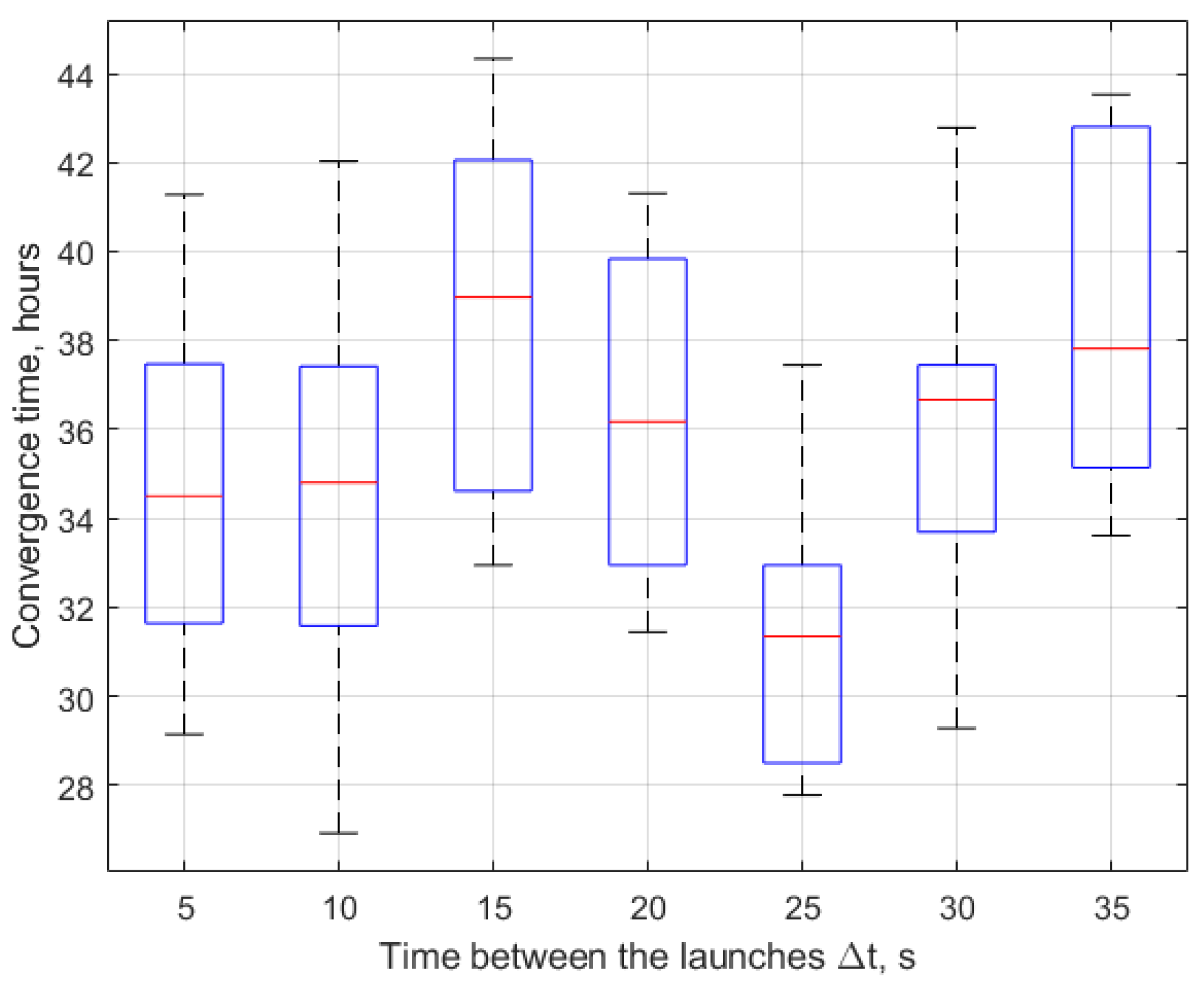
It was important to investigate the time that is needed to construct the tetrahedral flying formation depending on launch conditions. A set of the possible time intervals between the launches was considered, and the time of tetrahedral construction was numerically estimated. It was assumed that the configuration was formed if the deviations of all the trajectories from the reference trajectories were less than 5 m. Twenty simulations for each time interval were carried out. Since the initial velocity contained the random term characterizing the launch errors with normal distribution, the convergence time was also random. Figure 10 presents boxplots for the results of the simulations of the dependence of the time of tetrahedron construction on the time between launches. The boxplot presents 50% of the simulation results inside the rectangle, each outside interval contains 25% of results, and the mean value is depicted as horizontal line in the box. One can see that there was a minimum construction time that corresponded to the 25 s between the launches of the CubeSats for the considered example. This minimum can be explained by the more convenient initial conditions for the control algorithm, and it resulted in a faster convergence time.

Another important parameter influencing convergence is that of launch errors. To study its effect on algorithm performance, twenty simulations were carried out with the same value of the standard deviation of the error in initial velocity. The time between the launches was fixed at value 25 s. The results of numerical experiments are presented in Figure 11. As expected, the greater the value of the standard deviation of the launch velocity, the greater the mean of the convergence time and the greater the deviations. Nevertheless, such a simulation can allow one to estimate the convergence time for a particular launch system with a defined level of ejection error.

For magnetosphere measurements, it is important to scale the size of the tetrahedron to investigate the magnetic effects at different scales. For reconfiguration to the same tetrahedron (as described by Equation (12)) but of different size, numerical experiments were performed. The time of reconfiguration’s dependence on the similarity coefficient is presented in Figure 12. For the considered tetrahedron, the time required for the double reduction in size was about 14 h, and it was about 18 h for the double enlargement.

5. Conclusions

A decentralized control scheme is proposed for a tetrahedral formation flying using aerodynamic force with the lift component. This scheme considers the constraints on the force maximum values. It was shown that the control scheme can successfully lead to the required configuration for the considered tetrahedron. A study of the convergence time after launch showed that there the minimum depends on the time between the launches of the satellites. Ejection errors during the launch result in deviations in the convergence time that increase with the standard deviation of the launch velocity. The proposed algorithm allows one to change the size of the considered tetrahedron. The time for such a scaling to reach twice its initial size is less than the time for the initial construction of the tetrahedral formation.