Article

Multifidelity Sensitivity Study of Subsonic Wing Flutter for Hybrid Approaches in Aircraft Multidisciplinary Design and Optimisation

by
Marco Berci
1 and
Francesco Torrigiani
2,*,†
1
Pilatus Aircraft Ltd, 6371 Stans, Switzerland
2
Deutsches Zentrum für Luft- und Raumfahrt, 21129 Hamburg, Germany
*
Author to whom correspondence should be addressed.
Current address: DLR, Institute of System Architectures in Aeronautics, Hein-Saß-Weg 22, 21129 Hamburg, Germany.
Aerospace 2020, 7(11), 161; https://doi.org/10.3390/aerospace7110161
Submission received: 31 August 2020 / Revised: 17 October 2020 / Accepted: 3 November 2020 / Published: 12 November 2020
(This article belongs to the Special Issue Aircraft Design (SI-2/2020))

Abstract

:
A comparative sensitivity study for the flutter instability of aircraft wings in subsonic flow is presented, using analytical models and numerical tools with different multidisciplinary approaches. The analyses build on previous elegant works and encompass parametric variations of aero-structural properties, quantifying their effect on the aeroelastic stability boundary. Differences in the multifidelity results are critically assessed from both theoretical and computational perspectives, in view of possible practical applications within airplane preliminary design and optimisation. A robust hybrid strategy is then recommended, wherein the flutter boundary is obtained using a higher-fidelity approach while the flutter sensitivity is computed adopting a lower-fidelity approach.

1. Introduction

Within aircraft multidisciplinary design and optimisation (MDO) [1,2], efficient methods and robust tools are highly sought after as effective reduced-order models (ROMs) [3,4,5] for fast parametric aeroelastic analyses [6,7,8], especially for sensitivity and uncertainty evaluation purposes at the preliminary design stage [9,10,11]. Simplified semi-analytical formulations for the bending–torsion instabilities of flexible wings have been available for a long time but have inherent limitations [12,13,14], whereas complex fluid-structure interaction (FSI) [15] procedures based on the finite element method (FEM) [16] and computational fluid dynamics (CFD) [17] have recently been used to improve accuracy and generality, but remain computationally expensive and require special care [18,19] with significant effort to pre- and post-process the numerical simulations.
Continuing previous studies on multilevel techniques for practical aeronautical applications [20,21], this conceptual work investigates a robust hybrid strategy where the flutter boundary is accurately obtained using a higher-fidelity approach while the flutter sensitivity is efficiently computed by adopting a (tuned) lower-fidelity approach as an effective ROM. A comparative sensitivity study is hence presented for the aeroelastic stability boundary of a uniform cantilever wing in subsonic flow as the standard benchmark [22]. The Typical Section idealisation [23,24] is employed as the analytical lower-fidelity model, whereas the numerical higher-fidelity model couples a beam-based FEM with panel-based CFD. Considering Loring’s wing [25] with a NACA0002 airfoil [26], the flutter analyses build on earlier publications [27,28] and encompass parametric variations of wing properties, such as its structural inertia, stiffness and aspect ratio. The effects of the latter on the aeroelastic instability are quantified and differences between lower-fidelity and higher-fidelity results are critically assessed from both theoretical and computational perspectives, in order to study the necessary trade-off between complexity and costs of model fidelity for intensive industrial MDO activities [29].

2. Problem Formulation

Uniform cantilever wings have long been used as the standard benchmark for fundamental studies on aeroelastic analyses and parametric sensitivities for the bending–torsion instabilities of flexible wings, both numerically and experimentally [12,22]. They feature constant material properties (i.e., structural density ρ m , Young’s elastic modulus E and shear modulus G), chord c, mass m and moment of inertia μ per unit length at the inertial axis x C G (i.e., the line of sectional centres of gravity); bending stiffness E I and torsion stiffness G J at the elastic axis x E A 0 (i.e., the line of sectional shear centers) along the semi-span l; structural damping is typically small and conservatively neglected [30].
With θ ( y , t ) and h ( y , t ) the pitch and plunge motion of the flexural axis at the time t, respectively, the wing vertical displacement w ( x , y , t ) is given as w = h + x θ directly, x and y being the chordwise and spanwise directions. Assuming an Euler–Bernoulli beam model [31], the linear system of coupled partial differential equations (PDEs) for the dynamic aeroelastic response of wing bending and torsion undergoing small deformations reads:
m h ¨ x C G θ ¨ + E I h = Δ L , μ θ ¨ m x C G h ¨ x C G θ ¨ G J h = Δ M ,
with Δ L ( y , t ) and Δ M ( y , t ) being the sectional lift and pitching moment, respectively; the governing equations are then completed by both geometrical and natural boundary conditions, namely:
θ 0 , t = G J θ l , t = 0 , h 0 , t = h 0 , t = E I h l , t = E I h l , t = 0 .
As for the case of Loring’s wing, the problem formulation assumes an isotropic material without loss of generality; an anisotropic material (e.g., for the case of composite wings [32]) would feature elastic coupling between bending and torsion (due to different mechanical characteristics in respective directions [12]) but would not introduce conceptual changes to the overall methodology and main conclusion of this work.

2.1. Uncoupled Natural Vibration Modes

Assuming h ϕ h χ h and θ ϕ θ χ θ , where χ ( ω , t ) are the generalised coordinates of the uncoupled vibration mode shapes ϕ ( y ) with natural frequencies ω , the latter for the cantilever wing’s bending and torsion dynamics can independently be obtained by solving the relative homogeneous PDEs via separation of variables with the respective boundary conditions, namely [12]:
ω h = γ l 2 E I m , ω θ = ν l G J μ , cosh γ cos γ + 1 = 0 , cos ν = 0 ,
ϕ h = cosh γ y l cos γ y l cosh γ + cos γ sinh γ + sin γ sinh γ y l sin γ y l , ϕ θ = sin ν y l ,
which form a complete set of modal bases for the generalised solution of the aeroelastic equations; yet, note that these uncoupled bending and torsion modes are inherently orthogonal within their own bases but not to one another.

2.2. Unsteady Aerodynamic Model

According to thin aerofoil theory for incompressible potential flow, the sectional unsteady aerodynamic loads due to the wing motion may be written as [22]:
Δ L = c 2 ρ π 2 c U θ ˙ h ¨ + x M C θ ¨ + κ U C l / α C T V , V = U θ h ˙ + x M C θ ˙ ,
Δ M = c 2 ρ π 2 c c 2 32 θ ¨ + x C P U θ ˙ x M C h ¨ x M C θ ¨ + κ U x A C C l / α C T V ,
where ρ and U are the reference air density and horizontal flow speed; the aerodynamic centre x A C (where the circulatory load acts) and the control point x C P (where the non-penetration boundary condition for the vertical flow speed V ( y , t ) is imposed) lay at the first- and third-quarter chords, respectively; x M C refers to the mid-chord (where the non-circulatory load acts); C l / α is the derivative of the sectional lift coefficient C l with respect to the nominal angle of attack α .
Within tuned strip theory [21], the scaling factor κ introduces steady three-dimensional downwash effects due to the tip vortices [33] and takes part in the derivative of the wing lift coefficient C L / α = κ C l / α [34], while the complex lift-deficiency function C T ( k ) is defined in the reduced-frequency k domain and embeds the lag due to two-dimensional inflow effects from the travelling flat wake [35], namely:
C l / α = 2 π 1 + 4 ϵ 3 3 , κ = π η π η e + C l / α , C T = H 1 2 H 1 2 + i H 0 2 , k = c ω 2 U ,
with ϵ being the aerofoil thickness ratio, η the wing aspect ratio, e ( η ) Jones’ edge-velocity factor (i.e., the ratio between wing semi-perimeter and span [36]) and H n 2 ( k ) Hankel’s functions of the second type and n-th order. Note that the proposed approximate correction for the wing lift coefficient is analogous to applying Oswald’s efficiency factor [37], whereas κ 1 for standard strip theory.
In summary, unsteady aerodynamics account for both circulatory lag and non-circulatory inertia effects [38], whereas quasi-unsteady aerodynamics neglect circulatory lag terms [39] within a quasi-static approach (i.e., C T 1 with k < < 1 ). Quasi-steady and steady aerodynamics then disregard non-circulatory inertia terms too, within a static approach (i.e., C T = 1 and k 0 ) where the control point coincides with the elastic axis in the former case (in order to avoid unrealistic aerodynamic damping [23]) and all time derivatives are eventually discarded in the latter case. Note that the structural motion represents a time-dependent boundary condition for the incompressible airflow in all cases, but a synchronous proportional variation of the circulatory airload occurs within quasi-static approaches only [40].

2.3. Modal Approach and Stability Analysis

Given the natural vibration modes of the wing, the relative equations of motion can be transformed into ordinary differential equations (ODEs) by employing Ritz’s method [41], where generalised coordinates χ ( t ) multiply the natural vibration mode shapes ϕ . Recasting the whole aero-structural model in vector-matrix form, the governing modal equations then read:
M χ ¨ + C χ ˙ + K χ = 0 , F A = M A χ ¨ + C A χ ˙ + K A χ ,
where the aeroelastic mass M , damping C and stiffness K matrices are given by:
M = M S M A , C = C S C A , K = K S K A ,
and enforce a monolithic FSI, with F A ( t ) the aerodynamic load; as anticipated, C S = 0 is hereby assumed for convenience without loss of generality.
Due to linearity, the parametric aeroelastic stability of the wing is then monitored from the root locus of the characteristic equation for the flutter determinant as the reference airspeed increases; in particular, the system becomes metastable when the real part of at least one eigenvalue λ vanishes and leaves the response undamped, namely:
χ u e λ t , λ 2 M + λ C + K u = 0 ,
with λ = i ω in the case of dynamic flutter where a coupled resonant harmonic motion excites the eigenmode u (Hopf’s bifurcation occurring when a couple of complex conjugate eigenvalues cross the imaginary axis), whereas λ = 0 in the case of static divergence (occurring when the aeroelastic stiffness matrix becomes singular). Note that the eigenvalues and eigenvectors are suitably assumed to form a complete distinct set, as per most of the practical cases [42]; of course, a sufficient number of natural vibration modes shall be employed in order to grant proper convergence of the modal analysis [43].

2.4. Sensitivity Analysis

The aeroelastic stability boundary acts as a typical constraint in aircraft MDO problems, where parametric sensitivities of both flutter and divergence speeds with respect to variations in the design variables are required for gradient-based optimisation algorithms [44,45]. In general, such derivatives may numerically be obtained by performing many simulations with small alterations of each and every design variable; nevertheless, the aircraft’s conceptual and preliminary design stages would require extensive robust computations for the trends of both objective function and constraints while changing the design parameters [46,47]. Effective analytical solutions (with explicit expressions in a few special cases) have hence been derived by differentiating the governing equations, taking advantage of the self-adjoint nature of complex eigenproblems and then separating real and imaginary parts [48,49].
Especially when the sensitivity of the critical mode shape is also required, the continuation method may efficiently be employed to calculate the critical point and obtain all desired derivatives at the same time [50]. The eigenproblem arising in flutter and divergence analysis may indeed be considered as a system of nonlinear equations with a normalisation condition for the eigenvectors; the solution is then numerically sought by the Newton–Raphson method, where the aeroelastic equations are differentiated with respect to a design parameter of interest p and the system is linearised at each iteration [51]. Within a single unified procedure, the eigenvalues’ and (right) eigenvectors’ derivatives may then automatically be determined along with the eigensolution itself at once, with no information about the transposed (left) problem being required; higher-order derivatives may be obtained by further differentiation. In particular, with U = U c ( p ) , ω = ω c ( p ) and u = u c ( p ) in the critical flight condition, the nonlinear eigenproblem for the flutter mode reads [9]:
S u c = 0 , u c T u c = 1 , S = ω c 2 M + i ω c C + K ,
and is differentiated to give the eigensolution sensitivity with respect to the design parameter as:
R e S I m S R e υ R e ς I m S R e S I m υ I m ς R e u c T I m u c T 0 0 I m u c T R e u c T 0 0 p R e u c I m u c U c ω c = R e ι I m ι 0 0 ,
where the submatrices and subvectors involve the derivatives of the aeroelastic model, namely:
ς = S ω c u c , S ω c = ω c 2 M ω c + i ω c C ω c + K ω c 2 ω c M + i C ,
υ = S U c u c , S U c = ω c 2 M U c + i ω c C U c + K U c ,
ι = S p u c , S p = ω c 2 M p + i ω c C p + K p ;
in the degenerate case of static divergence with I m u c = 0 and ω c = 0 , all quantities are inherently real and the matrix of algebraic equations above specialises without the second and fourth rows and columns, respectively. Following previous studies [27], the derivatives may finally be normalised with respect to the reference values of the involved quantities, thereby comparing all sensitivities within a coherent representation.

3. Lower-Fidelity Model

The Typical Section abstraction [52] is hereby employed as the analytical lower-fidelity model, as it is conceptually illuminating, inherently robust and computationally efficient within its limitations. It resembles the section of the uniform wing and its fundamental aeroelastic behaviour for the bending–torsion coupling mechanism; matching the wing inertia and natural frequencies, such an abstraction, may be regarded as a condensed ROM. The structural arrangement is a classic mass-spring system for the wing section, where the coupled pitch and plunge motion is restrained by vertical and angular linear springs with equivalent stiffnesses k h = m ω h 2 and k θ = μ ω θ 2 (see Appendix A), respectively; it is representative of the inertial and elastic properties per unit length of the wing at about 75 % of its span, where the structural arrangement becomes progressively flexible and the aerodynamic load is still high. The model is hereby extended to include all bending modes having natural frequency below that of the first torsion mode, as the instability may involve any combination of them in general.
Considering the first two uncoupled bending modes and the first uncoupled torsion mode of Euler–Bernoulli’s beam model (with γ 1 1.875 , γ 2 4.694 and ν 1 1.571 ) [12], the aeroelastic equations of motion for the wing’s Typical Section in (time-varying) steady incompressible flow are:
M S = m 0 m x C G f 0 m m x C G g m x C G f m x C G g μ + m x C G 2 , K S = k h 0 0 0 k h r 0 0 0 k θ ,
M A = 0 , C A = 0 , K A = ρ 2 U 2 c C L / α 0 0 f 0 0 g 0 0 x A C ,
where the cross-projections of the non-orthogonal modes scale the off-diagonal coupling terms:
f = 1 l 0 l ϕ h y , γ 1 ϕ θ y , ν 1 d y , g = 1 l 0 l ϕ h y , γ 2 ϕ θ y , ν 1 d y , r = γ 2 4 γ 1 4 ;
in particular, all the latter are constant and read f 0.959 , g 0.274 and r 39.275 for homogeneous aero-structural properties. Note that assuming a static aerodynamic approach is consistent with the rigorous application of the scaling factor κ , which is hereby based on steady lifting-line theory; no damping is hence provided to the aeroelastic response. It is also worth stressing that the equations for the first and second bending/plunge modes are not coupled directly, but the equation for the torsion/pitch mode couples them indirectly.

Aero-Structural Parametric Derivatives

The sensitivity of the aeroelastic matrices with respect to aero-structural parameters can readily be obtained in explicit analytical form, where the chain rule applies [28]. In particular, the derivatives with respect to the material density ρ m and elastic modulus E are given by:
M ρ m = 1 ρ m M S , K ρ m = 0 , M E = 0 , K E = 1 E K S ,
whereas those with respect to reference flow speed U and perturbation frequency ω read:
M U = 0 , K U = 2 U K A , M ω = 0 , K ω = 0 ,
and with respect to the wing semispan l it is:
M l = 0 , K l = 2 l D K S + 1 C L / α K A C L / α l , D = 2 0 0 0 2 0 0 0 1 ,
C L / α l = 2 c C L / α η , C L / α η = C L / α 1 κ η .

4. Higher-Fidelity Model

The high-fidelity model is based on a FEM of a slender beam solved with the commercial code Nastran [53] for the structural analysis; the latter is coupled with either the doublet lattice method (DLM) available in the same software [54] or an in-house panel code based on Morino’s boundary element method (BEM) for the steady and unsteady aerodynamic analysis [55,56], thereby enforcing a numerical FSI. Both Nastran-based structural FEM and in-house aerodynamic BEM are generated with automatised routines, in order to ease parametric studies; this capability is exploited to perform numerical convergence studies (see Appendix B) and compare the analytical flutter derivatives with their numerical counterparts obtained via finite difference.

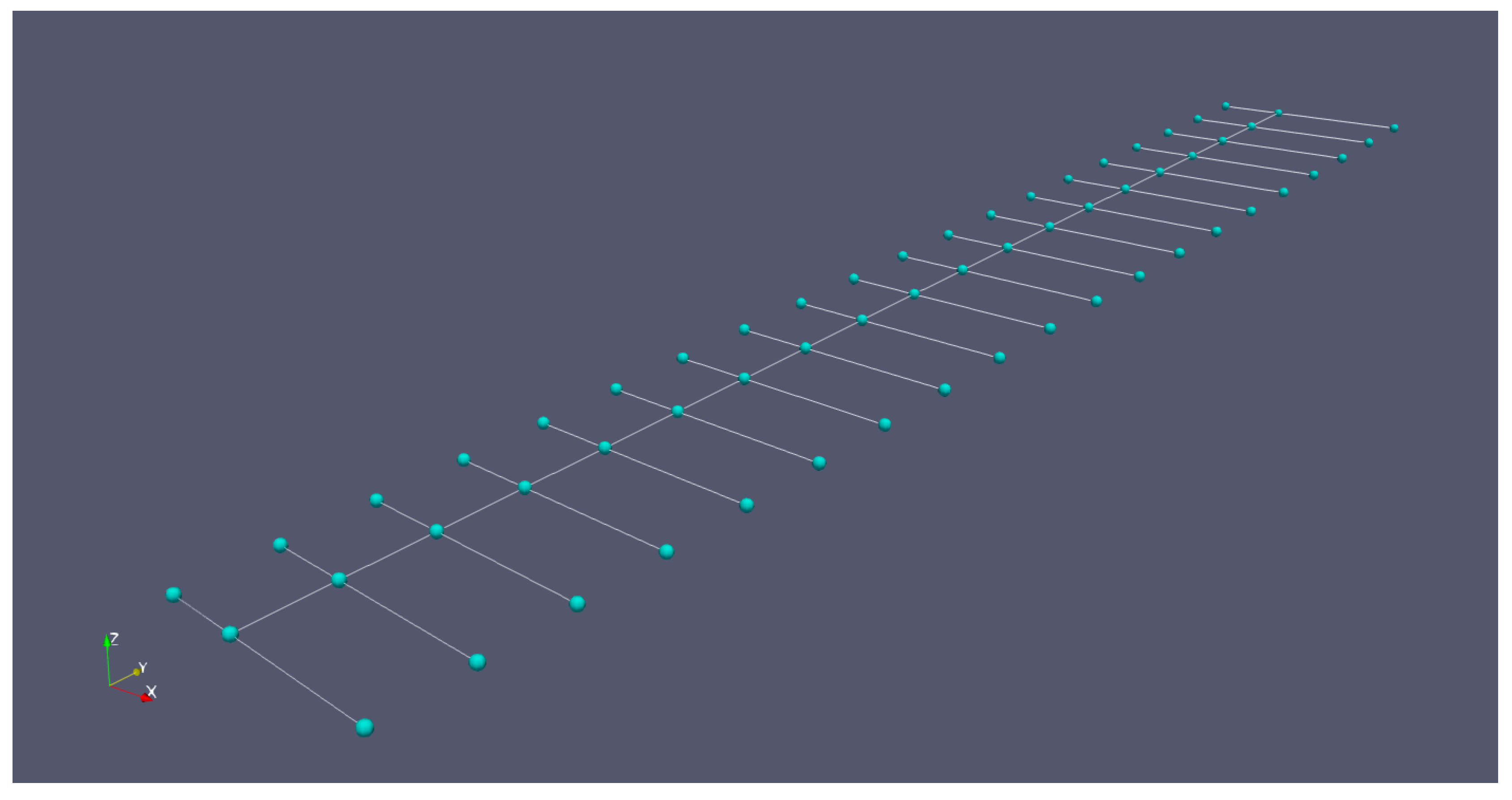
4.1. Structural Model

Following previous works [21], the wing structure is modelled with CBEAM elements and accounts for the distance between inertial and elastic axes; the node lying at the wing root is then clamped (see Figure 1). Further FEM nodes are placed at the leading and trailing edges of the wing and connected to the beam nodes with the rigid elements RBE2, in order to support mapping with the aerodynamic grid (in terms of both structural deformation and aerodynamic load: the latter modifies the former, which changes the airflow boundary condition in turn) according to the closely-spaced rigid diaphragm (CSRD) assumption [57]. For the natural vibration analysis, shear deformation is neglected in order to obtain the Euler–Bernoulli beam model, with PBEAM defining the properties (i.e., inertia and stiffness) of the beam element and SPC1 defining the single-point constraint for the clamped root. Using Nastran’s SOL103 to obtain the structural eigenvalues and eigenvectors, the vibration analysis is performed while selecting Lanczos’ method [58] as available in EIGRL and normalising the modes to unit values of the generalised mass.

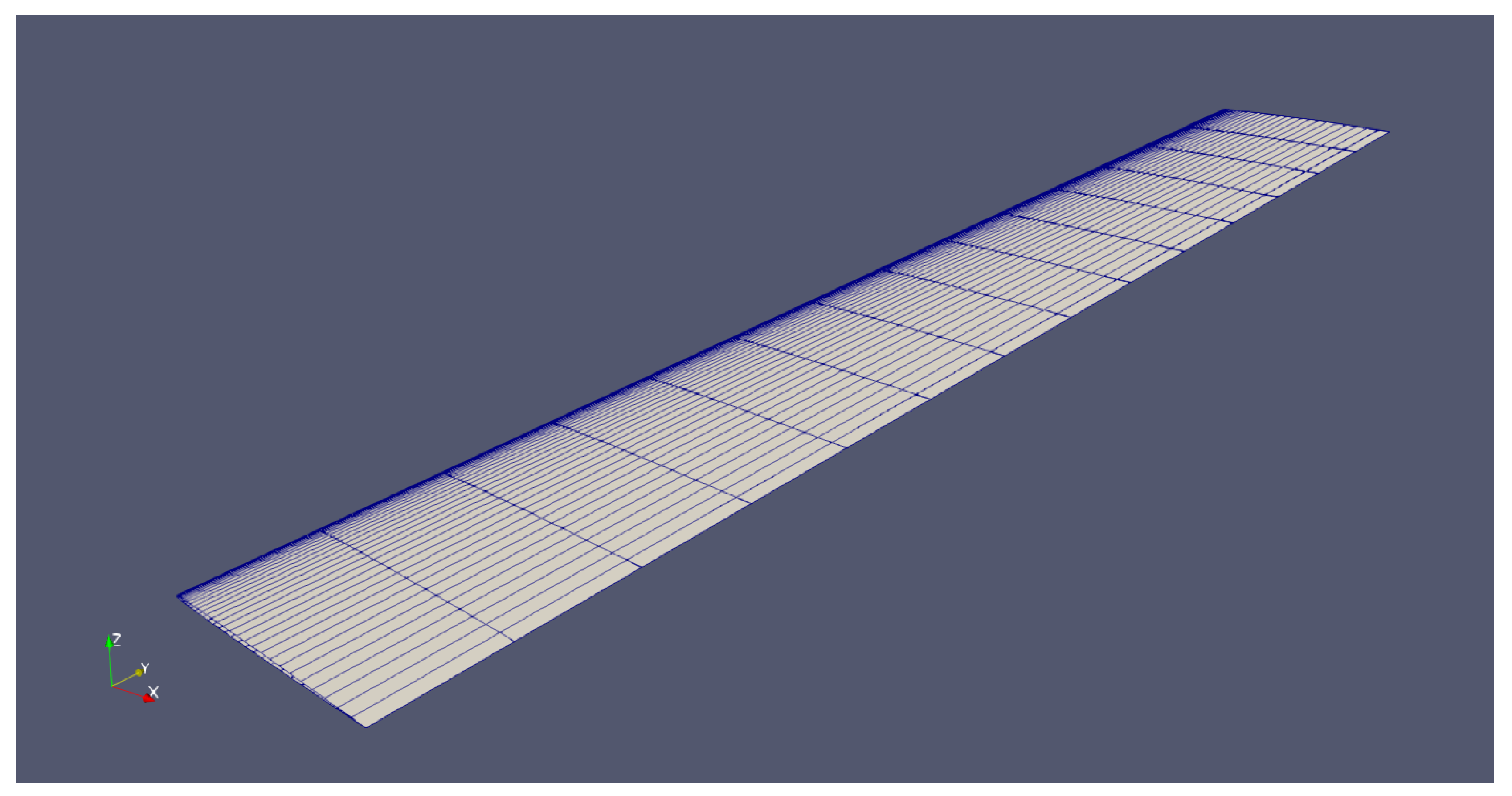
4.2. Aerodynamic Model

Standard flutter prediction methods in the industrial environment are based on aerodynamic panel codes (mostly DLM [59,60]) that idealise wing and empennage as lifting surfaces; if considered, the aircraft fuselage is treated with dedicated elements for non-lifting bodies. The lower computational cost compensates for the lower fidelity of the model; however, the reliability may be increased by correcting the aerodynamic influence coefficients with higher-fidelity data (which are generally not available at the preliminary stage of an MDO process though). Considering small perturbations of an unsteady irrotational flow, the BEM proposed by Morino [55,56] is hereby adopted and consists of an integral representation of the velocity potential at any point of the computational domain in terms of the values on the surface surrounding the aircraft body and wake; the principle of superposition applies. The linear equation of acoustic waves propagation governs the unsteady flow for the case of isentropic compressible fluid and accounts for the finite speed of sound [61], whereas Laplace’s equation is resumed for the case of steady flow by taking advantage of Prandtl–Glauert’s transformation [62]. Green’s function representing a unit-impulsive point source, the theoretical formulation of the boundary value problem for the perturbation potential is then based on Green’s formula [33], with (Neumann-type, generally instationary) non-penetration boundary conditions on the aircraft surface and wake as well as (Dirichlet-type, generally stationary) unperturbed asymptotic conditions far from the latter. Bernoulli’s theorem is linearised to calculate the pressure coefficient and Kutta’s condition is imposed at the trailing edge of lifting surfaces, where the wake detaches and is shed back with the reference airspeed, trailing circulation variations without sustaining any pressure load [37]; its trajectory then represents a streamline at any time and may generally become part of a nonlinear iterative solution where roll-up occurs due to downwash effects, if it is not prescribed a priori (as is in fact typical for most practical applications [53,63], especially when characterised by moderately unsteady flow). Thus, Morino’s BEM is able to deal with arbitrary 3D geometries in a unified manner, reducing the effort of the abstraction process and easing the integration with complex structural models. Although the original theory is valid for arbitrary motion in time or frequency domain, only harmonic oscillations in the frequency domain are here considered as suitable for flutter analysis.
The current implementation of Morino’s BEM is described in previous works [64] and is equivalent to an appropriate combination of doublets (for lifting bodies and wake) and point sources/sinks (for thickness effects and non-lifting bodies). The 3D geometry is approximated with flat quadrilateral panels that follow the local wing surface and the aerodynamic potential is assumed constant over them, with an analytic expression for their mutual induction. Note that similar flow conditions can be modelled by either vortex or doublet distributions and a quadrilateral doublet element is equivalent to a vortex ring placed at the panel edges [65]; higher-order methods have also been formulated in order to improve accuracy and computational efficiency for complex geometries and configurations, but they are more prone to becoming ill-posed and typically not necessary as long as enough quadrilateral panels refine the aerodynamic grid for lower-order methods to capture high pressure gradients while still staying away from ill-conditioning [66]. Through the wake being assumed as flat, rigid and parallel to the free-stream velocity in order to perform rigorous comparisons with Nastran’s DLM and Theodorsen’s theory without loss of generality (in the absence of aircraft fuselage and empennages [67]), a linear system is obtained:
T σ σ k = T ϑ ϑ k ,
where frequency-dependent T σ and T ϑ are the matrices of aerodynamic influence coefficients (AIC), whereas σ k and ϑ k are the aerodynamic potential and normal wash associated with the k-th mode shape of the structural displacement [68], having mapped the latter onto the aerodynamic grid with an effective implementation of the infinite plate spline (IPS) method [69]. The elements Q h k of the generalised aerodynamic forces (GAF) matrix Q ( s ) are then calculated from the work done by the aerodynamic pressure C p due to the k-th mode on the displacement defined by the h-th mode ϕ h for a prescribed range of reduced frequencies [40], namely:
Q h k = i = 1 N ϕ i h · n i A i C p i ( σ k ) ,
where n i and A i are the normal vector and area of the i-th aerodynamic panel, respectively.
The NACA0002 aerofoil [26] is suitably adopted to obtain a baseline 3D representation of Loring’s wing surface (see Figure 2); this particular choice of thin symmetric aerofoil is consistent with the original work with no loss of generality, as the parametric sensitivity of the aeroelastic stability boundary with respect to aerofoil thickness was already found to be poor for small perturbations of subsonic potential flow (i.e., in the absence of strong shock waves and/or significant flow separation) [70].

4.3. Aeroelastic Model

After obtaining the natural vibration modes, the GAF are computed with Morino’s BEM, and the continuation method [50] is used to solve the aeroelastic stability eigenproblem and trace the root locus. In order to avoid its costly re-computation during the stability analysis, the GAF matrix is approximated by a rational expression in which the non-linear dependency on the complex reduced frequency s appears explicitly. Here the matrix fraction approach (MFA) [71] is used and preferred to the rational function approximation (RFA) [72], since the former exhibits higher accuracy than the latter for the same number of poles [73]; yet, both methods provide the analytical continuation of the GAF for complex reduced frequency, increasing the accuracy of damped solutions with respect to the p k method. According to MFA, the GAF matrix is expressed as fraction of matrix polynomials:
Q i = 0 M + 2 N i s i i = 0 M D i s i 1 ,
and the accuracy of the approximation increases with increasing the number of poles M, which is equal to the size of the state-space system [74]; in particular, three poles have been used in this proof-of-concept work. The approximation matrices D i and N i are both obtained by solving a least-square problem in which the distance from the GAF samples Q ( ik ) is minimised.
The continuation method hereby adopted provides a straightforward and efficient tracking technique without using any correlation function, such as the modal assurance criterion (MAC) [75]. For this reason, the method is rather insensitive to the number of poles used for the aerodynamic finite-state approximation and is able to distinguish between actual and artificial aerodynamic states by construction. In the continuation method, the aeroelastic equations are differentiated with respect to the free-stream airspeed, thereby resulting in a system of ODEs which are solved with a predictor–corrector integration schema starting from an initial airspeed value for which a true solution is known (e.g., the natural vibration frequencies for U = 0 ).
For validation purposes, flutter analysis is also carried out with Nastran’s DLM directly: a flat plate aligned with the free-stream is used as lifting surface and the aerodynamic panels are defined with CAERO1 and PAERO1 cards; the distribution and number of such panels follow established guidelines and convergence studies (see Appendix B). The mode shapes are mapped onto the aerodynamic grid with the IPS method [76] using the SPLINE1 card and the GAF matrix is then generated for sixteen reduced frequencies specified in the MKAERO1 card, suitably ranging from k = 0 to k = 1 (with logarithmic-like spacing) as per literature studies and common practice [53,63]; a cubic spline is then exploited to interpolate the GAF therein. For the dynamic aeroelastic stability analysis, the p k method as available in the FLUTTER card is used: the aerodynamic damping is approximated as the imaginary part of the GAF matrix computed for (undamped) harmonic motion, limiting results’ accuracy to the case of lightly damped aeroelastic solutions [12]. The p k approximation of the aeroelastic eigenproblem [77] is then solved for all the free-stream speed values defined in the FLFACT card, according to the reference length and air density specified in the AERO card. After damping ratios are obtained in the given speed range for all modes, the (undamped) flutter point is determined by linear interpolation.

4.4. Aero-Structural Parametric Derivatives

To calculate the sensitivity of the flutter boundary with respect to any aero-structural parameter, the derivatives of the aeroelastic matrices are also necessary in the first place. In particular, the derivatives of structural eigenvalues and eigenvectors with respect to structural parameters, such as wing material properties (e.g., density or elastic modulus) and element properties (e.g., moments of inertia or distance between elastic and inertia axis), are obtained with Nastran SOL200. The design variable label and initial value are defined with the DESVAR card, which is connected to the relative bulk data entry by DVMREL1 or DVPREL1 cards for material or element properties, respectively; derivatives are hence computed for the structural responses defined by DRESP1 cards, which are the first n structural eigenvalues and eigenvectors.
The GAF matrix is differentiated with respect to both reduced frequency and design variables: according to MFA, the finite-state approximation allows the analytic differentiation with respect to the complex reduced frequency s, whereas the method presented in previous works [73] was used for the derivatives with respect to the design variables p . In particular, by defining the functions P σ k , p and R σ k , p as:
P = Q h k σ k , p , R = T σ σ k T ϑ ϑ k ,
a sub-differentiation process is set up, and depending on the number of design variables and mode shapes to be considered [11], the derivatives may be obtained by either a direct approach:
d P d p = P p + P σ d σ d p , R σ d σ d p = R p ,
or an adjoint approach:
d P d p = P p + Λ R p , R σ T Λ = P σ T .
In computing the partial derivatives, it is important to note that the imaginary component is introduced only by the normal wash ϑ and the wake’s influence coefficients inside matrix T σ ; therefore, the partial derivatives of the steady (real) contribution to the GAF are computed via complex step [78] and the partial derivatives of the unsteady (complex) contribution are then analytically assembled.

5. Results and Discussion

Loring’s uniform slender thin wing [25] is hereby considered, as both experimental wind-tunnel data and numerical results assuming two-dimensional incompressible potential flow are available and all results can hence be explained from both physical and mathematical standpoints; moreover, this fundamental benchmark embeds the full complexity of the aeroelastic problem without introducing detrimental uncertainties. The wing’s chord is 0.305 m and the semi-span is 2.057 m, giving an aspect ratio 13.5 . The inertial axis lays at 42.3 % of the chord, with mass 8.05 kg/m and mass moment of inertia 0.0471 kg·m. The wing root is clamped at the elastic axis, with flexural stiffness 677.3 N·m 2 and torsional stiffness 1018.9 N·m 2 placed at 30 % of the chord.
The coupled natural vibration frequencies of the first bending and torsion modes were observed at 1.29 and 18.1 Hz, respectively; that of the second bending mode was detected in between at 7.7 Hz. With a fluid density 1.11 kg/m 3 , the flutter speed and frequency were experienced at 90.3 m/s and 10.2 Hz, which give a reduced frequency around 0.11 ; the subsonic flow may then be considered as moderately unsteady. A Euler–Bernoulli beam model calculated the first three coupled vibration frequencies as 1.29, 7.65 and 17.98 Hz; once coupled with two-dimensional unsteady aerodynamics for a flat plate using standard strip theory, flutter was predicted at 90.7 m/s and 9.2 Hz with good accuracy.
In order to elaborate on the literature results and visualise the flutter mechanism, the aeroelastic stability analysis of Loring’s wings is first performed with the same assumptions as in the original publication and the approach here described in the Problem Formulation; the p k method (with Theodorsen’s exact function [35]) has consistently been used and results have been cross-verified against the state-space representation (with a common two-term RFA of Theodorsen’s function) [21]. By employing the first two bending modes and the first torsion mode, the respective coupled vibration frequencies are calculated as 1.21, 7.59 and 17.91 Hz; once still coupled with two-dimensional unsteady aerodynamics for a flat plate using standard strip theory, flutter is consistently predicted at 91.15 m/s and 9.2 Hz (which is indeed an excellent approximation, as confirmed by a modal convergence study up to the first three bending and torsion modes). The evolution of the aeroelastic system’s eigenvalues is presented in Figure 3 and confirms static divergence to arise well beyond dynamic flutter (i.e., U d > > U f ).
Due to the remarkable agreement between measurements and simulations, the assumptions of slender beam structure and two-dimensional incompressible potential flow in the latter are hence deemed justified. Note that the instability mechanism involves second bending and first torsion modes directly, but the first bending mode is indirectly essential for their coupling to occur before that between first bending and first torsion modes (see Appendix A).

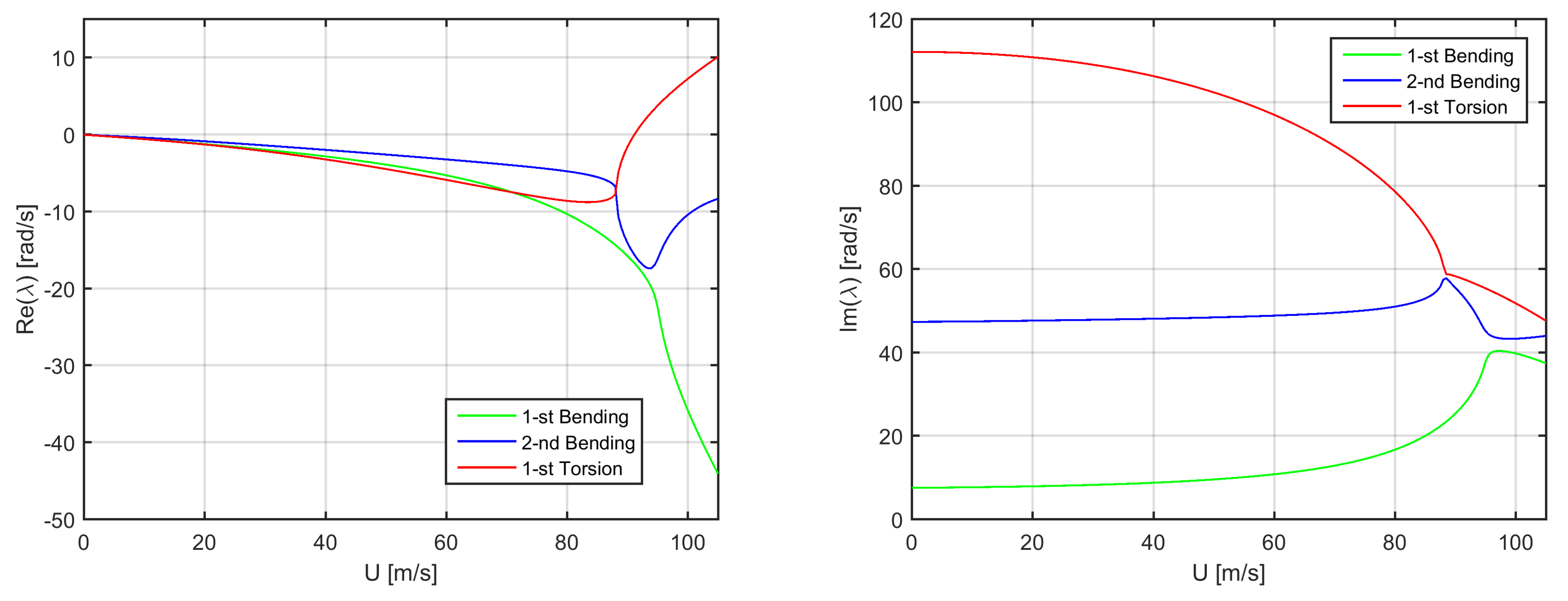
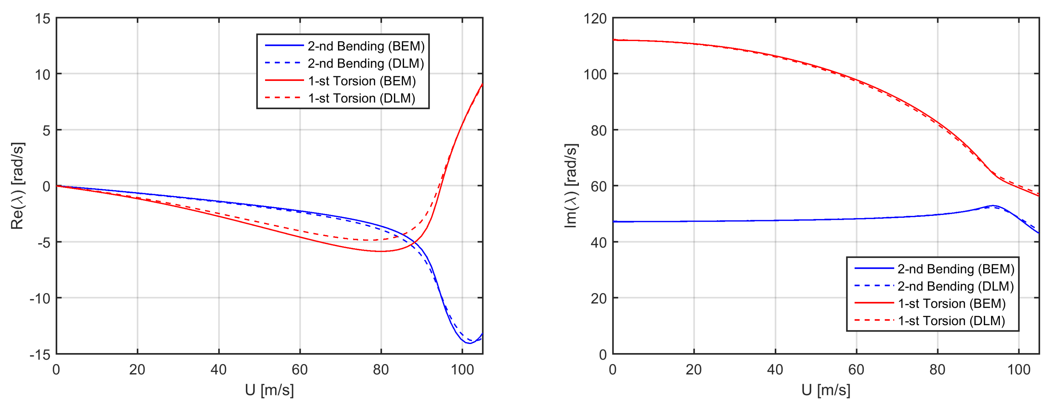
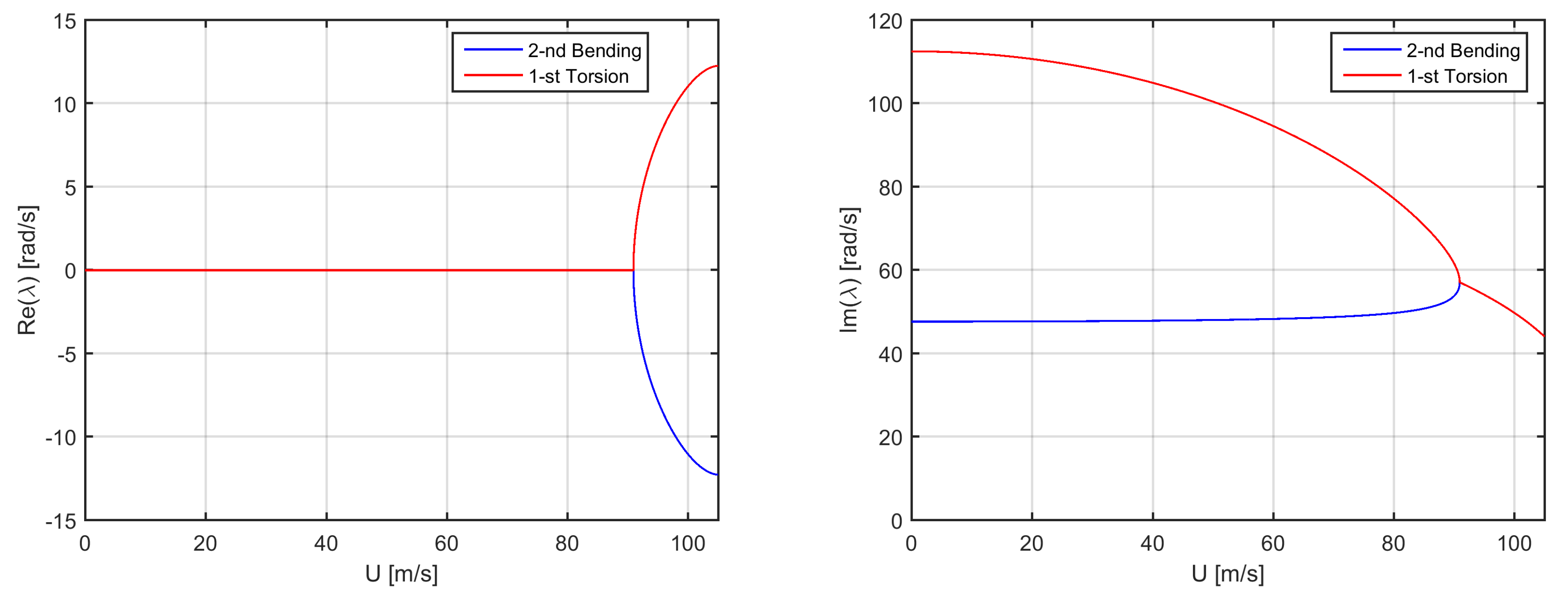
5.1. Aeroelastic Analyses

The aeroelastic stability of Loring’s wing is investigated and compared using the proposed lower and higher-fidelity models, while still assuming incompressible flow. The analyses encompass parametric variations of the aero-structural properties, quantifying their effects on the aeroelastic stability boundary and critically assessing the differences in the multifidelity results from both theoretical and computational perspectives, for possible practical applications in airplane design and optimisation adopting hybrid strategies.
Figure 4 shows the aeroelastic stability analysis from the higher-fidelity model, focusing on the same flutter mechanism as found earlier: the first torsion mode becoming unstable and extracting energy from the airflow through the coupled second bending mode, flutter is found at 94.77 m/s and 10.04 Hz in excellent agreement with the experimental results and exhibits a slightly higher vibration frequency than the theoretical one. The aeroelastic stability analysis performed with Nastran and its embedded DLM for the flat wing is also presented and confirms the higher-fidelity results based on Morino’s BEM with NACA0002 aerofoil, flutter being found at 94.44 m/s and 10.38 Hz. Note that both sets of code share the same structural model, and the coupled natural vibration frequencies in the void are 1.21, 7.55 and 21.03 Hz for the first three bending modes, whereas it is 17.88 Hz for the first torsion mode; these first four modes have been used in all analyses (see Appendix B). As expected from the wing aspect ratio being relatively large, three-dimensional downwash effects are actually moderate and the (beneficial) steady ones on the (attenuated) airload distribution are roughly compensated by the (detrimental) unsteady ones on the (accelerated) airload evolution [21]; thus, the flutter speed is just slightly higher than that predicted assuming unsteady two-dimensional flow.
Still focusing on the flutter mechanism, Figure 5 then shows the aeroelastic stability analysis from the lower-fidelity model: despite its inherent simplicity, the latter predicts flutter quite accurately at 92.1 m/s and 9.09 Hz, thereby proving the effectiveness of such an idealisation (analogous stability diagrams have indeed been obtained by retaining only steady aerodynamic terms in the higher-fidelity model, for cross-verification purposes). The coupled natural vibration frequencies in the void are 1.21 and 7.59 Hz for the two bending modes, and 17.91 Hz for the torsion mode, in excellent agreement with the higher-fidelity ones. The aeroelastic response is then metastable until the first instability occurs, as no damping is provided by either the elastic structure or static aerodynamics; to this respect, it is worth mentioning that the lift-derivative correction for the steady three-dimensional downwash (which tends to increase the flutter speed, by providing lower airload) incidentally compensates the lack of aerodynamic lag (which tends to decrease the flutter speed, by neglecting wake inflow). Note that, although the flutter reduced-frequency is rather high for steady aerodynamics to be rigorously applicable, the latter was still adopted in order to exacerbate the difference between lower and higher-fidelity models and stress the multilevel approach for more general conclusions.

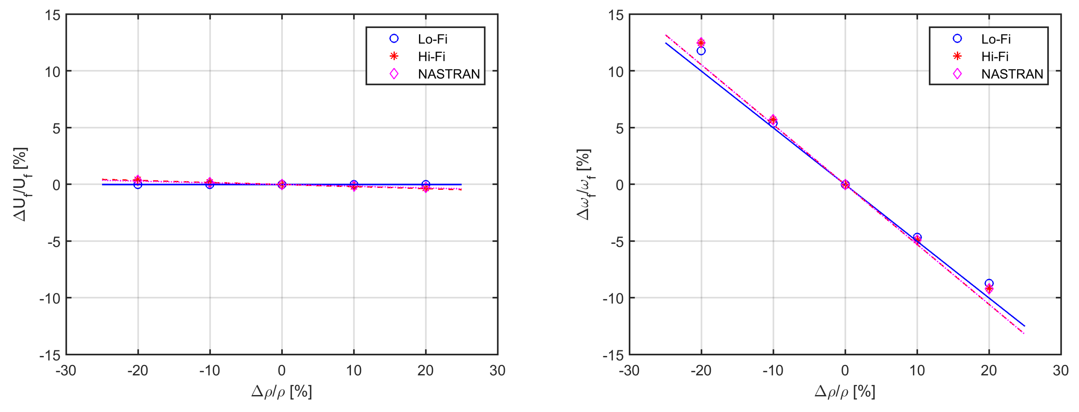
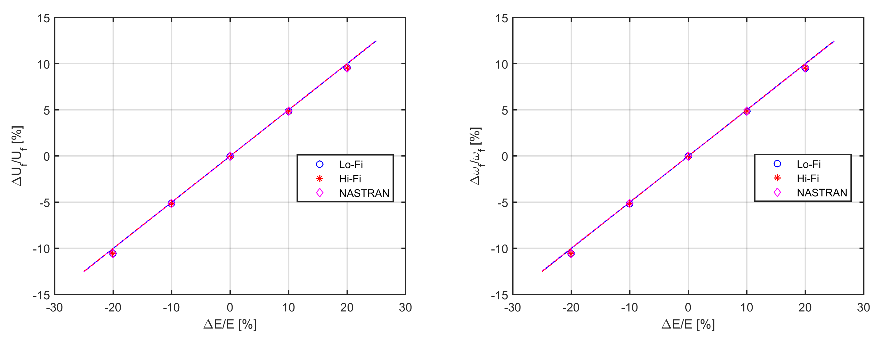
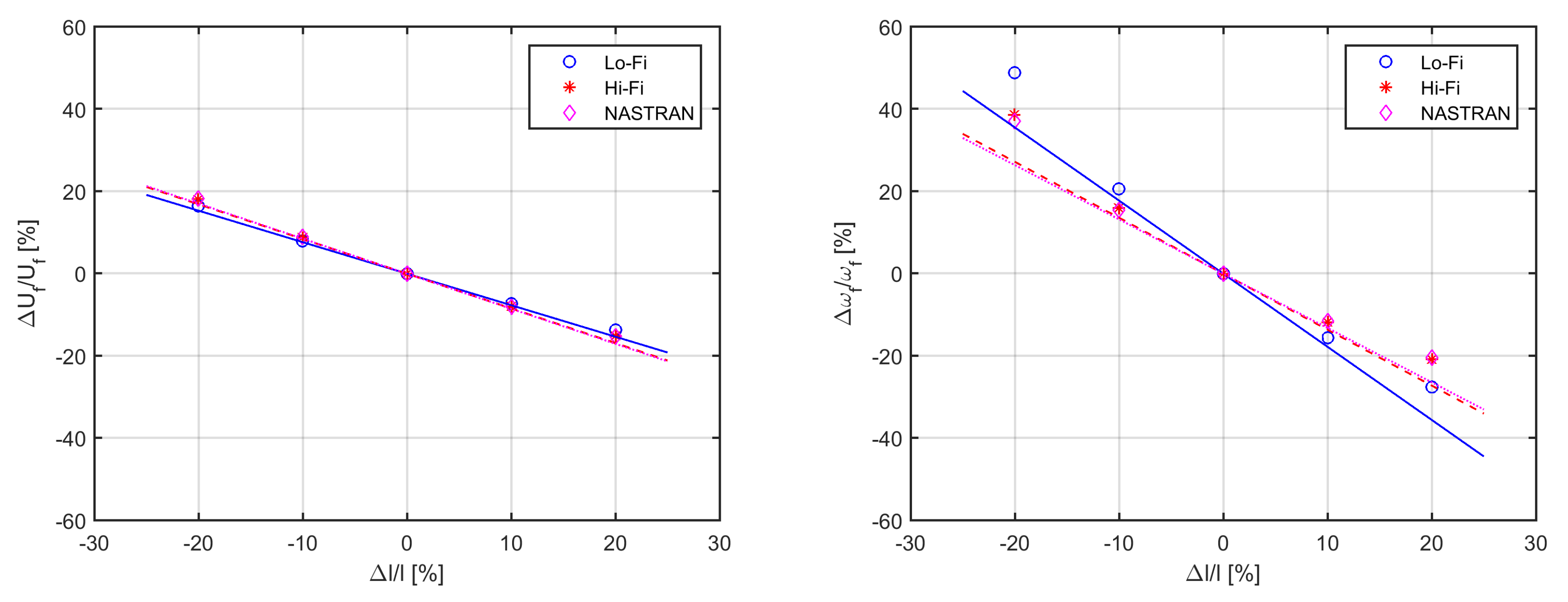
5.2. Sensitivity Study

Following previous studies on the aeroelastic stability boundary of slender cantilever wings and its sensitivity [27,28], linear FSI models give nonlinear flutter trends as relevant aero-structural parameters are perturbed. The reciprocal positions of aerodynamic, elastic and inertial axes being often constrained by the available space inside the wing as well as the chosen structural layout and systems arrangement, the flutter point’s sensitivity to the wing’s structural properties is individually explored by changing its material density ρ m (which scales m and μ ) and elastic modulus E (which scales E I and G J ), whereas varying the wing’s semi-span l (which modifies the lift coefficient derivative C l / α ) alters its geometry and affects both structural and aerodynamic properties at the same time.
From Figure 6, it can be seen that changing the wing’s material density alters all natural frequencies through the inertial properties and hence the flutter frequency, but has marginal/no influence on the flutter speed; all symbols give the actual nonlinear percentage variation of the flutter point, whereas all lines with corresponding colour draw its normalised linear prediction. In particular, a 1 % increment in the material density causes about a 0.5 % decrement in the flutter frequency; the negligible variation of the flutter speed is confirmed by previous works [27] as being due to the (small) beneficial effect of an increase in sectional mass being compensated by an (almost) equal and opposite detrimental effect of an increase in mass moment of inertia. This outcome may indeed help while minimising the aeroplane weight, as reducing the material density does not significantly affect the present flutter boundary due to wing bending–torsion instability (especially in the absence of lumped masses). However, it shall be recalled that varying the wing inertia might cause other types of aero-structural instabilities to arise at the aircraft level due to modal coalescence, and monitoring the variation of the flutter frequency is then important to preventing potential resonance. It is also worth mentioning that the small higher-fidelity effect on the flutter speed is due to the unsteady airload being frequency dependent through the lift-deficiency function and the related aerodynamic lag.
As per Figure 7, changing the wing’s material elastic modulus alters all natural frequencies through the stiffness properties and hence the flutter speed and frequency; in particular, a 1 % increment in the elastic modulus induces about a 0.5 % increment in all the latter, leaving the flutter reduced frequency practically unchanged. This outcome is quantitatively confirmed by previous works [27] as being due to the detrimental effect of an increase in flexural stiffness being much lower than the beneficial effect of an increase in torsional stiffness. The striking agreement between lower and higher-fidelity results is mostly driven by the respective structural models being equivalent (as seen from the close agreement between the natural vibration frequencies), while the different aerodynamics play a minor role (as the airflow is moderately unsteady). The quasi-linear trend of the percentage variations reveals a rather large confidence interval for the normalised sensitivity; however, the dimensional counterpart of the latter to be used by optimisation routines follows a highly nonlinear pattern (note that the explicit lower-fidelity expression given in Appendix A for the torsional static divergence speed provides a straightforward theoretical check).
Finally, Figure 8 shows that changing the wing semispan has a large effect on the stability boundary through the stiffness properties as well as the aerodynamic loads and hence on the flutter speed and frequency. In particular, a 1 % increment in the wing semispan induces about a 0.8 % decrement in the critical speeds and about a 1.6 % decrement in the flutter frequency; note that analogous trends for the variations and orders of magnitude for the sensitivities were obtained in previous studies on similar slender wings [28], as a qualitative means of validation. Lower and higher-fidelity results are still in very good agreement and differences are mainly due to unsteady downwash effect, as the aspect ratio of the wing changes considerably with the span and so does the sectional airload.
For the sake of completeness, it is worth mentioning that variations and sensitivities of the divergence speed (see Appendix A) with respect to the same aero-structural parameters considered above were consistently found to have trends and orders of magnitude very close to those pertaining the flutter speed. In particular, it is observed that changing the wing’s geometry has a much larger impact on the flutter boundary than changing the material properties (especially density); this is particularly true for the flutter frequency, the variations of which exhibit a more significant nonlinear behaviour and local curvature.
Due to the sufficient mutual separation of the natural vibration modes, it is also worth stressing that the instability mechanism did not change across the parametric variations, and the derivatives of the flutter stability boundary have accurately been calculated by the lower-fidelity model at a (marginal) fraction of the computational complexity and costs. In particular, semi-analytical solutions drastically reduced the latter, being almost instantaneous and demanding minimal pre- and post-processing (if any at all) while granting an enhanced theoretical understanding. Thus, the healthy combination of lower and higher-fidelity models enables efficient multidisciplinary exploration of a large design variable space for innovative aeroplane concepts and configurations; further numerical savings may still be obtained by exploiting reliable surrogate models for the higher-fidelity solutions, with an effective synthesis of the underlying complexity [20].

6. Conclusions

Within the context of aircraft multidisciplinary design and optimisation, a comparative sensitivity study for the bending–torsion flutter instability of flexible aircraft wings in subsonic flow has been presented. Analytical models and numerical tools with different complexities and fidelities have been used, in view of possible practical applications exploiting multilevel approaches within the conceptual and preliminary MDO phases. Parametric studies have been performed where the effects of varying the wing’s aero-structural properties on the aeroelastic stability boundary have been quantified and critically assessed from both theoretical and computational perspectives. When the natural vibration modes of the wing are well separated from all other natural vibration modes of the aircraft and the aeroelastic instability mechanism does not change in nature, an efficient hybrid strategy is then recommended where the flutter analysis is performed using higher-fidelity approaches, whereas the sensitivity analysis of the flutter boundary is performed using lower-fidelity approaches, thereby improving theoretical understanding and reducing computational costs while retaining accuracy. Future works are encouraged to investigate additional effects (e.g., wing sweep and flow compressibility) and increased complexity (e.g., presence of a control surface) or perform the full MDO of a flexible aircraft wing, effectively exploiting the proposed multifidelity strategy.

Author Contributions

M.B. derived the analytical model and results; F.T. performed the numerical simulations; the authors then wrote the respective parts of the manuscript. All authors have read and agreed to the published version of the manuscript.

Funding

This research received no external funding.

Acknowledgments

The authors would like to thank Ranjan Banerjee at City University of London and Rakesh Kapania at Virginia Polytechnic Institute and State University for the precious insights into their previous works.

Conflicts of Interest

The authors declare no conflict of interest.

Abbreviations

Symbols
Aaerodynamic panel area
csection chord
C l section lift
C l / α section lift derivative
C L / α wing lift derivative
C p pressure coefficient
C T Theodorsen’s function
C generalised damping matrix
D aerodynamic approximation matrix (fraction denominator)
esemiperimeter-to-span ratio
Esection Young’s elastic modulus
fcross-projection of first bending and first torsion modes
F generalised load vector
gcross-projection of second bending and first torsion modes
Gsection shear elastic modulus
hsection flexural (plunge) displacement
H n 2 Hankel’s functions of the second type and n-th order
Isection flexural area moments of inertia
Jsection torsional area moments of inertia
kreduced frequency
kequivalent spring stiffness
[ K ] generalised stiffness matrix
lwing semi-span
Δ L section aerodynamic force
msection mass
Δ M section aerodynamic moment
[ M ] generalised mass matrix
n aerodynamic panel normal vector
N aerodynamic approximation matrix (fraction numerator)
pdesign parameter
Q generalised aerodynamic forces matrix
rsquared ratio of second and first flexural vibration frequencies
scomplex reduced frequency
[ S ] system matrix
ttime
T aerodynamic influence coefficients matrix
u eigenvector
Uhorizontal airspeed
Vvertical airspeed
xchordwise coordinate
yspanwise coordinate
wsection vertical displacement
Greek
α angle of attack
χ generalised coordinates
ϵ aerofoil thickness ratio
ϕ natural vibration mode shape
γ flexural natural vibration constant
η wing aspect ratio
κ aerodynamic load scaling function
λ eigenvalue
μ section mass moment of inertia
ν torsional natural vibration constant
θ section torsional (pitch) displacement
ϑ normal wash matrix
ρ air density
ρ m material density
σ aerodynamic potential matrix
τ reduced time
ω natural vibration frequency
Subscripts
Aaerodynamic
ccritical
fflutter
ddivergence
hflexural
Sstructural
θ torsional
Acronyms
ACaerodynamic centre
AICaerodynamic influence coefficient
BEMboundary element method
CFDcomputational fluid dynamics
CGcentre of gravity
CPcontrol point
CSRDclosely-spaced rigid diaphragm
DLMdoublet lattice method
EAelastic axis
FEMfinite element method
FSIfluid-structure interaction
GAFgeneralised aerodynamic forces
IPSinfinite plate spline
MACmodal assurance criterion
MCmid-chord
MDOmultidisciplinary design and optimisation
MFAmatrix fraction approach
MSTmodified strip theory
ODEordinary differential equation
PDEpartial differential equation
QSTquasi-steady theory
RFArational function approximation
ROMreduced order model
SSTstandard strip theory
TSTtuned strip theory

Appendix A. Aeroelastic Stability of the Typical Section with Steady Aerodynamics

Providing full control on the results with respect to the specific assumptions of the methods and tools employed for the analysis, theoretical formulations grant a clear and complete overview of the problem which is essential for any engineering application. Although inherently limited in their general capabilities, analytical solutions then offer a wealth of qualitative information and quantitative details as well as fundamental insights and rigorous validation for both educational and practical purposes.
Considering a single mode for the wing bending and torsion, respectively, the aeroelastic equations for the Typical Section with steady aerodynamics read [79]:
m h ¨ x C G f θ ¨ + k h h = ρ 2 U 2 c C L / α f θ ,
μ θ ¨ m x C G h ¨ x C G f θ ¨ + k θ θ = ρ 2 U 2 x A C c C L / α θ ,
where f 1 for two-dimensional aerofoils [12], with ϕ h 1 and ϕ θ 1 . By neglecting the aerodynamic load, the coupled bending and torsion natural vibration frequencies are explicitly obtained as:
F 4 ω v 4 F 2 ω v 2 + F 0 = 0 , ω v = 1 2 F 4 F 2 ± F 2 2 4 F 4 F 0 ,
F 0 = 1 , F 2 = μ μ + m x C G 2 1 f 2 ω θ 2 + 1 + m μ x C G 2 ω h 2 , F 4 = μ ω h 2 ω θ 2 μ + m x C G 2 1 f 2 ,
where the uncoupled counterparts are resumed whenever inertial and elastic axes coincide (i.e., with x C G = 0 ). Otherwise, the characteristic equation for the flutter determinant provides with the metastable boundary and gives the flutter frequency as:
P 4 ω f 4 P 2 ω f 2 + P 0 = 0 , ω f = 1 2 P 4 P 2 ± P 2 2 4 P 4 P 0 ,
and setting the inner radical discriminant equal to zero then gives the flutter speed as:
D 4 U f 4 + D 2 U f 2 + D 0 = 0 , U f = 1 ρ D 4 D 2 ± D 2 2 4 D 4 D 0 ,
where the sign before the inner radical shall provide with the smallest positive real value; finally, note that setting both ω f and P 0 equal to zero provides with the torsional static divergence speed. In particular, when the aerodynamic centre is ahead of the elastic axis (i.e., with x A C < 0 ), the latter explicitly reads:
U d = 2 k θ ρ x A C c C L / α ,
regardless the bending stiffness; when the elastic axis is ahead of the inertial axis (i.e., with x C G > 0 ), the flutter condition is given as:
U f = 1 ρ D 4 D 2 2 4 D 4 D 0 D 2 , ω f = P 2 2 P 4 ,
where all coefficients are analytical functions of the aero-structural parameters, namely:
P 0 = k h k θ + ρ 2 U 2 x A C c C L / α ,
P 2 = m k θ + ρ 2 U 2 x A C x C G f 2 c C L / α + k h μ + m x C G 2 ,
P 4 = m μ + m x C G 2 1 f 2 ,
D 0 = m k θ + k h μ + m x C G 2 2 4 m μ + m x C G 2 1 f 2 k h k θ ,
D 2 = 2 m x A C x C G f 2 k θ m + k h μ + m x C G 2 2 μ + m x C G 2 1 f 2 x A C k h c C L / α ,
D 4 = m x A C x C G f 2 c C L / α 2 .
The formulas above were implemented and compared with literature results for the stability boundary of a Typical Section assuming standard strip theory (SST) with steady aerodynamics [12,79]: exact agreement was always found and provided rigorous validation, also with respect to the relative root locus. The same formulas have then been used to investigate the stability boundary of Loring’s wing Typical Section when either the first or the second bending mode is coupled with the first torsion mode, employing tuned strip theory (TST) with steady aerodynamics [21]. Without accounting for the modal cross-projection (i.e., f 1 for a “pitch & plunge” apparatus), flutter is calculated at 106.5 m/s and 4.32 Hz in the former case whereas at 73.9 m/s and 11.28 Hz in the latter case; when the modal cross-projection is considered (i.e., f < 1 for a slender beam), flutter is calculated at 109.7 m/s and 4.28 Hz in the former case whereas at 139.2 m/s and 9.60 Hz in the latter case. The static divergence speed pertains the torsion mode only and is found at 210.2 m/s, regardless the bending modes and their cross-projections.
A direct comparison with the low-fidelity results hence reveals that the interaction between bending and torsion modes as well as their cross-projections are essential to reproduce the correct behaviour of the flutter mechanism, where the coalescence between first bending mode and torsion mode drives that between second bending mode and the latter (which have closer natural vibration frequencies) to occur earlier.

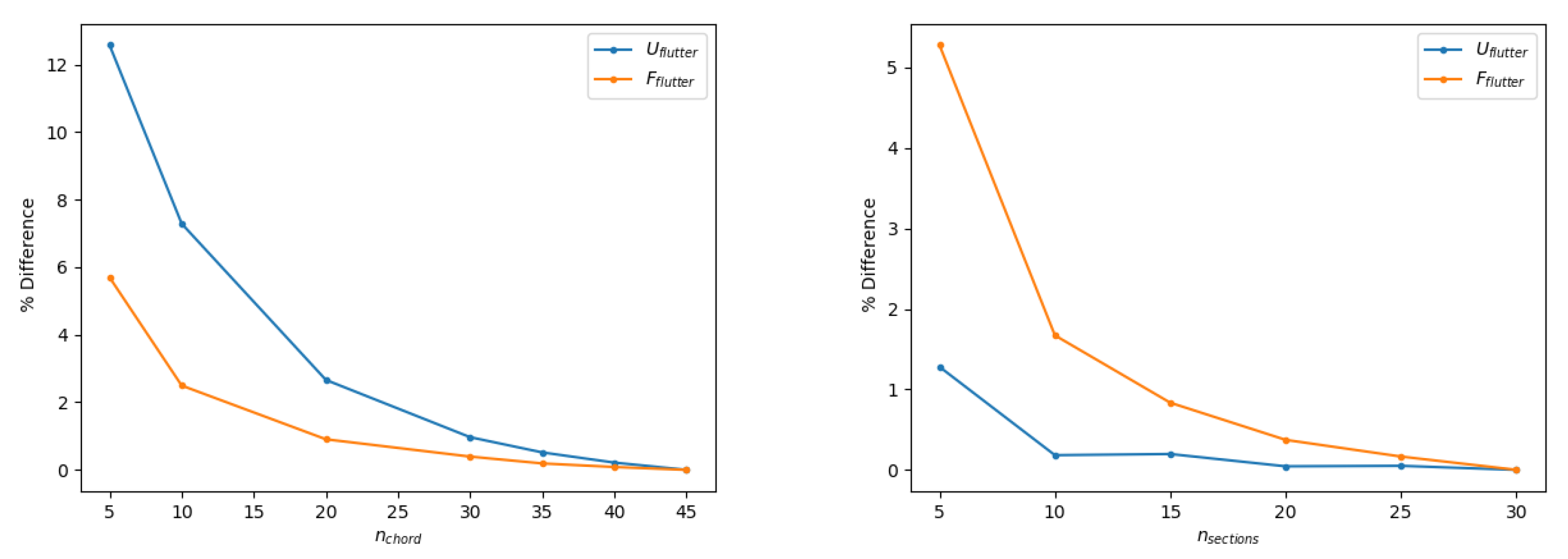
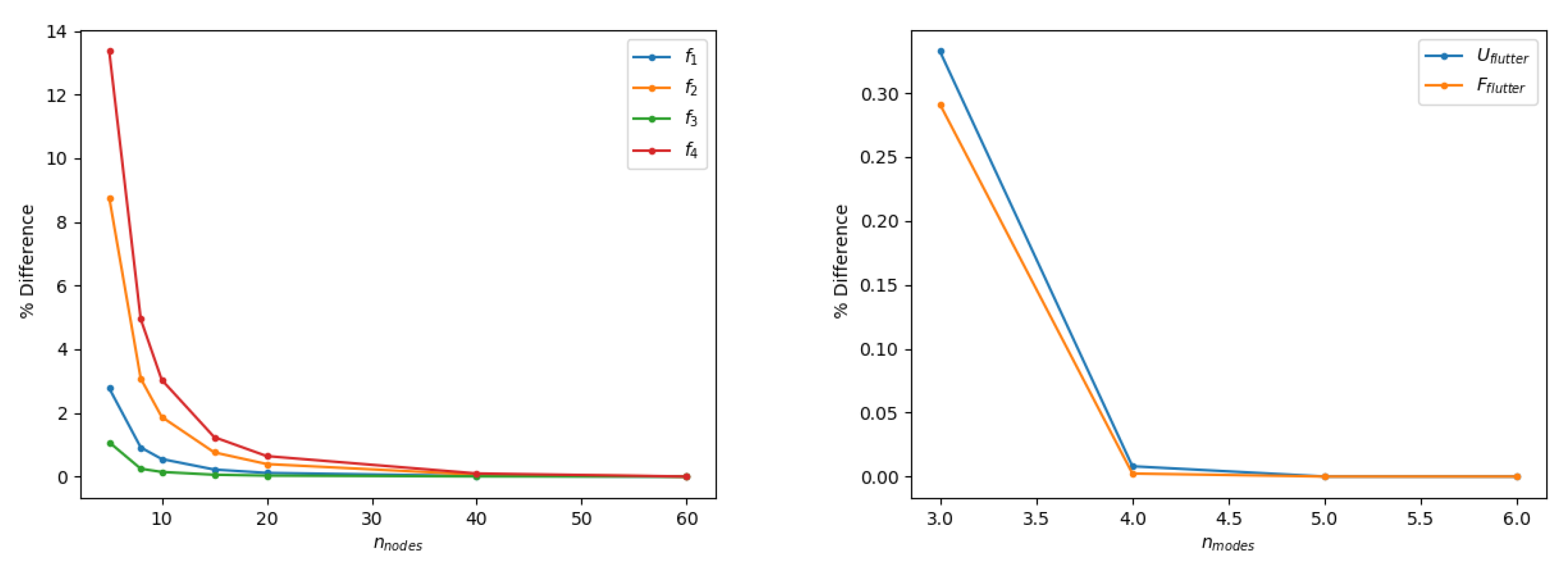
Appendix B. Higher-Fidelity Model Results Convergence Study

The number of elements for the structural and aerodynamic models was defined according to rigorous convergence studies. Following Nastran’s best practice [80] with k m a x = 1 the maximum reduced frequency employed in the aeroelastic analysis, fifteen DLM panels have uniformly been distributed along the wing chord. When adopting Morino’s BEM, thirty aerodynamic panels were symmetrically placed along both upper and lower aerofoil surfaces according to the convergence study in Figure A1 (left), with a suitable refinement around the leading edge in order to capture high pressure gradients. The number of aerodynamic panels in the span-wise direction was determined according to another convergence study shown in Figure A1 (right) and all higher-fidelity results presented in this work were obtained with fifteen panels strips uniformly distributed along the wing span, since sufficient to grant a relative error below 1 % for both flutter speed and flutter frequency. Following convergence studies in previous works [37,64], the wake extends for a hundred chords behind the wing and is modelled with a hundred rows of shed panels, the length of which is cubically increased with increasing their distance from the trailing edge. Figure A2 (left) shows the indicial lift-deficiency function Φ ( τ ) (which represents the equivalent of the complex lift-deficiency function C T in the reduced-time domain τ ) from a unit step in angle of attack, whereas Figure A2 (right) depicts the normalised distribution of the steady circulation κ ( y ) (which represents the ratio between the sectional circulation in three- and two-dimensional flow within the framework of modified strip theory, MST [13]); note that the unsteady lift development approaches quasi-steady theory (QST) asymptotically. These results also justify the assumption of two-dimensional flow for the lower-fidelity model, within the framework of TST [21] (to this respect, it is worth mentioning the higher-fidelity lift coefficient derivative of the wing is obtained as C L / α = 5.25 , in excellent agreement with the lower-fidelity analytical estimation C L / α = 5.21 ).
Figure A1. Flutter speed and frequency varying the number of aerodynamic panels along the wing chord (left) and span (right).
Aerospace 07 00161 g0a1
Figure A2. Indicial lift-evolution function from a step-change in the angle of attack (left), spanwise lift-decay function (right) for Loring’s wing in incompressible flow.
Aerospace 07 00161 g0a2
Figure A3 (left) then shows the evolution of the natural vibration frequencies percentage error with varying the number of FEM nodes of the structural beam; the value obtained with the most dense grid is used as reference to compute the plotted error. The first four natural vibration frequencies exhibit a good convergence behaviour, with the third one (i.e., the first torsional mode) almost insensitive to the number of nodes. All higher-fidelity results presented in this work were hence obtained with 20 nodes uniformly distributed along the wing span, since sufficient to grant a relative error below 2 % . Finally, Figure A3 (right) shows that employing the first four natural vibration modes granted convergence of both flutter speed and flutter frequency.
Figure A3. Natural vibration frequencies varying the number of FEM nodes along the wing span (left), flutter speed and frequency varying the number of natural vibration modes employed in the aeroelastic stability analysis (right).
Aerospace 07 00161 g0a3

References

  1. Alexandrov, N.; Hussaini, M. Multidisciplinary Design Optimization: State of the Art; SIAM: Philadelphia, PA, USA, 1997. [Google Scholar]
  2. Martins, J.; Lambe, A. Multidisciplinary Design Optimization: A Survey of Architectures. AIAA J. 2013, 51, 2049–2075. [Google Scholar] [CrossRef] [Green Version]
  3. Quarteroni, A.; Rozza, G. Reduced Order Methods for Modeling and Computational Reduction; Springer International Publishing: Cham, Switzerland, 2014. [Google Scholar]
  4. Qu, Z. Model Order Reduction Techniques with Applications in Finite Element Analysis; Springer: London, UK, 2004. [Google Scholar]
  5. Ghoreyshi, M.; Jirasek, A.; Cummings, R. Reduced Order Unsteady Aerodynamic Modeling for Stability and Control Analysis Using Computational Fluid Dynamics. Prog. Aerosp. Sci. 2014, 71, 167–217. [Google Scholar] [CrossRef] [Green Version]
  6. Livne, E. Integrated Aeroservoelastic Optimization: Status and Direction. J. Aircr. 1999, 36, 122–145. [Google Scholar] [CrossRef]
  7. Cavagna, L.; Ricci, S.; Travaglini, L. NeoCASS: An Integrated Tool for Structural Sizing, Aeroelastic Analysis and MDO at Conceptual Design Level. Prog. Aerosp. Sci. 2011, 47, 621–635. [Google Scholar] [CrossRef]
  8. Silva, W. AEROM: NASA’s Unsteady Aerodynamic and Aeroelastic Reduced-Order Modeling Software. Aerospace 2018, 5, 41. [Google Scholar] [CrossRef] [Green Version]
  9. Cardani, C.; Mantegazza, P. Calculation of Eigenvalue and Eigenvector Derivatives for Algebraic Flutter and Divergence Eigenproblems. AIAA J. 1979, 17, 408–412. [Google Scholar] [CrossRef]
  10. Crema, L.B.; Mastroddi, F.; Coppotelli, G. Aeroelastic Sensitivity Analyses for Flutter Speed and Gust Response. J. Aircr. 2000, 37, 172–180. [Google Scholar] [CrossRef]
  11. Martins, J.; Hwang, J. Review and Unification of Methods for Computing Derivatives of Multidisciplinary Computational Models. AIAA J. 2013, 51, 2582–2599. [Google Scholar] [CrossRef] [Green Version]
  12. Hodges, D.; Pierce, G. Introduction to Structural Dynamics and Aeroelasticity; Cambridge University Press: Cambridge, UK, 2002. [Google Scholar]
  13. Berci, M. Semi-Analytical Static Aeroelastic Analysis and Response of Flexible Subsonic Wings. Appl. Math. Comput. 2015, 267, 148–169. [Google Scholar] [CrossRef]
  14. Ripepi, M.; Görtz, S. Reduced Order Models for Aerodynamic Applications, Loads and MDO. In Proceedings of the Deutscher Luft- und Raumfahrtkongress, Braunschweig, Germany, 13–15 September 2016. [Google Scholar]
  15. Bungartz, H.; Schafer, M. Fluid-Structure Interaction: Modelling, Simulation, Optimization; Springer: Berlin/Heidelberg, Germany, 2006. [Google Scholar]
  16. Dhatt, G.; Touzot, G.; Lefrancois, E. Finite Element Method; Wiley: Hoboken, NJ, USA, 2013. [Google Scholar]
  17. Chung, T. Computational Fluid Dynamics; Cambridge University Press: Cambridge, UK, 2002. [Google Scholar]
  18. Farhat, C.; Lesoinne, M.; LeTallec, P. Load and Motion Transfer Algorithms for Fluid/Structure Interaction Problems with Non-Matching Discrete Interfaces: Momentum and Energy Conservation, Optimal Discretization and Application to Aeroelasticity. Comput. Methods Appl. Mech. Eng. 1998, 157, 95–114. [Google Scholar] [CrossRef]
  19. Cizmas, P.; Gargoloff, J. Mesh Generation and Deformation Algorithm for Aeroelasticity Simulations. J. Aircr. 2008, 45, 1062–1066. [Google Scholar] [CrossRef] [Green Version]
  20. Berci, M.; Toropov, V.V.; Hewson, R.W.; Gaskell, P.H. Multidisciplinary Multifidelity Optimisation of a Flexible Wing Aerofoil with Reference to a Small UAV. Struct. Multidiscip. Optim. 2014, 50, 683–699. [Google Scholar] [CrossRef]
  21. Berci, M.; Cavallaro, R. A Hybrid Reduced-Order Model for the Aeroelastic Analysis of Flexible Subsonic Wings—A Parametric Assessment. Aerospace 2018, 5, 76. [Google Scholar] [CrossRef] [Green Version]
  22. Bisplinghoff, R.; Ashley, H.; Halfman, R. Aeroelasticity; Dover: Mineola, NY, USA, 1996. [Google Scholar]
  23. Hancock, G.; Wright, J.; Simpson, A. On the Teaching of the Principles of Wing Flexure-Torsion Flutter. Aeronaut. J. 1985, 89, 285–305. [Google Scholar]
  24. Dennis, S. Undergraduate Aeroelasticity: The Typical Section Idealization Re-Examined. Int. J. Mech. Eng. Educ. 2013, 41, 72–91. [Google Scholar] [CrossRef]
  25. Loring, S. Use of Generalized Coordinates in Flutter Analysis. SAE Trans. 1944, 52, 113–132. [Google Scholar]
  26. Abbott, I.; von Doenhoff, A. Theory of Wing Sections: Including a Summary of Aerofoil Data; Dover: New York, NY, USA, 1945. [Google Scholar]
  27. Banerjee, J. Flutter Sensitivity Studies of High Aspect Ratio Aircraft Wings. WIT Trans. Built Environ. 1993, 2, 683–699. [Google Scholar]
  28. Issac, J.; Kapania, R.; Barthelemy, J. Sensitivity Analysis of Flutter Response of a Wing Incorporating Finite-Span Corrections; NASA-CR-202089; NASA: Washington, DC, USA, 1994. [Google Scholar]
  29. Livne, E. Future of Airplane Aeroelasticity. J. Aircr. 2003, 40, 1066–1092. [Google Scholar] [CrossRef]
  30. Wright, J.; Cooper, J. Introduction to Aircraft Aeroelasticity and Loads; Wiley: Chichester, UK, 2014. [Google Scholar]
  31. Yang, B. Strain, Stress and Structural Dynamics; Elsevier: London, UK, 2005. [Google Scholar]
  32. Guo, S. Aeroelastic Optimisation of an Aerobatic Aircraft Wing Structure. Aerosp. Sci. Technol. 2003, 11, 396–404. [Google Scholar] [CrossRef]
  33. Karamcheti, K. Principles of Ideal-Fluid Aerodynamics; Wiley: New York, NY, USA, 1967. [Google Scholar]
  34. Diederich, F. A Plan-Form Parameter for Correlating Certain Aerodynamic Characteristics of Swept Wings; NACA-TN-2335; NACA: Washington, DC, USA, 1951. [Google Scholar]
  35. Theodorsen, T. General Theory of Aerodynamic Instability and the Mechanism of Flutter; NACA-TR-496; NACA: Washington, DC, USA, 1935. [Google Scholar]
  36. Jones, R. Correction of the Lifting-Line Theory for the Effect of the Chord. In NACA-TN-817; NACA: Washington, DC, USA, 1941. [Google Scholar]
  37. Katz, J.; Plotkin, A. Low Speed Aerodynamics; Cambridge University Press: Cambridge, UK, 2001. [Google Scholar]
  38. Stanford, B.K. Role of Unsteady Aerodynamics During Aeroelastic Optimization. AIAA J. 2015, 53, 3826–3831. [Google Scholar] [CrossRef]
  39. van Zyl, L. Aeroelastic Divergence and Aerodynamic Lag Roots. J. Aircr. 2001, 38, 586–588. [Google Scholar] [CrossRef]
  40. Leishman, J. Principles of Helicopter Aerodynamics; Cambridge University Press: Cambridge, UK, 2006. [Google Scholar]
  41. Fung, Y. An Introduction to the Theory of Aeroelasticity; Dover: Mineola, NY, USA, 1993. [Google Scholar]
  42. van Zyl, L. Use of Eigenvectors in the Solution of the Flutter Equation. J. Aircr. 1993, 30, 553–554. [Google Scholar] [CrossRef]
  43. Dimitriadis, G. Introduction to Nonlinear Aeroelasticity; Wiley: Chichester, UK, 2017. [Google Scholar]
  44. Vanderplaats, G. Numerical Optimization Techniques for Engineering Design: With Applications; McGraw Hill: New York, NY, USA, 1984. [Google Scholar]
  45. Kennedy, G.; Martins, J. A Parallel Finite-Element Framework for Large-Scale Gradient-Based Design Optimization of High-Performance Structures. Finite Elem. Anal. Des. 2014, 87, 56–73. [Google Scholar] [CrossRef]
  46. Stanford, B.; Dunning, P. Optimal Topology of Aircraft Rib and Spar Structures Under Aeroelastic Loads. J. Aircr. 2015, 52, 1298–1311. [Google Scholar] [CrossRef] [Green Version]
  47. Kennedy, G.; Martins, J. A Parallel Aerostructural Optimization Framework for Aircraft Design Studies. Struct. Multidiscip. Optim. 2014, 50, 1079–1101. [Google Scholar] [CrossRef]
  48. Seyranian, A. Sensitivity Analysis and Optimization of Aeroelastic Stability. Int. J. Solids Struct. 1982, 18, 791–807. [Google Scholar] [CrossRef]
  49. Pedersen, P.; Seyranian, A. Sensitivity Analysis for Problems of Dynamic Stability. Int. J. Solids Struct. 1983, 19, 315–335. [Google Scholar] [CrossRef]
  50. Cardani, C.; Mantegazza, P. Continuation and Direct Solution of the Flutter Equation. Comput. Struct. 1978, 8, 185–192. [Google Scholar]
  51. Bindolino, G.; Mantegazza, P. Aeroelastic Derivatives as a Sensitivity Analysis of Nonlinear Equations. AIAA J. 1987, 25, 1145–1146. [Google Scholar] [CrossRef]
  52. Bisplinghoff, R.; Ashley, H. Principles of Aeroelasticity; Dover: Mineola, NY, USA, 2013. [Google Scholar]
  53. Rodden, W.; Johnson, E. MSC/NASTRAN Aeroelastic Analysis User’s Guide; MSC Software Corporation: Newport Beach, CA, USA, 1994. [Google Scholar]
  54. Rodden, W.; Harder, R.; Bellinger, E. Aeroelastic Addition to NASTRAN; NASA-CR-3094; NASA: Washington, DC, USA, 1979. [Google Scholar]
  55. Morino, L. A General Theory of Unsteady Compressible Potential Aerodynamics; NASA-CR-2464; NASA: Washington, DC, USA, 1974. [Google Scholar]
  56. Morino, L.; Chen, L.; Suciu, E. Steady and Oscillatory Subsonic and Supersonic Aerodynamics around Complex Configurations. AIAA J. 1975, 13, 368–374. [Google Scholar] [CrossRef]
  57. Megson, T. Aircraft Structures for Engineering Students; Elsevier: Oxford, UK, 2007. [Google Scholar]
  58. Lanczos, C. An Iteration Method for the Solution of the Eigenvalue Problem of Linear Differential and Integral Operators. J. Res. Natl. Bur. Stand. 1950, 45, 255–282. [Google Scholar] [CrossRef]
  59. Albano, E.; Rodden, W. A Doublet-Lattice Method for Calculating Lift Distributions on Oscillating Surfaces in Subsonic Flows. AIAA J. 1969, 7, 279–285. [Google Scholar] [CrossRef]
  60. Rodden, W.; Taylor, P.; McIntosh, S. Further Refinement of the Subsonic Doublet-Lattice Method. J. Aircr. 1998, 35, 720–727. [Google Scholar] [CrossRef]
  61. Whitham, G. Linear and Nonlinear Waves; Wiley: New York, NY, USA, 1999. [Google Scholar]
  62. Bindolino, G.; Mantegazza, P. Improvements on a Green’s Function Method for the Solution of Linearized Unsteady Potential Flows. J. Aircr. 1987, 24, 355–361. [Google Scholar] [CrossRef]
  63. Chen, P. ZAERO User’s Manual; ZONA Technology Incorporated: Scottsdale, AZ, USA, 2018. [Google Scholar]
  64. Torrigiani, F.; Ciampa, P.D. Development of an Unsteady Aeroelastic Module for a Collaborative Aircraft MDO. In Proceedings of the Multidisciplinary Analysis and Optimization Conference, Atlanta, GA, USA, 25–29 June 2018. [Google Scholar]
  65. Miranda, I.; Soviero, P. Indicial Response of Thin Wings in a Compressible Subsonic Flow. In Proceedings of the 18th International Congress of Mechanical Engineering, Ouro Preto, Brazil, 6–11 November 2005. [Google Scholar]
  66. Maskew, B. Program VSAERO Theory Document; NASA-CR-4023; NASA: Washington, DC, USA, 1987. [Google Scholar]
  67. Murua, J.; Martínez, P.; Climent, H.; van Zylc, L.; Palaciosd, R. T-Tail Flutter: Potential-Flow Modelling, Experimental Validation and Flight Tests. Prog. Aerosp. Sci. 2014, 71, 54–84. [Google Scholar] [CrossRef]
  68. Rodden, W. Theoretical and Computational Aeroelasticity; Crest Publishing: Los Angeles, CA, USA, 2011. [Google Scholar]
  69. Walther, J.; Gastaldi, A.A.; Maierl, R. Integration Aspects of the Collaborative Aero-Structural Design of an Unmanned Aerial Vehicle. CEAS Aeronaut. J. 2020, 11, 217–227. [Google Scholar] [CrossRef] [Green Version]
  70. Jones, K.; Platzer, M. Airfoil Geometry and Flow Compressibility Effects on Wings and Blade Flutter. Aerosp. Res. Cent. 1998. [Google Scholar] [CrossRef]
  71. Morino, L.; Troia, R.D.; Ghiringhelli, G.L.; Mantegazza, P. Matrix Fraction Approach for Finite-State Aerodynamic Modeling. AIAA J. 1995, 33, 703–711. [Google Scholar] [CrossRef]
  72. Roger, K. Airplane Math Modelling Methods for Active Control Design. AGARD 1977, 28, 1–11. [Google Scholar]
  73. Torrigiani, F.; Walther, J.-N.; Bombardieri, R.; Cavallaro, R.; Ciampa, P.D. Flutter Sensitivity Analysis for Wing Planform Optimization. In Proceedings of the International Forum on Aeroelasticity and Structural Dynamics IFASD 2019, Savannah, GA, USA, 9–13 June 2019. [Google Scholar]
  74. Venkatesan, C.; Friedmann, P. New Approach to Finite-State Modeling of Unsteady Aerodynamics. AIAA J. 1986, 24, 1889–1897. [Google Scholar] [CrossRef]
  75. Allemang, R. The Modal Assurance Criterion—Twenty Years of Use and Abuse. Sound Vib. 2003, 37, 14–23. [Google Scholar]
  76. Harder, R.; Desmarais, R. Interpolation Using Surface Splines. J. Aircr. 1972, 9, 189–191. [Google Scholar] [CrossRef]
  77. Hassig, H. An Approximate True Damping Solution of the Flutter Equation by Determinant Iteration. J. Aircr. 1971, 8, 885–889. [Google Scholar] [CrossRef]
  78. Squire, W.; Trapp, G. Using Complex Variables to Estimate Derivatives of Real Functions. SIAM Rev. 1998, 40, 110–112. [Google Scholar] [CrossRef] [Green Version]
  79. Dowell, E. A Modern Course in Aeroelasticity; Springer International Publishing: Cham, Switzerland, 2015. [Google Scholar]
  80. Bellinger, D.; Pototzky, T. A Study of Aerodynamic Matrix Numerical Condition. In Proceedings of the 3rd MSC Worldwide Aerospace Conference and Technology Showcase, Toulouse, France, 16–24 September 2001. [Google Scholar]
Figure 1. Structural FEM of Loring’s wing.
Aerospace 07 00161 g001
Figure 2. Aerodynamic panels model of Loring’s wing.
Aerospace 07 00161 g002
Figure 3. Real (left) and imaginary (right) parts of the aeroelastic eigenvalues for Loring’s wing in incompressible flow.
Aerospace 07 00161 g003
Figure 4. Higher-fidelity real (left) and imaginary (right) parts of the aeroelastic eigenvalues for Loring’s wing in incompressible flow.
Aerospace 07 00161 g004
Figure 5. Lower-fidelity real (left) and imaginary (right) parts of the aeroelastic eigenvalues for Loring’s wing in incompressible flow.
Aerospace 07 00161 g005
Figure 6. Flutter speed (left) and frequency (right) parametric variation and sensitivity to changes in the wing’s material density.
Aerospace 07 00161 g006
Figure 7. Flutter speed (left) and frequency (right) parametric variation and sensitivity to changes in the wing’s material elastic modulus.
Aerospace 07 00161 g007
Figure 8. Flutter speed (left) and frequency (right) parametric variation and sensitivity to changes in the wing semispan.
Aerospace 07 00161 g008
Publisher’s Note: MDPI stays neutral with regard to jurisdictional claims in published maps and institutional affiliations.

