Semi-Empirical Prediction of Airfoil Hysteresis

Abstract

A semi-empirical method is presented to estimate the angular excursion and the lift loss associated with static hysteresis on an airfoil. Wind tunnel data of various airfoils is used to define and validate the methodology. The resulting equation provides a relationship between the size of the hysteresis loop and characteristics of the airfoil. Comparisons of the equation with experiment show encouraging agreement both in terms of the magnitude of the lift loss and the extent of the loop.

1. Introduction

Interest in low speed flows has increased greatly due to the large scale usage of unmanned aerial vehicles. Many of these craft are sized such that they operate in an environment which is frequently described as “low Reynolds (Re) number”. Common to this regime are flows dominated by thick boundary layers and laminar transitional bubbles. Boundary layer displacement thickness effects as well as bubble movement cause non-linearities in the lift curve slope [1,2,3,4]. At high angles of attack, the appearance of non-unique lift coefficient magnitudes that depend on the flow history may appear. Flow history pertains to whether the airfoil was increasing or decreasing in angle of attack when c_l (lift coefficient) was recorded. This phenomenon; hysteresis, is difficult to predict due to its inherent physics and extreme sensitivity to environmental conditions in terms of acoustic, structural and free stream turbulence disturbances [1,5]. Hysteresis results from the transitional behavior of the leeward surface shear layer and its ability to re-attach to the airfoil surface affecting the location of turbulent separation. The presence and behavior of upper surface laminar transitional bubbles contributes to hysteresis, although a computational study by Mittal and Saxena [3] showed hysteretic type behavior in a computational environment where transitional bubbles were absent. In this instance, hysteresis was attributed to the differing starting boundary conditions for the airfoil; the unsteady lift component was much larger for the decreasing α solution.

Hysteresis causes the appearance of loops [1,2,3,5,6,7] in the lift curve in the vicinity of c_lmax that are sensitive to airfoil geometry, the flow environment and the Re number. The loops may be clockwise or counter clockwise [1]. Clockwise loops are associated with higher achievable c_lmax. The clockwise loop physics stem from a separation bubble that migrates forward and reduces in streamwise extent with angle of attack. Turbulent flow extends from the bubble to the airfoil’s trailing edge. Just beyond the angle of attack associated with c_lmax, the bubble bursts resulting in large scale separated laminar flow [1]. Depending on the airfoil, transition to massive separation may also occur due to the onset and forward progression of trailing edge turbulent flow separation. A counter clockwise loop (low c_lmax stall) [1] implies large scale separation of the turbulent boundary layer downstream of the bubble as angle of attack is increasing. A counter clockwise loop may be recognized by a low c_l plateau that forms while α is increasing. This is then followed by a subsequent rapid and significant c_l rise as α continues to increase [1]. This jump in the lift coefficient indicates that flow re-attachment has occurred. For a subsequent reduction in α, the extent of the separated region is less than during the upstroke, causing augmented c_l compared to the α increasing case. Morris and Rusak [8] contains details on the current state of theoretical knowledge on the leading edge stall phenomenon.

It would be valuable for conceptual design to have preliminary analytic estimates of hysteresis angular extents and lift attenuation for a given airfoil (e.g., for validation of flight controller robustness during simulation). It is also of use to have an equation that shows the relation of the aerodynamic and geometric variable dependencies that affect hysteresis, thus giving an insight into airfoils that will incur significant hysteresis. The complexity of hysteresis suggests a semi-empirical correlation based approach. In this article, an engineering method is presented to estimate the lift loss and extent of the loop for airfoils that experience a clockwise loop. It is assumed that the lift curve for the airfoil is available for increasing α; the formulation allows estimation of the lift loss following stall and the extent of the hysteresis loop until flow re-attachment (or more specifically, until most of the upper surface flow is attached) occurs. Note that the method is applicable to static hysteresis. Wind tunnel tests are performed to generate systematic c_l data suitable for trend extraction. Subsequently, comparison of the method with experimental data is presented for validation.

2. Equipment and Procedure

Wind tunnel tests were conducted using Embry Riddle Aeronautical University’s 0.3048 m by 0.3048 m low speed wind tunnel. This facility has a measured turbulence intensity of 0.2% and a maximum jet velocity deviation of less than 1% from the mean. Wall boundary layer thickness has been measured at less than 5 mm. Load measurements were recorded using a JR3 6-component load cell. Model angle of attack can be set within 0.05°. A LabView 8.2 program (National Instruments, Austin, TX, USA) is used to fully automate data acquisition. All presented data measurements consist of a 1000 averaged samples (acquired at 1 kHz), with all signals filtered using a 20 Hz low pass Butterworth filter. Testing was conducted for Re ranging from 40,000 to 160,000. Repeated data measurements yielded uncertainty intervals for c_l of 0.002 to 0.0033 at low angles of attack and 0.007 to 0.0084 at high angles of attack for a 99% confidence level.

Four airfoils were evaluated; a NACA (National Advisory Committee for Aeronautics) 0015 (t/c = 0.15) where t/c is the airfoil’s thickness to chord ratio, a S8036 (t/c = 0.16), an Eppler 591 (t/c = 0.157) and a SD7062 (t/c = 0.14). The airfoils were rapid prototyped and then sanded. Final finishing encompassed coating with gloss spray paint. All airfoils had a chord of 0.1 m and spanned the wind tunnel. In addition, a thin (t/c = 0.005) carbon fiber flat plate airfoil was also tested. The gap between the airfoil and the tunnel walls ranged from 0.6 to 0.8 mm.

3. Theoretical Development

Testing of the airfoils showed that the E591 had a pronounced clockwise loop which varied systematically with Re number. Consequently, this airfoil was chosen for primary analysis to establish if correlations associated with hysteretic behavior exist. Characteristics of the lift curve that may be examined include c_lmax, α_clmax, the average lift coefficient during the return loop (c_lHyst–Ave) and the angle of attack of flow re-attachment. As hysteretic behavior is fundamentally dependent on the location of flow separation, the variation of the separation location should also be determined.

Kirchoff’s zone of constant pressure formulation may be used to establish the location of flow separation [9]. The lift coefficient can be expressed as:

$$c_l = c_{l\alpha }(\alpha -{\alpha }_{zl}){\left[\frac{1+\sqrt{x_{sep}/c}}{2}\right]}^2$$

(1)

where the location of leeward separation as a fraction of the chord is x_sep/c. Note that Equation (1) contains a 2 in the denominator of the squared term, to facilitate using c_lα as a multiplier. Setting c_lα = 2π/rad allows recovery of Kirchoff’s equation. Solving for x_sep/c gives:

$$x_{sep}/c = {(2\sqrt{\frac{c_l}{c_{l\alpha }(\alpha -{\alpha }_{zl})}}-1)}^2$$

(2)

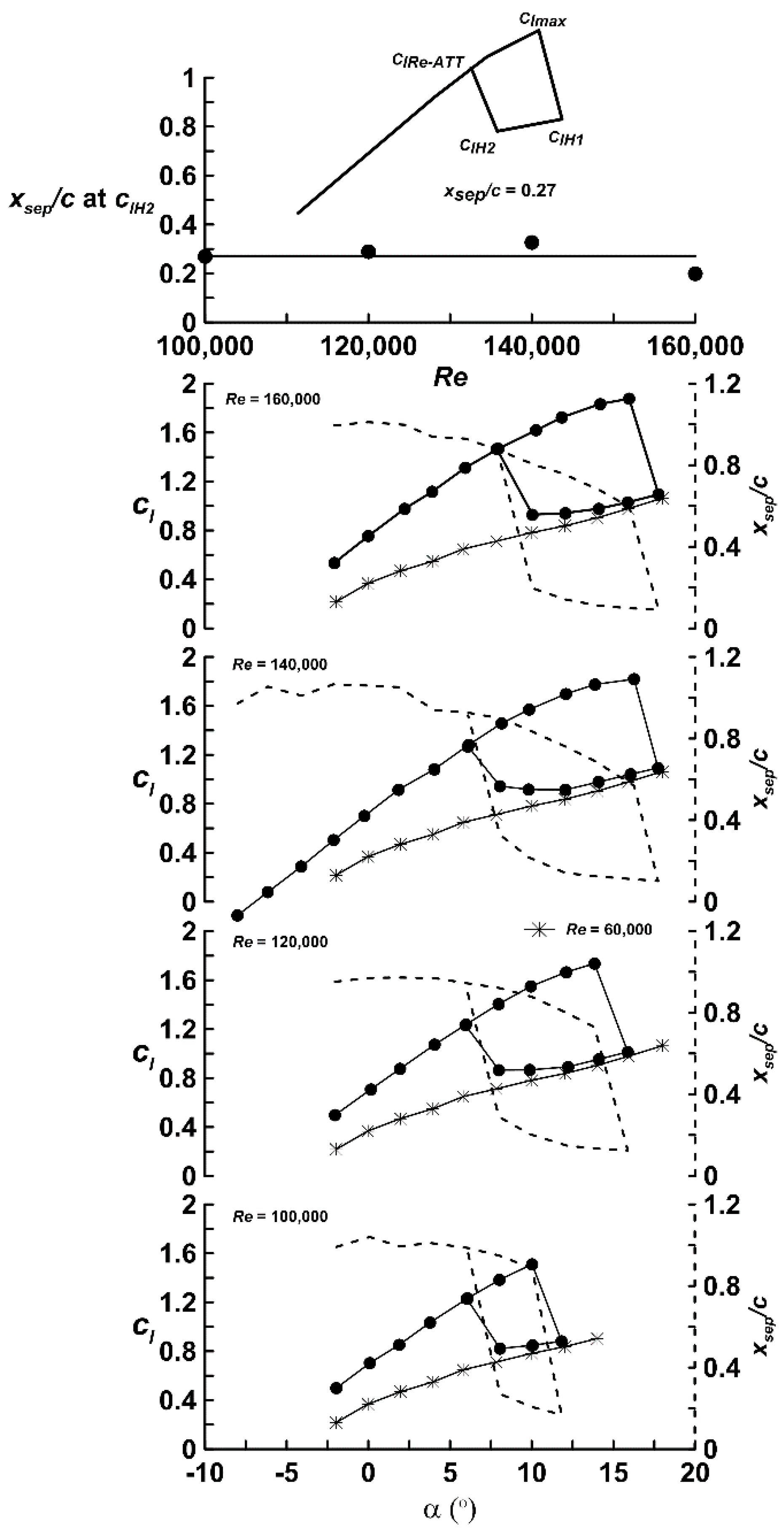
Figure 1 examines the behavior of x_sep/c for E591 airfoil data where a loop was present. The top inset defines nomenclature associated with the lift curve. The plots clearly show a large clockwise hysteresis loop that increases in extent with Reynolds number until Re = 140,000 and then shortens slightly. It may be observed that the lower left most extent of the loop (c_lH2) has a fairly consistent value of x_sep/c for all presented Re; as shown explicitly in the top plot in Figure 1. An average value of x_sep/c = 0.27 is indicated just prior to upper surface flow re-attachment. The dashed lines in Figure 1 show the upper surface boundary layer separation location estimated using Equation (2) and are associated with the right hand vertical axis. The airfoil lift curve slope (c_lα) in Equation (2) is that determined from the most linear extent in the low angle of attack regime. Also included in Figure 1 is data for the E591 at Re = 60,000. As seen, laminar separation without re-attachment is present. Laminar separation without transition and consequently re-attachment precludes hysteresis. The lift coefficient of the lower leg of the loops for all the presented Re cases is seen to coincide (with Re = 60,000), implying that the airfoil is experiencing laminar separation without transition or bubble formation in this regime.

Calculating c_lHyst–Ave/c_lmax for the E591 airfoil showed a strong correlation for all Reynolds number. As seen in Figure 1, both c_lmax and c_lHyst–Ave show Re dependency; c_lmax increases with Re, as does c_lHyst–Ave. However, they do so in proportion such that their ratio is relatively constant. Thus, while these two terms individually show Re sensitivity, their ratio does not for the Re range explored. 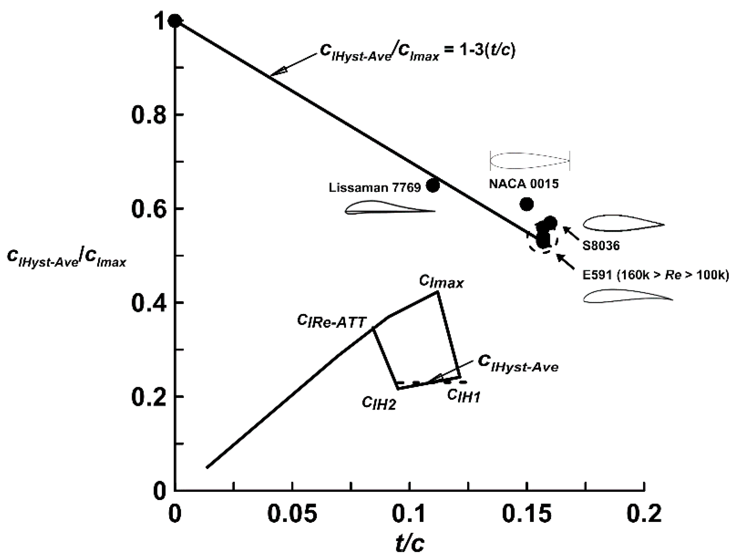Figure 2 examines explicitly c_lHyst–Ave/c_lmax using the aforementioned data. In addition, data for the NACA 0015, S8036 and Lissaman 7769 (t/c = 0.11) [1] are also shown in Figure 2. Examination of airfoil data in Ref. [10] shows little evidence of the existence of hysteresis for airfoils with t/c < 0.09. A thin flat plate does not typically experience hysteresis. This was confirmed through testing of the 0.5% thick flat plate for Re ranging from 40,000 to 160,000. While c_lmax showed a Re dependency for the flat plate, no signs of hysteresis were observed. Thus, a flat plate was included as a bounding case for t/c = 0 with c_lHyst–Ave/c_lmax = 1. A linear variation between c_lHyst–Ave/c_lmax and t/c is indicated in Figure 2 and was curve fitted (using the E591 data and that for the flat plate) to yield:

$$c_{lHyst-Ave} = c_{l\max }\left[1-3\left(\frac{t}{c}\right)\right]$$

(3)

Note that the dependence of c_lHyst–Ave/c_lmax on the airfoil’s leading edge radius as well as its camber’s location and magnitude were also examined without the appearance of any strong correlation. It must be mentioned that for many airfoils, the lift produced in the return loop from c_lH1 to c_lH2 is not constant and may increase or decrease relative to c_lH1 as the airfoil’s angle of attack is reduced, depending on the airfoil geometry. For an engineering estimate however, a constant c_lHyst assumption is acceptable.

Recasting Equation (1) to solve for the incidence just prior to large scale re-attachment, i.e., at the location where x_sep/c = 0.27 gives:

$${\alpha }_{c_{lH2}}={\alpha }_{zl}+\frac{c_{lHyst–Ave}}{c_{l\alpha }{\left[\frac{1+\sqrt{0.27}}{2}\right]}^2}={\alpha }_{zl}+\frac{c_{l\max }\left[1-3\left(\frac{t}{c}\right)\right]}{c_{l\alpha }{\left[\frac{1+\sqrt{0.27}}{2}\right]}^2}={\alpha }_{zl}+\frac{c_{l\max }\left[1-3\left(\frac{t}{c}\right)\right]}{0.577c_{l\alpha }}$$

(4)

To account for loop closure it may be assumed that the slope of lift recovery is the same as that of the lift loss following c_lmax (i.e., the slope from c_lmax to c_lH1) such that:

$${\alpha }_{\text{Re-ATT}}={\alpha }_{c_{lH2}}+\left(\frac{{\alpha }_{c_{l\max }}-{\alpha }_{c_{lH1}}}{c_{l\max }-c_{lH1}}\right)(c_l-c_{lH2})$$

(5)

Equation (5) can be used to construct a line from point α_clH2 until it cuts the initial lift curve yielding the point c_l = c_lRe-ATT. Note that the slope of the re-attachment line is often less severe than that following c_lmax, however, within the spirit of this article, this approximation is consistent.

Hysteresis is extremely sensitive to environmental conditions as noted in References [1,5,11]. Unfortunately, little systematic data of sufficient scope exists that may be used to ascertain an exact dependence of loop behavior on wind tunnel turbulence. Marchman and Sumantran [5] investigated the effect of acoustic and free stream turbulence effects on hysteresis. It was shown that turbulence does not appear to affect the magnitude of the lift loss following stall, but shortens the width of the loop. While the given data is limited, a 2° reduction in angle of attack (for a Wortman FX 63-137 profile, t/c = 0.137)) required for loop closure was recorded for an increase in freestream turbulence intensity from 0.02% to 0.2% (achieved using turbulence strips attached to the screens), indicating earlier boundary layer re-attachment. As a simple approximation, this would imply that:

Δα_Hyst = 11.1[TI(%) − 0.2%]

(6)

Equation (6) should be treated with caution, especially for high values of TI (turbulence intensity), but is used in this article as an initial estimate of turbulence effects on loop closure. An increase in turbulence intensity above 0.2% would be additive to α_clH2, reducing the loop width. The magnitude of Equation (6) should never exceed (α_clH1 – α_clH2). In this case, it may be inferred that the freestream turbulence has eliminated hysteresis.

To implement the correlation the following procedure can be used:

• The experimental (or numerical) lift curve for increasing angle of attack for the airfoil of interest is required, including the region immediately following c_lmax;
• Determine c_lHyst–Ave using Equation (3). Use the experimental value of α at point c_lH1 as indicated in the inset of Figure 1 as the start point of the return loop;
• Determine the length of the return segment of the loop to point c_lH2 using Equation (4);
• If the turbulence intensity of the experimental data differs from 0.2%, add Equation (6) to Equation (4) adjust α_clH2;
• Determine the return segment of the curve from c_lH2 to c_lRe-ATT using Equation (5). Extend the return segment line until it cuts the experimental lift curve at point c_lRe-ATT.

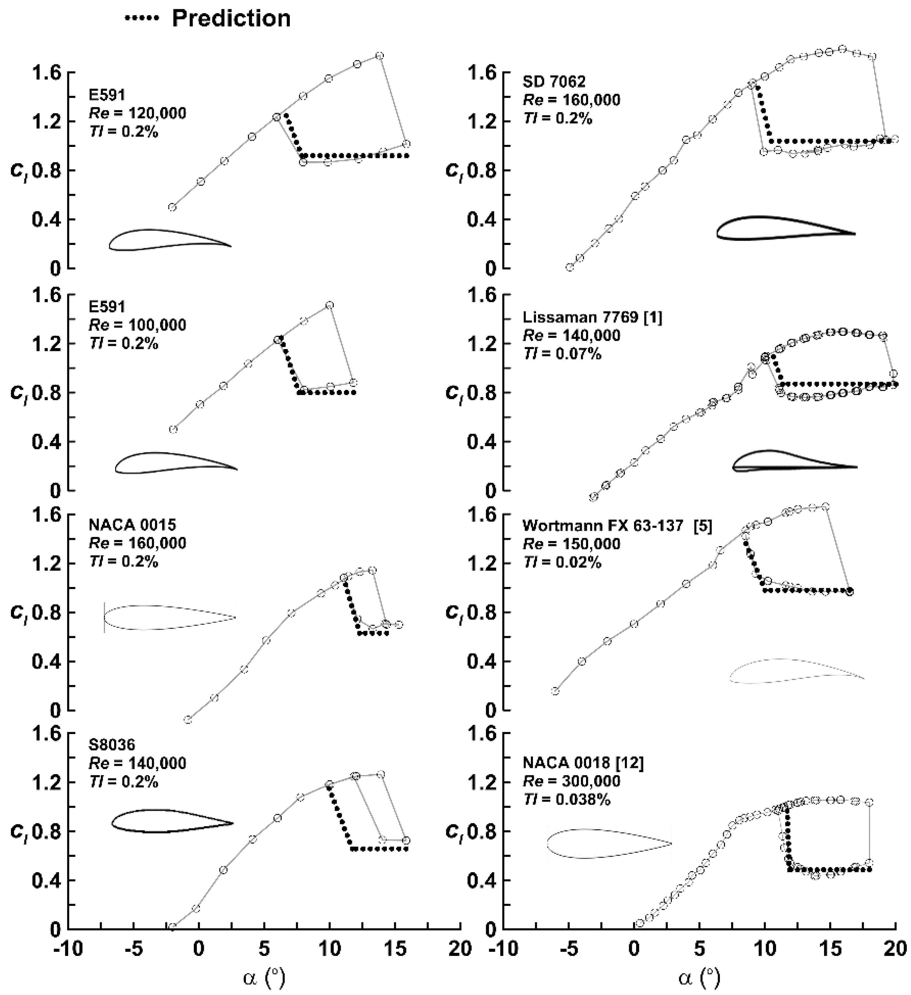
Figure 3 presents comparisons of experiment with prediction. Note that data for the E591 was used to establish the correlations, such that the other six airfoil comparisons (including data from Refs. [1,5,12]) do not represent comparison with data used to formulate the method. As shown, agreement between the correlation and the experimental data is good, especially when considering the complexity of the phenomenon and the simplicity of the method. The c_lH2 error associated with the S8036 airfoil prediction stems from the non-linearity of the lift curve slope in the low α regime. The dependency of hysteresis on airfoil characteristics may be inferred by examination of Equations (3) and (4). Equation (3) shows that the lift coefficient during the return loop is strongly dependent on the airfoil’s thickness, showing a linear dependence; increasing t/c reduces c_lHyst–Ave relative to c_lmax (i.e., greater the t/c, larger the loop). Reynolds number effects on the magnitude of c_l during the return loop (c_lHyst–Ave) are imbedded in the increase in c_lmax commonly associated with an increase in Re (see Figure 1). The α extent of the return loop, quantified in terms of α_clH2 decreases (i.e., an increase in c_lmax decreases the loop width) proportionally to c_lmax for a given airfoil as indicated by examination of Equation (4). An increase in airfoil lift curve slope (through variation of Re) yields an increased loop extent. Airfoils with significant camber (high α_ZL) tend to have larger loops than those with lesser camber. Increasing free stream turbulence causes a reduction in loop angular extent but does not appear to affect the lift coefficient during the return segment (c_lHyst–Ave). Comparisons of the method with data ranging from Re = 100,000 to 300,000 suggest applicability in this range. Caution should be shown for usage outside of this Re range.

Table 1. Comparison between experiment and theory; prediction of α_Re-ATT.

Airfoil	αRe-ATT (°, Experiment)	αRe-ATT (°, [13])	αRe-ATT (°, Present Method)
NACA 0015 (Re = 160,000)	11.1	10.5	11.2
E591 (Re = 100,000)	6.0	8.0	6.1
E591 (Re = 120,000)	6.0	8.0	5.9
S8036 (Re = 140,000)	11.9	9.5	9.8
Lissaman 7769 (Re = 140,000)	10.0	11.3	10.4
Wortmann FX63-137 (Re = 150,000)	8.9	7.5	8.1
SD7062 (Re = 160,000)	8.9	9.0	9.4
NACA 0018 (Re = 300,000)	11.0	12.2	10.9

contains α_Re-ATT estimates from both theory and experiment. Theoretical predictions include the present method and estimates from the method of Rusak and Morris [13]. Agreement between the current method and that of Rusak and Morris is seen to be good.

4. Conclusions

An investigation has been undertaken to establish correlating trends associated with the formation and behavior of clockwise hysteresis loops on airfoils at low Reynolds number. Airfoils ranging from highly cambered to symmetrical were tested. Analysis of the results indicated that the lift attenuation following stall is consistent for many airfoils and is strongly dependent on the airfoil’s thickness. Examination of wind tunnel data using Kirchoff’s zone of constant pressure formulation to estimate the location of leeward surface separation indicated that the location of upper surface separation is close to the ¼ chord just prior to flow re-attachment. Using this information, a simple correlation model was formulated and validated against experimental data. The model provides the average lift coefficient of the lower leg of the loop as well as the loop’s extent in terms of angle of attack required for lift recovery.