
Experimental Aeroelastic Models Design and Wind Tunnel Testing for Correlation with New Theory


Abstract
:
1. Introduction
- (1)
- (2)
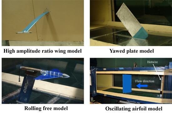
- Wing like plate models, delta wing-store, flapping flag, yawed plate and folding wing. The wing tunnel tests were used to evaluate the von Karman nonlinear plate theory, and a new nonlinear inextensible beam and plate theory and also some high fidelity computation methods. Based on these models several correlation studies for flutter/LCO [6,7,8,9,10,11,12,13,14,15,16] and gust response studies [17,18,19] were performed.
- (3)
- Airfoil section with control surface freeplay. The wing tunnel tests were used to evaluate new approaches for the freeplay nonlinear and gust responses including Duke computational codes using the Peter’s finite state airload aerodynamic theory, harmonic balance method, and the time marching integration based on state space equations [20,21,22,23,24] and the ZAERO code [25] based on the computational fluid dynamic (CFD) theory conducted by ZONA Technology, Inc.
- (4)
- (5)
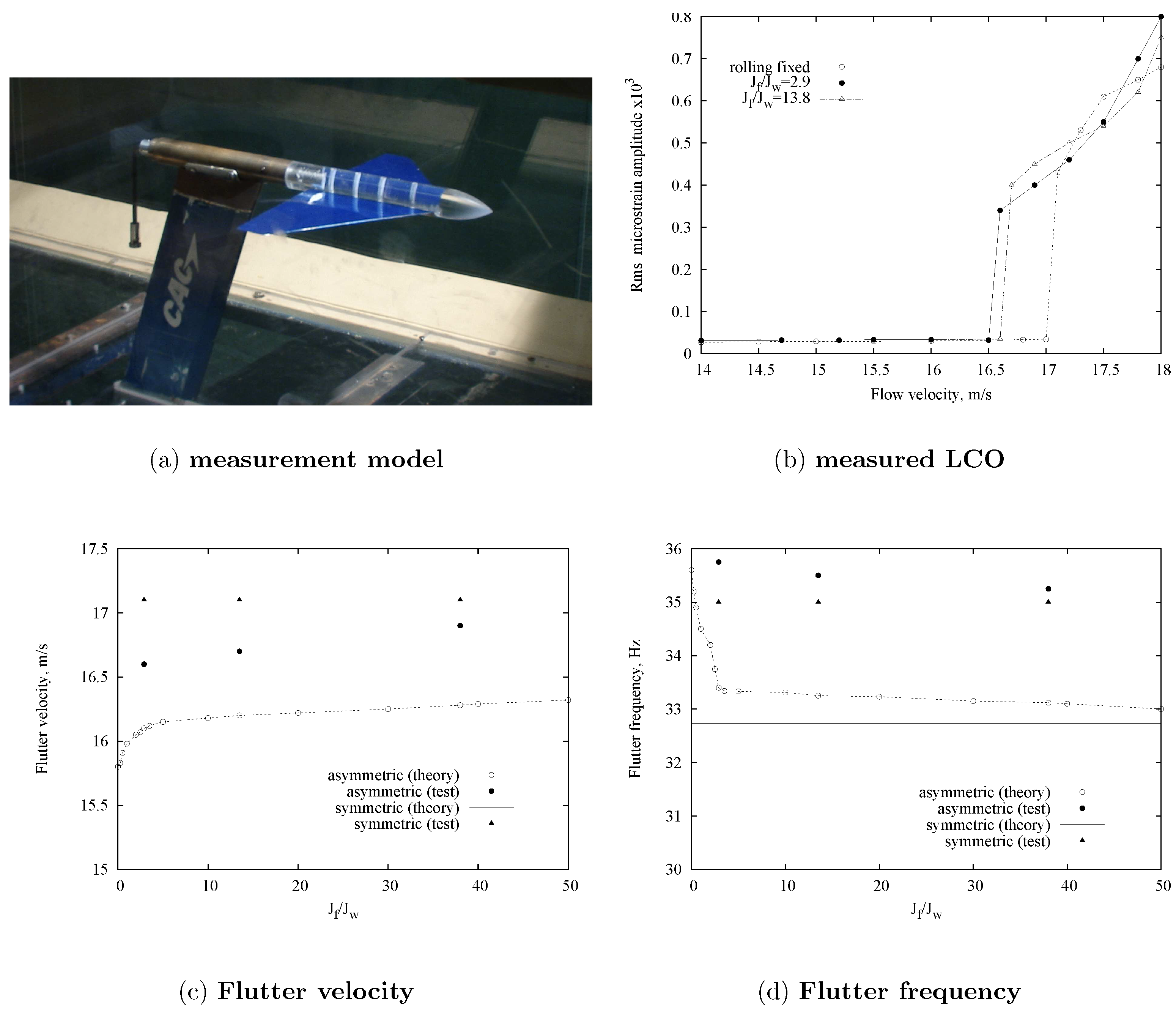
- A free-to-roll fuselage flutter model [28]. From measured wind tunnel data, one evaluates the predicted symmetric and anti-symmetric flutter/LCO theory.
- (6)
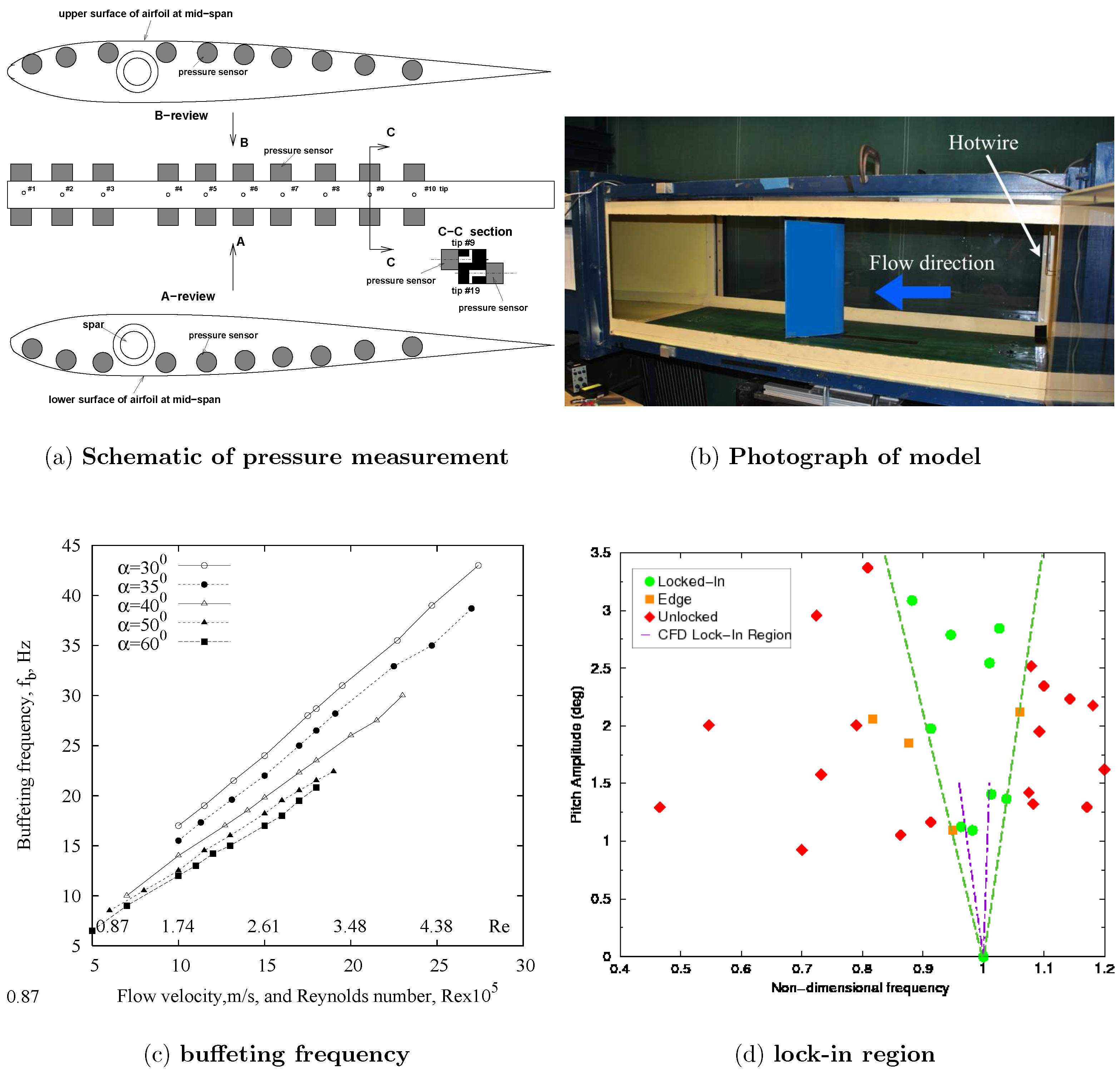
- An experimental oscillating airfoil model at high angles of attack for measuring aerodynamic response. A frequency “Lock-in” phenomenon is found in buffeting flow and compared to the theoretical results [29]. Also, an experimental airfoil model with a portial-span control surface is conducted to measure the flap response of the portial-span induced by the buffeting flow [30].
2. Experimental Models for Measuring Flutter/Limit Cycle Oscillation (LCO) Response to Evaluate a Nonlinear Structural Theory
2.1. High Altitude Long Endurance Models (Nonlinear Beam Structural Theory and ONERA Aerodynamic Model)
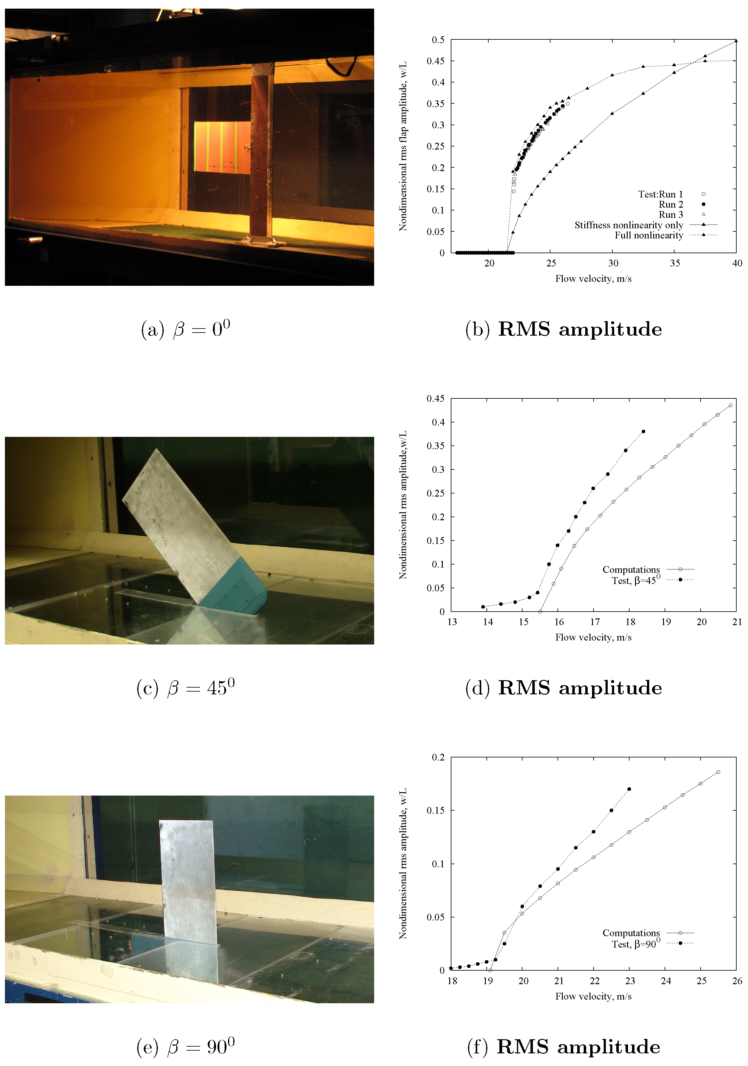
2.2. Flapping Flag and Yawed Plate Models (Nonlinear Inextensible Beam and Plate Theory)
2.3. Free-to Roll Fuselage Flutter Model (Symmetric and Anti-Symmetric Flutter/LCO Theory)
3. Experimental Models for Measuring Flutter/LCO Response to Evaluate Nonlinear Freeplay Theory
3.1. Airfoil Section with Control Surface Freeplay
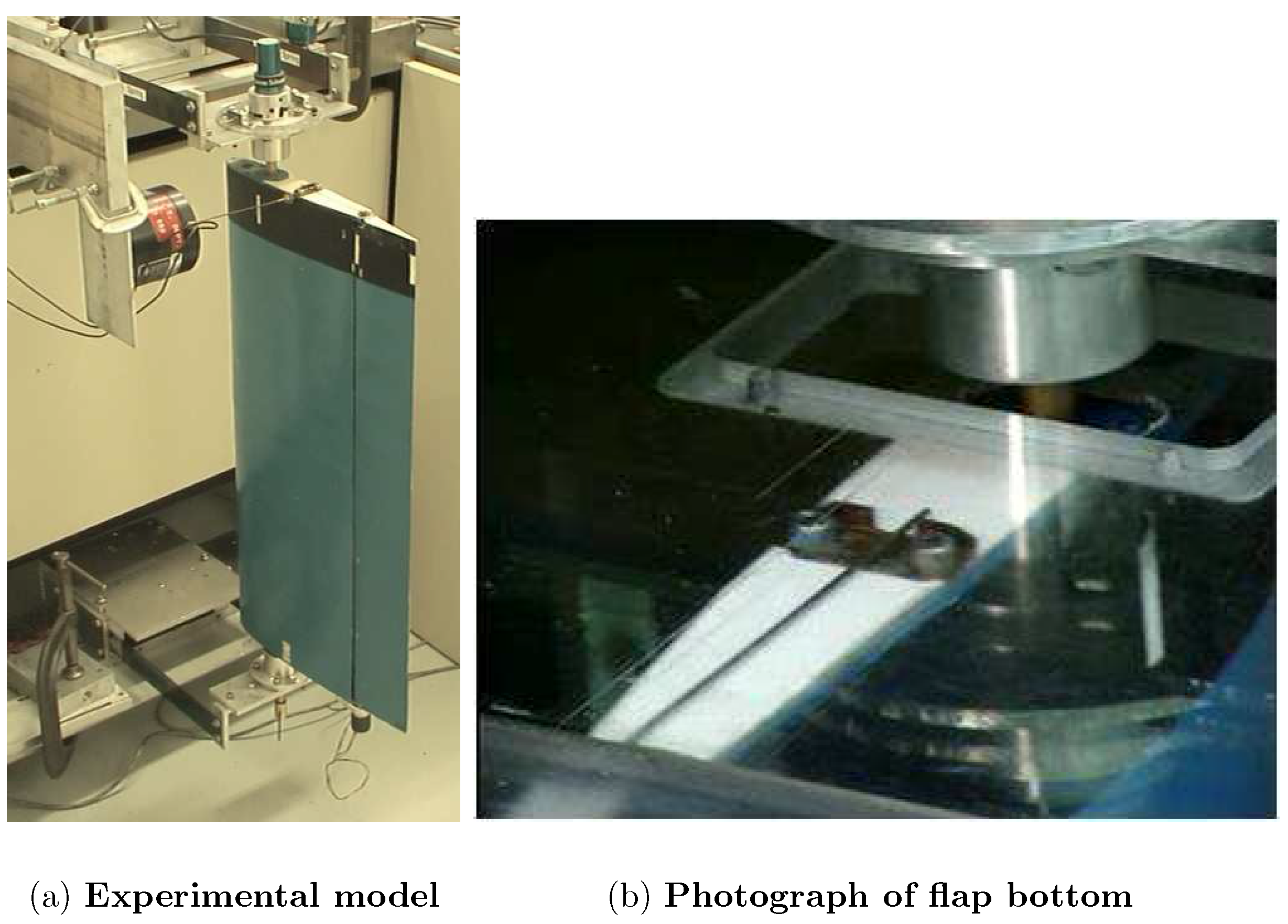
Experimental Model and Measurement System
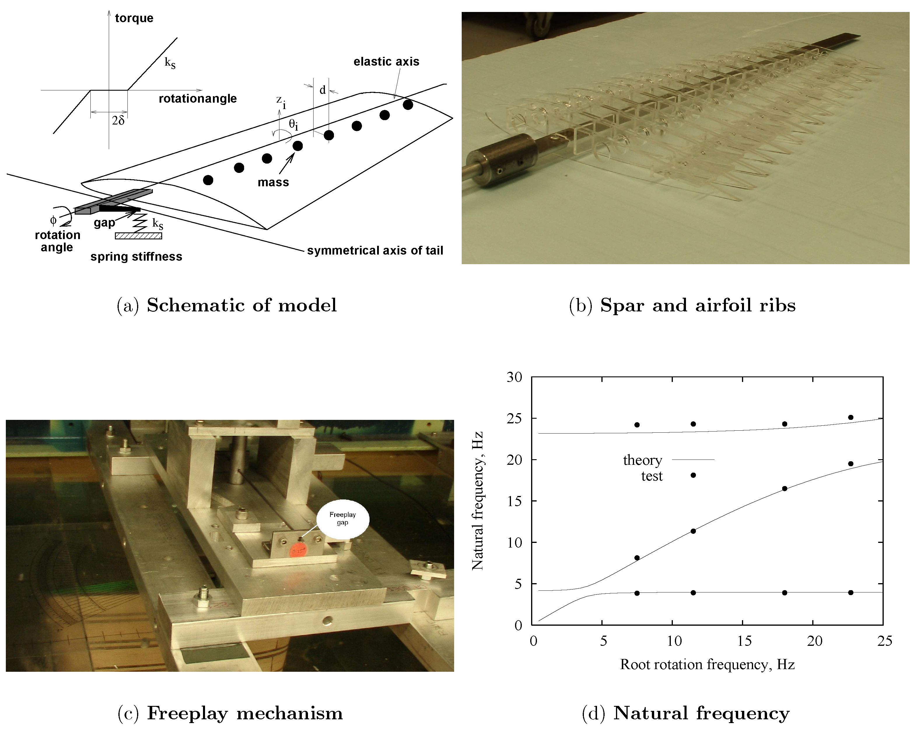
3.2. All-Movable Tail Model with Freeplay
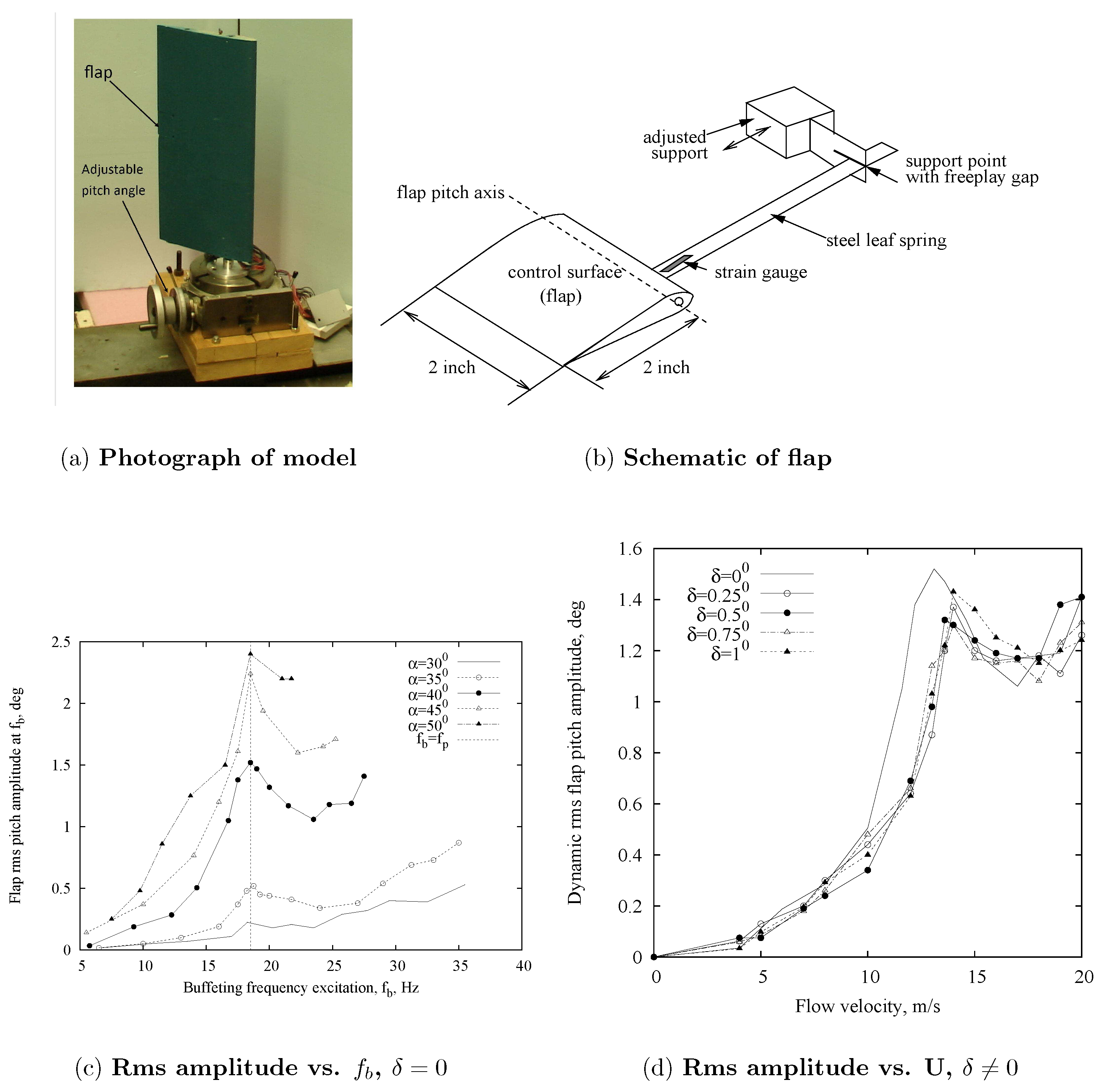
3.2.1. Experimental Model and Measurement System
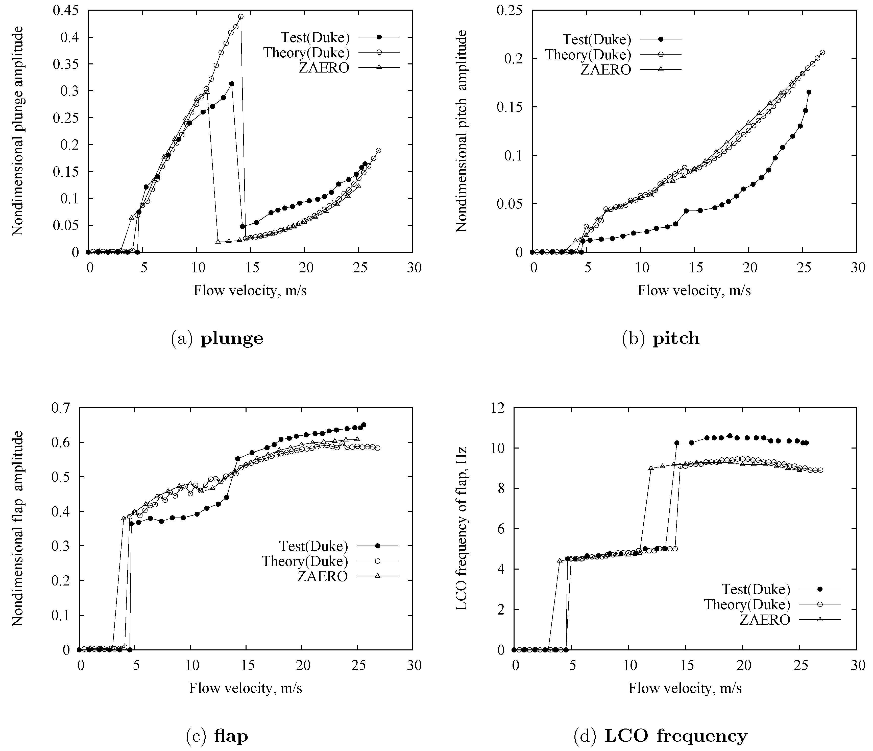
3.2.2. LCO Correlation Study for = 0
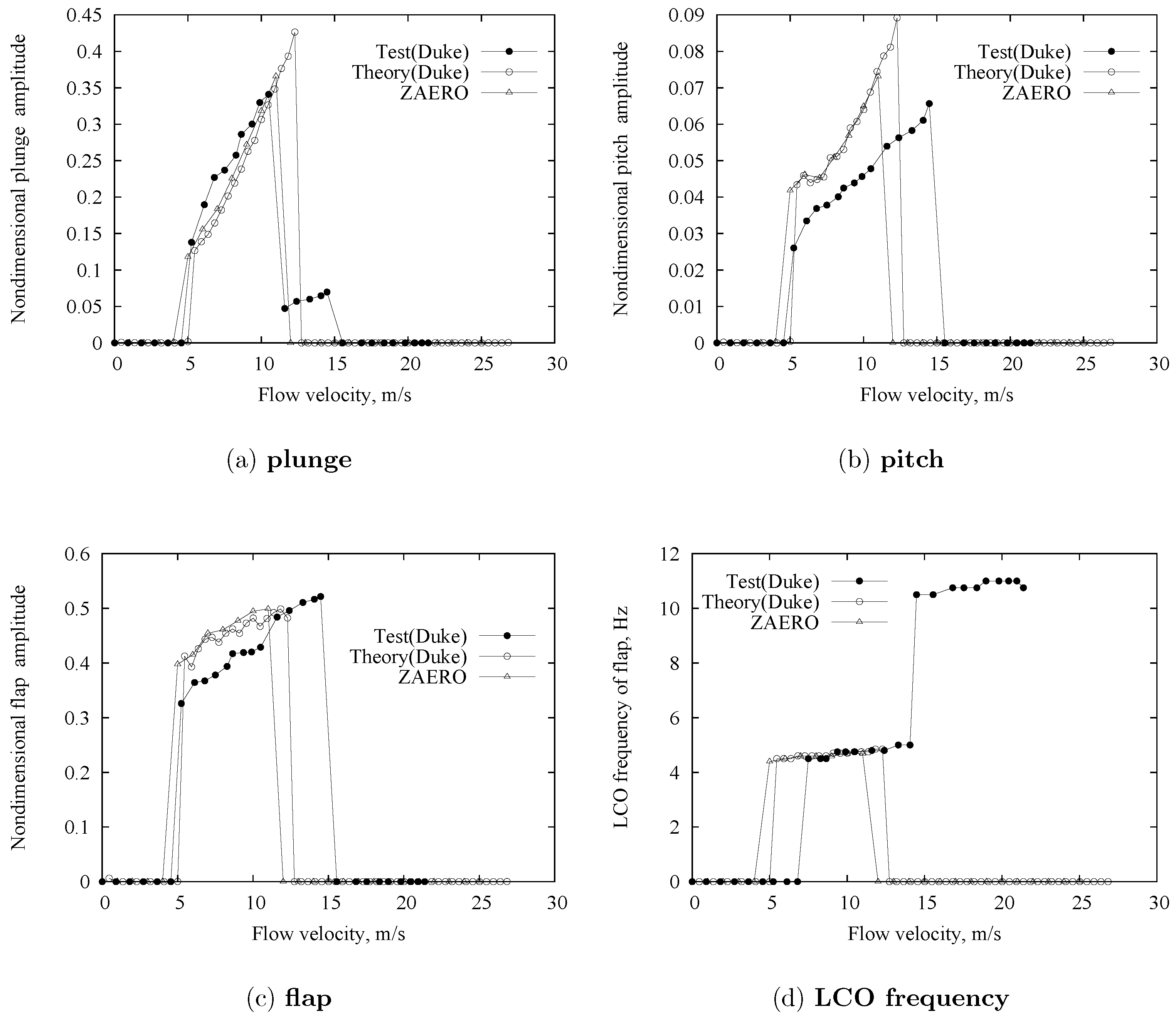
3.2.3. LCO Correlation Study for ≠ 0
4. Experimental Models for Measuring Aerodynamic Response Phenomenon in Buffeting Flow
4.1. An Oscillating Airfoil Section Model in Buffeting Flow
4.1.1. Experimental Model and Measurement System
4.1.2. Correlation Analyses for Frequency Lock-in Region
4.2. An Airfoil with and without Freeplay Control Surface in Buffeting Flow
4.2.1. Experimental Model and Measurement System
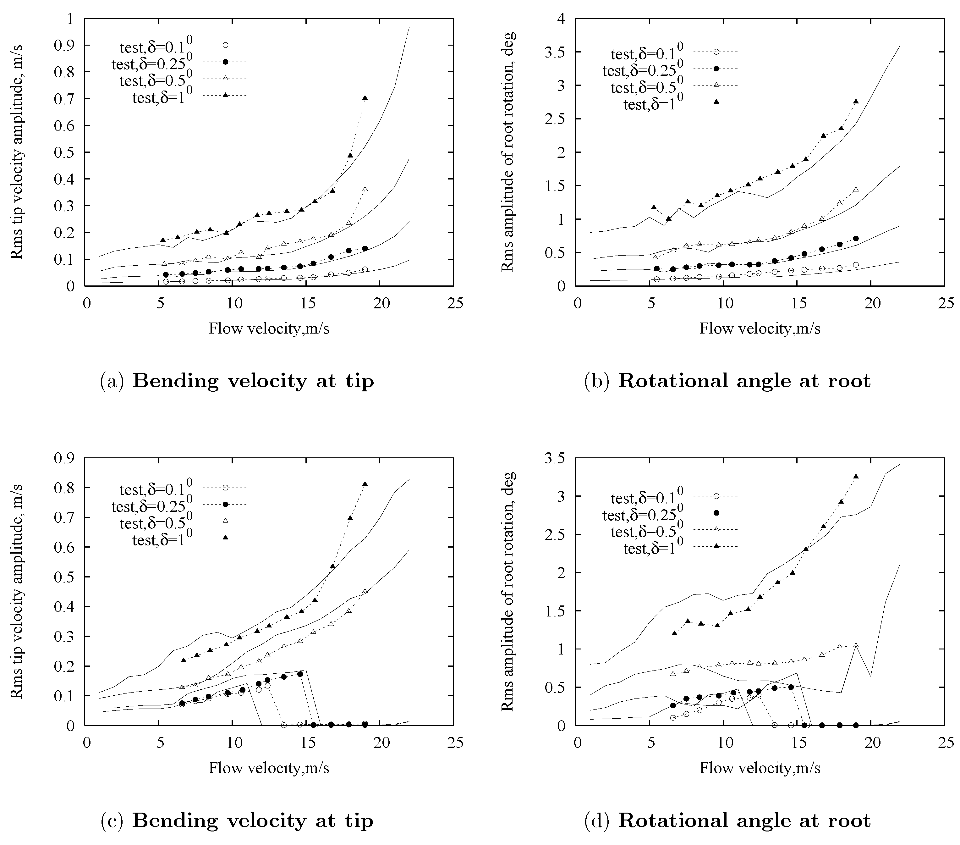
4.2.2. Measured Aeroelastic Response of the Flap Induced by Buffeting Flow
5. Conclusions
Acknowledgments
Author Contributions
Conflicts of Interest
References
- Tang, D.M.; Dowell, E.H. Experimental and Theoretical Study on Aeroelastic Response of High-Aspect Ratio Wings. AIAA J. 2001, 39, 1430–1441. [Google Scholar] [CrossRef]
- Tang, D.M.; Dowell, E.H. Limit Cycle Hysteresis Response for a High-Aspect Ratio Wing Model. J. Aircr. 2002, 39, 885–888. [Google Scholar] [CrossRef]
- Tang, D.M.; Dowell, E.H. Experimental and Theoretical Study of Gust Response for a High-Aspect Ratio Wing. AIAA J. 2002, 40, 419–429. [Google Scholar] [CrossRef]
- Tang, D.M.; Grasch, A.; Dowell, E.H. Gust Response for Flexibly Suspended High-Aspect Ratio Wing. AIAA J. 2010, 48, 2430–2444. [Google Scholar] [CrossRef]
- Tang, D.M.; Dowell, E.H. Flutter/LCO Suppression of High Aspect Ratio Wings. J. R. Aeronaut. Soc. 2009, 113, 409–416. [Google Scholar] [CrossRef]
- Tang, D.M.; Henry, J.K.; Dowell, E.H. Limit Cycle Oscillations of Delta Wing Models in Low Subsonic Flow. AIAA J. 1999, 37, 1355–1362. [Google Scholar] [CrossRef]
- Tang, D.M.; Dowell, E.H. Effects of Angle of Attack on Nonlinear Flutter of a Delta Wing. AIAA J. 2001, 39, 15–21. [Google Scholar] [CrossRef]
- Tang, D.M.; Attar, P. J.; Dowell, E.H. Flutter/LCO Analysis and Experiment for a Wing-Store Model. AIAA J. 2006, 44, 1662–1675. [Google Scholar] [CrossRef]
- Tang, D.M.; Dowell, E.H. Flutter and Limit Cycle Oscillations for a Wing-Store Model with Freeplay. J. Aircr. 2006, 43, 487–503. [Google Scholar] [CrossRef]
- Attar, P.J.; Dowell, E.H.; Tang, D.M. Modeling the LCO of a Delta Wing Model with an External Store Using a High Fidelity Structural Model. In Proceedings of the AIAA SDM Conference, Austin, Texas, 18–21 April 2005.
- Tang, D.M.; Yamamoto, H.; Dowell, E.H. Experimental and Theoretical Study on Limit Cycle Oscillations of Two-Dimensional Panels in Axial Flow. J. Fluids Struct. 2003, 17, 225–242. [Google Scholar] [CrossRef]
- Gibbs, C.; Sethna, A.; Wang, I.; Tang, D.M.; Dowell, E.H. Aeroelastic Stability of a Cantilevered Plate in Yawed Subsonic Flow. J. Fluids Struct. 2014, 49, 450–462. [Google Scholar] [CrossRef]
- Tang, D.M.; Gibbs, C.; Dowell, E.H. Nonlinear Aeroelastic Analysis with Inextensible Plate Theory Including Correlation with Experiment. AIAA J. 2015, 53, 1299–1308. [Google Scholar] [CrossRef]
- Attar, P.J.; Dowell, E.H.; Tang, D.M. A Theoretical and Experimental Investigation of the Effects of a Steady Angle of Attack on the Nonlinear Flutter of a Delta Wing Plate Model. J. Fluids Struct. 2003, 17, 243–259. [Google Scholar] [CrossRef]
- Tang, D.M.; Dowell, E.H. Theoretical and Experimental Aeroelastic Study for Folding Wing Structures. J. Aircr. 2008, 45, 1136–1147. [Google Scholar] [CrossRef]
- Peter, J.A.; Tang, D.M.; Dowell, E.H. Nonlinear Aeroelastic Study for Folding Wing Structures. AIAA J. 2010, 48, 2187–2195. [Google Scholar]
- Tang, D.M.; Henry, J.K.; Dowell, E.H. Nonlinear Aeroelastic Response of a Delta Wing to Periodic Gust. J. Aircr. 2000, 37, 155–164. [Google Scholar] [CrossRef]
- Tang, D.M.; Henry, J.K.; Dowell, E.H. Effects of Steady Angle of Attack on Nonlinear Gust Response of a Delta Wing Model. J. Fluids Struct. 2002, 16, 1093–1110. [Google Scholar] [CrossRef]
- Tang, D.M.; Dowell, E.H. Experimental and Theoretical Study of Gust Response for a Wing-Store Model with Freeplay. J. Sound Vib. 2006, 295, 659–684. [Google Scholar] [CrossRef]
- Conner, M.C.; Tang, D.M.; Dowell, E.H.; Virgin, L.N. Nonlinear Behavior of a Typical Airfoil Section with Control Surface Freeplay: A Numerical and Experimental Study. J. Fluids Struct. 1997, 11, 89–112. [Google Scholar] [CrossRef]
- Tang, D.M.; Dowell, E.H.; Virgin, L.N. Limit Cycle Behavior of an Airfoil with a Control Surface. J. Fluids Struct. 1998, 12, 839–858. [Google Scholar] [CrossRef]
- Tang, D.M.; Kholodar, D.; Dowell, E.H. Nonlinear Aeroelastic Response of a Typical Airfoil Section with Control Surface Freeplay. In Proceedings of the 41st Structures, Structural Dynamics, and Materials Conference and Exhibit, AIAA 2000-1621, Atlanta, GA, USA, 3–6 April 2000.
- Tang, D.M.; Dowell, E.H. Aeroelastic Airfoil with Free Play at Angle of Attack with Gust Excition. AIAA J. 2010, 48, 427–442. [Google Scholar] [CrossRef]
- Tang, D.M.; Gavin, H.P.; Dowell, E.H. Study of Airfoil Gust Response Alleviation Using an Electro-Magnetic Dry Friction Damper–Part 2: Experiment. J. Sound Vib. 2004, 267, 875–897. [Google Scholar] [CrossRef]
- Lee, D.-H.; Chen, P.C.; Tang, D.M.; Dowell, E.H. Nonlinear Gust Response of a Control Surface with Freeplay. In Proceedings of the 51st AIAA/ASME/AHS/ASC Structures, Structural Dynamics and Materials Conference, AIAA 2010-3116, Oriando, FL, USA, 12–15 April 2010.
- Tang, D.M.; Dowell, E.H. Aeroelastic Response Induced by Freeplay: Part II, Theoretical/Experimental Correlation Analysis. AIAA J. 2011, 49, 2543–2554. [Google Scholar] [CrossRef]
- Tang, D.M.; Dowell, E.H. Computational/Experimental Aeroelastic Study For A Horizontal Tail Model with Freeplay. AIAA J. 2013, 51, 341–352. [Google Scholar] [CrossRef]
- Tang, D.M.; Dowell, E.H. Effects of a Free-to-Roll Fuselage On Wing Flutter: Theory and Experiment. AIAA J. 2014, 52, 2625–2632. [Google Scholar] [CrossRef]
- Tang, D.M.; Dowell, E.H. Experimental Aerodynamic Response for an Oscillating Airfoil in Buffeting Flow. AIAA J. 2014, 52, 1170–1179. [Google Scholar] [CrossRef]
- Tang, D.M.; Dowell, E.H. Experimental Aeroelastic Response for a Freeplay Control Surface in Buffeting Flow. AIAA J. 2013, 51, 2852–2861. [Google Scholar] [CrossRef]
- Hodges, D.H.; Dowell, E.H. Nonlinear Equations of Motion for the Elastic Bending and Torsion of Twisted Nonuniform Rotor Blades; Technical Report NASA TN D-7818; NASA: Washington, DC, USA, 1974.
- Tran, C.T.; Petot, D. Semi-Empirical Model for the Dynamic Stall of Airfoils in View to the Application to the Calculation of Responses of a Helicopter Blade in Forward Flight. Vertica 1981, 5, 35–53. [Google Scholar]
- Simmonds, J.G.; Libal, A. Exact equations for the inextensional deformation of cantilevered plates. J. Appl. Mech. 1979, 46, 631–636. [Google Scholar] [CrossRef]
- Simmonds, J.G.; Libal, A. Alternate exact equations for the inextensional deformation of arbitrary, quadrilateral, and triangular plates. J. Appl. Mech. 1979, 46, 895–900. [Google Scholar] [CrossRef]
- Simmonds, J.G. Exact equations for the large inextensional motion of plates. J. Appl. Mech. 1981, 48, 109–112. [Google Scholar] [CrossRef]
- Darmon, P.; Benson, R.G. Numerical Solution to an Inextensible Plate Theory with Experimental Results. J. Appl. Mech. 1986, 53, 886–890. [Google Scholar] [CrossRef]
- Tang, D.M.; Zhao, M.; Dowell, E.H. Inextensible Beam and Plate Theory: Computational Analysis and Comparison with Experiment. J. Appl. Mech. 2014, 81. [Google Scholar] [CrossRef]
- Molyneux, W.G. The Flutter of Swept and Unswept Wing with Fixed-Root Conditions; HM Stationery Office: London, UK, 1950. [Google Scholar]
- Yates, E.C., Jr. AGARD Standard Aeroelastic Configurations for Dynamic Response I—Wing 445.6; NASA-TM-100492; NASA Langley Research Center: Hampton, VA, USA, 1 August 1987.
- Weatin, M.F.; Goes, L.C.; Ramos, R.L.; Silva, R.G. Aeroservoelastic Modeling of a Flexible Wing for Wind Tunnel Flutter Test. In Proceedings of 20th International Congress of Mechanical Engineering (p.9), Gramado, RS, Brasil, 15–20 November 2009.
- Edwards, J.W.; Schuster, D.M.; Spain, C.V.; Keller, D.F.; Moses, R.M. MAVRIC Flutter Model Transonic Limit Cycle Oscillation Test. In Proceeding of the 19th AIAA Applied Aerodynamics Conference, AIAA-2001-1291, Anaheim, CA, USA, 16–19 April 2001.
- Peters, D.A.; Cao, W.M. Finite State Induced Flow Models, Part I: Two-Dimensional Thin Airfoil. J. Aircr. 1995, 32, 313–322. [Google Scholar] [CrossRef]
- Niles, R.H.; Spielberg, I.N. Subsonic Flutter Tests of an Unswept All-Movable Horizontal Tail; WADC TR-54-53, AD 39949; Wright Air Development Center Wright-Patterson AFB: Dayton, OH, USA, March 1954. [Google Scholar]
- Niles, R.H. Subsonic Flutter Model Tests of an All-Movable Stabilizer with 35° Sweepback; WADC Technical Note 55-623, AD 91593; Wright Air Development Center Wright-Patterson AFB: Dayton, OH, USA, November 1955. [Google Scholar]
- Cooley, D.E.; Murphy, J.A. Subsonic Flutter Model Tests of a Low Aspect Ratio Unswept All-Movable Tail; WADC-TR-58-31, AD 142337; Wright Air Development Center Wright-Patterson AFB: Dayton, OH, USA, February 1958. [Google Scholar]
- Raveh, D.E. Numerical Study of an Oscillating Airfoil in Transonic Buffeting Flows. AIAA J. 2009, 47, 505–515. [Google Scholar] [CrossRef]
- Raveh, D.E.; Dowell, E.H. Frequency Lock-in Phenomenon for Oscillating Airfoils in Buffeting Flows. J. Fluids Struct. 2011, 27, 89–104. [Google Scholar] [CrossRef]
- Dowell, E.H.; Hall, K.C.; Thomas, J.P.; Kielb, R.E.; Spiker, M.A.; Denegri, C.M., Jr. A New Solution Method for Unsteady Flows Around Oscillating Bluff Bodies. In IUTAM Symposium on Fluid-Structure Interaction in Ocean Engineering, Proceedings of the IUTAM Symposium, Hamburg, Germany, 23–26 July 2007; Springer: New York, NY, USA; p. 37.
- Chen, J.; Fang, Y.C. Lock-on of Vortex Shedding due to Rotational Oscillations of a Flat Plane in a Uniform Stream. J. Fluid Struct. 1997, 12, 779–798. [Google Scholar] [CrossRef]
- Hall, K.C.; Thomas, J.P.; Clark, W.S. Computation of Unsteady Nonlinear Flows in Cascades Using a Harmonic Balance Technique. AIAA J. 2002, 40, 879–886. [Google Scholar] [CrossRef]
- Besem, F.; Kamrass, J.D.; Thomas, J.P.; Tang, D.M.; Kielb, R.E. Vortex-Induced Vibration and Frequency Lock-in of An Airfoil at High Angles of Attack. J. Fluids Eng. Trans. ASME 2016, 138. [Google Scholar] [CrossRef]


| Wing Properties | |
|---|---|
| Span (L) | 0.4508 m |
| Chord (c) | 0.0508 m |
| Mass per unit length | 0.2351 kg/m |
| Mom. Inertia (50% chord) | 0.2056 × 10 kgm |
| Spanwise elastic axis | 50% chord |
| Center of gravity | 49% chord |
| Flap bending rigidity () | 0.4186 Nm |
| Chordwise bending rigidity () | 0.1844 × 10 Nm |
| Torsional rigidity () | 0.9539 Nm |
| Flap structural modal damping () | 0.02 |
| Chordwise structural modal damping () | 0.025 |
| Torsional structural modal damping () | 0.031 |
| Slender Body Properties | |
| Radius (R) | 0.4762 × 10 m |
| Chord length ( | 0.1406 m |
| Mass (M) | 0.0417 kg |
| Mom. Inertia () | 0.9753 × 10 kgm |
| Mom. Inertia () | 0.3783 × 10 kgm |
| Mom. Inertia () | 0.9753 × 10 kgm |
| E | h | L | C | |
|---|---|---|---|---|
| 2840 kg/m | 70.6 × 10 N/m | 0.381 mm | 275 mm | 151 mm |
| Mode | ANSYS Code | Experiment | Error |
|---|---|---|---|
| Freq (Hz) | Freq (Hz) | (Percent) | |
| 1st Bending | 4.16 | 3.95 | 5.06 |
| 2nd Bending | 25.84 | 24.98 | 3.3 |
| 3rd Bending | 72.12 | 69.91 | 3.06 |
| 4th Bending | 144.06 | 142.37 | 1.1 |
| 1st Twist | 15.91 | 15.13 | 3.45 |
| 2nd Twist | 45.73 | 49.05 | 7.16 |
| Model Parameters: | |
|---|---|
| Chord | 0.254 m |
| Span | 0.52 m |
| Semi-chord (b) | 0.127 |
| Elastic axis (a) w/r/t (b) | −0.5 |
| Hinge line (c) w/r/t (b) | 0.5 |
| Mass Parameters: | |
| Mass of wing | 0.713 kg |
| Mass of aileron | 0.18597 kg |
| Mass/length of wing-aileron | 1.73 kg/m |
| Mass of support blocks | kg |
| Total mass per span, | 3.625 kg/m |
| Inertial Parameters: | |
| (per apn) | 0.0726 kg |
| (per span) | 0.00393 kg |
| (per span) | 0.0185 kgm |
| (per span) | 0.00025 kgm |
| Stiffness Parameters: | |
| (per span) | 46.88 kgm/s |
| (per span) | 2.586 kgm/s |
| (per span) | 2755.4 kg/ms |
| Damping Parameters: | |
| (half-power) | 0.0175 |
| (half-power) | 0.032 |
| (half-power) | 0.0033 |
| Computational | Experimental | % Difference | |
|---|---|---|---|
| (coupled) | 8.32 Hz | 8.45 Hz | 1.6 |
| (coupled) | 17.64 Hz | 17.37 Hz | 1.5 |
| (coupled) | 4.37 Hz | 4.45 Hz | 1.83 |
| (m/s) | 27.3 | 26.5 | 2.9 |
| (Hz) | 6.05 | 6.25 | 3.3 |
| /δ | 0.1 | 0.25 | 0.5 | 1.0 |
|---|---|---|---|---|
| 1 | 17/(15.7) m/s | None | None | None |
| 2 | 12/(13.5) m/s | 16/(14.6) m/s | None | None |
| 4 | 8/(0) m/s | 13/(11) m/s | 16/(14.1) | None |
| 6 | 0/(0) m/s | 10/(0) m/s | 15/(13) | 17/(14.7) |
| 8 | 0/(0) m/s | 0/(0) m/s | 13.5/(0) | 15.5/(12) |
© 2016 by the authors; licensee MDPI, Basel, Switzerland. This article is an open access article distributed under the terms and conditions of the Creative Commons by Attribution (CC-BY) license (http://creativecommons.org/licenses/by/4.0/).
Share and Cite
Tang, D.; Dowell, E.H. Experimental Aeroelastic Models Design and Wind Tunnel Testing for Correlation with New Theory. Aerospace 2016, 3, 12. https://doi.org/10.3390/aerospace3020012
Tang D, Dowell EH. Experimental Aeroelastic Models Design and Wind Tunnel Testing for Correlation with New Theory. Aerospace. 2016; 3(2):12. https://doi.org/10.3390/aerospace3020012
Chicago/Turabian StyleTang, Deman, and Earl H. Dowell. 2016. "Experimental Aeroelastic Models Design and Wind Tunnel Testing for Correlation with New Theory" Aerospace 3, no. 2: 12. https://doi.org/10.3390/aerospace3020012
APA StyleTang, D., & Dowell, E. H. (2016). Experimental Aeroelastic Models Design and Wind Tunnel Testing for Correlation with New Theory. Aerospace, 3(2), 12. https://doi.org/10.3390/aerospace3020012