Enhancing Urban Air Mobility Scheduling Through Declarative Reasoning and Stakeholder Modeling

Abstract

The goal of this paper is to optimize mission schedules for vertical airports (vertiports in short) to satisfy the different needs of stakeholders. We model the problem as a resource-constrained project scheduling problem (RCPSP) to obtain the best resource allocation and schedule. As a new approach to solving the RCPSP, we propose answer set programming (ASP). This is in contrast to the existing research using MILP as a solution to the RCPSP. Our approach can take complex scheduling restrictions and stakeholder-specific requirements. In addition, we formalize and include stakeholder needs using a knowledge representation and reasoning framework. Our experiments show that the proposed method can generate practical schedules that reflect what stakeholders actually need. In particular, we show that our approach can compute optimal schedules more efficiently and flexibly than previous approaches. We believe that this approach is suitable for the dynamic and complex environments of vertiports.

1. Introduction

UAM Air Traffic Management (UATM) safely and efficiently coordinates electric vertical takeoff and landing (eVTOL) vehicles into densely populated urban airspace, contributing to next-generation transportation networks. UATM differs from the traditional methods of air traffic control. It specifically has to coordinate shared urban airspace while satisfying the needs of low-altitude operations with high frequencies and strict safety regulations and dealing with unpredictable weather [1,2]. The recent research suggests that developing frameworks for unbiased scheduling and resource allocation is necessary, and the frameworks help to reduce traffic congestion and ensure access to airspace resources [3,4]. Vertiport-centric scheduling—the focus of this work—serves as an important element of UATM, bridging aerial vehicle routing and ground infrastructure management to sustain system-wide efficiency as UAM operations expand.

Urban air mobility (UAM) facilitates rapid and low-emission aerial journeys through the utilization of eVTOL vehicles, transforming urban transportation. Vertiports, within UATM systems, are multifunctional hubs that can handle vehicle arrivals, departures, charging, passenger transfers, etc. [5]. Efficient scheduling at these hubs can reduce congestion, ensure safety, and meet the stakeholders’ diverse demands. These demands include ones from operators and passengers. However, the dynamic and resource-constrained nature that vertiports have—limited landing pads, charging stations, and airspace corridors—presents substantial challenges while we generate feasible and optimal schedules [6,7].

Traditionally, scheduling has depended on the approaches that solve the resource-constrained project scheduling problem (RCPSP), a well-established framework for optimizing tasks under resource limitations [8]. Along this line, mixed-integer linear programming (MILP) formulations of RCPSP have been widely studied [9,10]. However, these methods face unavoidable scalability issues for large UAM scenarios [11]. In addition, the existing scheduling approaches that solve RCPSPs are incapable of addressing stakeholder-specific requirements, such as flexible delay tolerances or over-assignable resources, which are necessary for practical UAM operations. These limitations inspire alternative paradigms to be explored, such as a declarative programming approach like answer set programming (ASP) [12,13,14]. ASP is effective for complicated combinatorial problems but remains unnoticeable in this specific scheduling context [15].

Based on our earlier work on the dynamic properties of UATM systems, we investigate ASP for vertiport scheduling [16,17,18,19]. We particularly used knowledge representation and reasoning techniques within ASP in order to handle detours or temporary vertiport unavailability. This paper expands on the previous research to the distinct problem domain of proactive vertiport resource scheduling. Specifically, we here focus on accommodating diverse stakeholder needs within the scheduling framework.

This paper addresses these gaps with three key contributions. First, we propose a novel ASP-based formulation for RCPSP and compare it against a MILP baseline. As far as we can tell, applying ASP to RCPSP has not been widely explored, and this work takes a step in that ASP outperforms MILP in scalability for large-scale UAM scheduling. Second, we extend RCPSP to incorporate stakeholder-driven scheduling requirements, including (1) strict on-time service guarantees, (2) over-assignable resources (e.g., shared charging stations), and (3) flexibly bounded execution delays for specific stakeholders. Third, we suggest two algorithmic procedures to calculate schedules that meet both RCPSP constraints and stakeholder needs. Afterwards, we provide extensive experimental confirmation of their effectiveness.

The remainder of this paper is structured as follows: Section 2 reviews the related work on RCPSP and UAM scheduling. Section 3 outlines preliminaries, while Section 4 formalizes the problem. Section 5 details our ASP formulations and stakeholder-considered algorithms. Section 6 and Section 7 present experimental results and conclusions, respectively.

2. Related Work

2.1. UAM Scheduling: Challenges and Domain-Specific Approaches

The UAM case study by [20] argues that for the UAM to be advanced, it requires the utilization of data-driven demand, vertiport locations, improved vertiport operations modeling, and aircraft trajectories. In addition, by integrating with advanced scheduling algorithms, its operations can be optimized, resulting in greater throughput and reduced wait times [21].

UAM operations are challenged to be introduced and scaled up by airspace restrictions [22], the workload of air traffic controllers [23], the integration of conventional and UAM flight operations [24], and the absence of robust airspace management strategies [25].

Various stakeholders, including airlines and regulatory bodies, are involved in UAM operations, and their demands require careful management. The authors in [26] pointed out that UAM vehicles should follow established air traffic regulations while communicating with Air Traffic Control (ATC) and interacting within controlled airspace. By adapting from the collaborative decision-making (CDM) technique, the framework [27] shows operations are efficiently maintained. In addition, research from [28,29] addresses that satisfying stakeholders’ needs will become much more important as UAM operations grow.

Recent studies show the challenges to the seamless integration of UAM in the existing urban transportation system [30]. Along this line, the works from [31,32,33] suggest an adaptive (on-demand) operational framework. The research in [34,35] introduces realistic UAM scheduling between heterogeneous small aircraft (including UAM fleets), suggesting a performance-based, multi-resolution model and a robust charging network. The research from [36] proposes strict safety protocols. As such, the dynamic nature of urban mobility presents both opportunities and challenges.

2.2. Resource-Constrained Scheduling: MILP and Heuristics

2.2.1. RCPSP and MILP Formulations

The resource-constrained project scheduling problem (RCPSP) is one of the major problems in operations research, requiring jobs in a project to be scheduled under resource constraints, with mixed-integer linear programming formulations being the major approach. The authors in [10] introduced a new model that accounts for both resource consumption and production, while their previous work in [37] suggested three established MILP models. The authors in [38] discussed ways in which automatic MILP reformulations and cutting plane techniques can optimize non-preemptive RCPSP solutions.

2.2.2. Heuristic and Metaheuristic Approaches

In addition to the MILP, alternative approaches have emerged, such as quantum annealing techniques [39], metaheuristic strategies [40], robust searching methodologies [41], and genetic algorithms [42]. These researchers explore RCPSP by integrating traditional MILP formulations with modern computational techniques and algorithmic strategies in order to optimize project scheduling under resource constraints.

Researchers have used many heuristic and metaheuristic algorithms, often deviating from the methods of linear programming (LP) and mixed integer linear programming (MILP). The author in [43] proposed a genetic algorithm specifically designed for project scheduling under resource constraints, showing its applicability to real-world scheduling challenges. The research in [44] introduced a hybrid approach that integrates genetic algorithms with local search to improve the solution quality of the RCPSP. Their work, particularly, was to improve both precision and computational efficiency.

The author in [45] suggested a differential evolution (DE) approach that utilizes constrained resources. The authors in [46] suggested the hybridization of multiple algorithms, such as particle swarm optimization (PSO) with differential evolution.

The authors of [47] suggested forward–backward improvement strategies for a GA to meet the RCPSP’s complicated needs, and the authors of [48] suggested a combined hybrid metaheuristic from a scatter search and from electromagnetism theory. The approach to decentralized, resource-constrained, multi-project scheduling from [49] shows how flexible resource scheduling methods are when used with optimizing a schedule for a multi-agent system.

2.3. Declarative Approaches: Answer Set Programming (ASP) in Scheduling

A few researchers have shown the possibility to solve complex scheduling problems in ASP. The authors in [50] suggest a way to break down complicated problems into manageable time windows. This would allow operations to be optimized while still following the order of operations. The work in [51] extends this to multi-resource partial-order flexible job-shop scheduling (MPF-JSS) scenarios using difference logic within the ASP framework. ASP is also adaptable in diverse scheduling contexts. In particular, the author in [52] suggests a hybrid scheduling environment. In addition, the work in [53] exemplifies resource-constrained scheduling.

Even though the research above introduced various scheduling problems, none of them stated RCPSP in the ASP formula.

2.4. Stakeholder-Centric Scheduling

The traditional techniques of RCPSP frequently lack adequate mechanisms to satisfy the changing needs of different stakeholders [54,55]. The works in [56,57,58] stick to resource restrictions, minimizing the makespan but not considering the distinctive demands of different stakeholders. In this respect, the authors in [59] proposed flexible structures in order to accommodate resource constraints. However, their work still did not capture the broader stakeholder context. In addition, in order to adapt to changing situations and requirements, the works from [60,61] suggested middle-ground solutions that apply fuzzy logic and heuristics. However, their works lacked systematic approaches to satisfy the varied demands from stakeholders.

Formalizing the requirements from different stakeholders to executable constraints can be inspired by particularly complex, multi-agent systems. The foundational work by [62] demonstrates how timed partial order specifications can enforce temporal and precedence rules, which are adaptable to UAM’s strict on-time guarantees and delay tolerances. This can also be complemented by multi-agent negotiation in resource allocation, such as distributed scheduling protocols [63,64,65], agent communication and coalition [49,66,67], and auction-based methods [68].

3. Preliminaries

3.1. Scenario I: Vertiport Operations as an RCPSP

In the context of vertiport scheduling, jobs represent distinct operational activities such as an electric vertical takeoff and landing vehicle’s arrival, landing, passenger disembarkation, battery charging, passenger embarkation, pre-flight checks, and departure. Each of these activities has an estimated processing time. The resources correspond to limited vertiport assets like landing pads, charging stations, parking stands, and available airspace slots for approach and departure. Each activity requires a certain unit of a specific resource, and these resources have finite capacities. Precedence relations define the necessary sequence of operations; for example, landing must precede charging, and charging must precede the next departure for the same vehicle.

Several typical job sequences can illustrate these operations and their inherent precedences:

• Full Turnaround Sequence: Arrival → Landing → Passenger Disembarkation → Battery Charging → Passenger Embarkation → Pre-flight Checks → Departure. This is a sequence of the general operations that a vehicle drops off passengers, proceeds to required maintenance (like charging), boards new passengers, and then departs. Resources like landing pads, gates or stands, and charging stations are utilized sequentially.
• Quick Drop-off Sequence: Arrival → Landing → Passenger Disembarkation → (Minimal Checks or Preparation) → Departure. This might be used for repositioning flights or short hops where extensive ground services like charging are not immediately required.
• Cargo Operations Sequence: Arrival → Landing → Cargo Unloading → Cargo Loading → Pre-flight Checks → Departure. This is for transporting cargo. Instead of passenger-related jobs, it handles cargo-related jobs.
• Charging-Focused Sequence: Arrival → Landing → Battery Charging → Pre-flight Checks → Departure. This sequence is only for eVTOL to visit the vertiport for charging without handling passengers or cargo.

3.2. RCPSP

The resource-constrained project scheduling problem (RCPSP) is a combinatorial optimization problem where we have to find a feasible plan for a group of n jobs while taking into account limitations on resources and order of priority. Each job has a processing time, a list of jobs that come after it, and a set of resources that it needs. Even though resources may be limited, they can be used again and again. Due to the rules of order, no job can start before all of its predecessors are completed. The jobs must be scheduled without interruption, meaning that once they begin, they cannot be stopped.

The RCPSP accepts the following input:

• J: a set of jobs $\{j\in \mathbb{N}|1\le j\le n\}$,
• R: a set of resources,
• S: a list of the order in which the tasks $(i,j)$ in the jobs will be executed,
• T represents the planning horizon, which is a list of potential completion time steps for jobs,
• $p_j$: the time required to complete job j,
• The formula $u(j,r)$ represents the required unit of resource r to complete job j, and
• $C_r$: the capacity of resource r.

In addition, the job set J contains two dummy jobs, $\{0,n+1\}$, that indicate the beginning and the end of scheduling. The dummies require no resources and have zero processing time.

The following is a binary formulation adapted from [69]. Decision variables $x_{(j,t)}$ are represented as follows:

$$x_{(j,t)}:=\left\{\begin{array}{cc}1\hfill & \mathrm{if}\mathrm{job}j\mathrm{is}\mathrm{assigned}\mathrm{to}\mathrm{begin}\mathrm{at}\mathrm{time}t\hfill \\ 0\hfill & \mathrm{otherwise}\hfill \end{array}\right.$$

(1)

Every job should be assigned at one time following its precedence order and resource restrictions. The entire model is as follows:

$$\begin{array}{ccc}\mathrm{Minimize}\hfill & \hfill & \hfill \sum _{t\in T}t·x_{(n+1,t)}\end{array}$$

(2)

$$\begin{array}{cccccc}\mathrm{Subject}\mathrm{to}\hfill & \hfill \hfill & \hfill \sum _{t\in T}{x}_{(j,t)}& =1\hfill & \hfill & \forall j\in J\hfill \end{array}$$

(3)

$$\begin{array}{cccc}\hfill & \hfill & \hfill \sum _{j\in J}\sum _{t_2=max(0,t-p_j+1)}^t{u}_{(j,r)}·x_{(j,t_2)}\le c_r& \forall t\in T,r\in R\hfill \end{array}$$

(4)

$$\begin{array}{ccccc}\hfill & \hfill & \hfill \sum _{t\in T}t·x_{(s,t)}-\sum _{t\in T}t·x_{(j,t)}\ge p_j& \hfill & \forall (j,s)\in S\hfill \end{array}$$

(5)

$$\begin{array}{ccccc}\hfill & \hfill & \hfill x_{(j,t)}\in \{0,1\}& \hfill & \forall j\in J,t\in T\hfill \end{array}$$

(6)

Below, from Equations (7)–(12), we provide ASP formulations to solve the same problem in a different approach converting from the one in Equations (2)–(6). Figure 1 shows two different resource assignments of the instance in

Table 1. This is a table to represent the instance shown in Figure 1.

Job	Duration	Resources Required			Successors
		Resource 0	Resource 1	Resource 2
1	5			3
2	2	1			1
3	1			2	2
4	5	3	1		2
5	2	3	1		3
6	4			1
7	2			3
8	5	1	3
9	5		1		6, 7
10	4			1	9

. Both are valid, as we can see from the resource graphs shown in side by side.

$$\begin{array}{cc}\hfill \mathtt{1}\{\mathtt{start}(\mathtt{A},\mathtt{I}):\mathtt{step}(\mathtt{I})\}\mathtt{1}\leftarrow & \mathtt{task}(\mathtt{A}).\hfill \\ \hfill \leftarrow & \mathtt{psrel}(\mathtt{P},\mathtt{S}),\mathtt{dur}(\mathtt{P},\mathtt{D}\mathtt{1}),\mathtt{start}(\mathtt{P},\mathtt{I}\mathtt{1}),\mathtt{start}(\mathtt{S},\mathtt{I}\mathtt{2}),\hfill \end{array}$$

(7)

$$\begin{array}{cc}\hfill & \mathtt{I}\mathtt{2}<\mathtt{I}\mathtt{2}+\mathtt{D}\mathtt{1}.\hfill \\ \hfill \mathtt{assigned}\_\mathtt{res}(\mathtt{TS},\mathtt{A},\mathtt{R},\mathtt{AM})\leftarrow & \mathtt{step}(\mathtt{TS}),\mathtt{task}(\mathtt{A}),\mathtt{rsreq}(\mathtt{A},\mathtt{R},\mathtt{AM}),\mathtt{dur}(\mathtt{A},\mathtt{AD}),\hfill \end{array}$$

(8)

$$\begin{array}{cc}\hfill & \mathtt{start}(\mathtt{A},\mathtt{TS}\mathtt{1}),\mathtt{TS}\le \mathtt{TS}<\mathtt{TS}\mathtt{1}+\mathtt{AD}.\hfill \\ \hfill \mathtt{sum}\_\mathtt{assigned}\_\mathtt{res}(\mathtt{TS},\mathtt{R},\mathtt{AM})\leftarrow & \mathtt{step}(\mathtt{TS}),\mathtt{limit}(\mathtt{R},\_),\hfill \end{array}$$

(9)

$$\begin{array}{cc}\hfill & \mathtt{AM}=\#\mathtt{sum}\{\mathtt{AM}\mathtt{1},\mathtt{A}:\mathtt{assigned}\_\mathtt{res}(\mathtt{TS},\mathtt{A},\mathtt{R},\mathtt{AM}\mathtt{1})\}.\hfill \\ \hfill \leftarrow & \mathtt{sum}\_\mathtt{assigned}\_\mathtt{res}(\mathtt{TS},\mathtt{R},\mathtt{AM}),\mathtt{step}(\mathtt{TS}),\mathtt{limit}(\mathtt{R},\mathtt{L}),\hfill \end{array}$$

(10)

$$\begin{array}{cc}\hfill & \mathtt{AM}>\mathtt{L}.\hfill \\ \hfill \mathtt{estart}(\mathtt{I})\leftarrow & \mathtt{start}(\mathtt{A},\mathtt{I}),\mathtt{etask}(\mathtt{A}).\hfill \end{array}$$

(11)

$$\begin{array}{c}\#\mathtt{minimize}\{\mathtt{I}:\mathtt{estart}(\mathtt{I})\}.\hfill \end{array}$$

(12)

For clarity, the core predicates used in Equations (7)–(12) are defined as follows:

• task(A) signifies that A is a task to be scheduled.
• step(I) denotes that I is a discrete time step within the planning horizon.
• The predicate start(A,I) means task A is assigned to begin at time step I.
• dur(A,D) indicates that task A has a processing duration of D time steps.
• Resource requirements are specified by rsreq(A,R,AM), meaning task A requires AM units of resource R.
• The predicate assigned_res(TS,A,R,AM1) is used to track that AM1 units of resource R are assigned to task A at time step TS.
• sum_assigned_res(TS,R,AM) is to calculate the total amount AM of resource R to be assigned at time step TS. This includes all active tasks at this time step.
• limit(R,L) specifies that resource R has a maximum capacity of L units.
• psrel(P,S) is a precedence relation. It means that task P must complete before task S starts.
• Finally, etask(A) identifies A as an end task (specifically, the tail dummy task in this context) whose start time is part of the objective function.

In addition, detailed explanations for some Equations are as follows:

• Equation (8) ensures that every task A is assigned exactly one start time I from the available time steps. The construct 1 {…} 1 is an ASP choice rule, guaranteeing one successful assignment.
• Equation (10) calculates the total resource usage. For a given time step TS and resource R, the component of the rule sums (#sum) all amounts AM1 of that resource assigned to any task A (via assigned_res(TS,A,R,AM1)). The result is unified with AM.
• Equation (12) is the objective function. It instructs the ASP solver to find a schedule that minimizes the value I, where I is the start time of the tail dummy task (identified by estart(I), which is derived from start(A,I), etask(A)). Hence, minimizing the start time of this final dummy task effectively minimizes the overall project makespan.

We remark on the mathematical distinction between MILP and ASP formulations. Unlike MILP, which uses algebraic equations and inequalities, ASP is a declarative programming paradigm. ASP is based on logic programming and stable model semantics. A program in ASP consists of logical rules, and its solutions (answer sets) are the interpretations that satisfy these logical rules. Thus, Equations (7)–(12) are a logical specification of RCPSP constraints, which are different from a direct algebraic representation.

Table 2. Formula Map between MILP and ASP.

Function	MILP	ASP	Description
Objective	Equation (2)	Equation (12)	It minimizes the start time of the tail dummy.
Constraints	Equations (3) and (6)	Equation (7)	Each task should be assigned only once.
	Equation (4)	Equations (9)–(11)	The required resources for each task should be allocated for the duration from its beginning, and the sum of all allocated resources at every time step should not exceed the limit.
	Equation (5)	Equation (8)	Every pair of tasks in the precedence relationship should follow the order.

shows a comparison of the formulas between MILP and ASP.

3.3. Multiple Schedules

We need to address multiple schedules to extend the model to cover individual requirements.

Here, we define a job tree, $\mathcal{J}$, that connects a set of jobs in an execution order.

A schedule can have more than one job tree, $\mathcal{J}$. Therefore, we call a schedule a job forest, $\mathcal{F}$. When we compute a schedule, we add two dummy jobs: one, called a head dummy, at the beginning, and another, called a tail dummy, at the end. Then we connect each head job in ${\mathcal{J}}_i$ to the head dummy and each tail job in ${\mathcal{J}}_i$ to the tail dummy.

Multiple schedules can be specified by ${\mathcal{F}}_i$. If ${\mathcal{F}}_1$ and ${\mathcal{F}}_2$ exist, they are independent of each other. ${\mathcal{F}}_1$ executes its operations first, followed by ${\mathcal{F}}_2$, not simultaneously.

For example, Figure 1 has one schedule ${\mathcal{F}}_1$, two dummies (0 for the head and 11 for the tail), and three job trees. ${\mathcal{J}}_1$ is $\{4,5,3,2,1\}$, ${\mathcal{J}}_2$ is $\{8,6,7\}$, and ${\mathcal{J}}_3$ is $\{10,9\}$.

3.4. Requirements

There are stakeholders. Each of them has its own goal for the Vertiport operation. The goal is to deliver passengers and/or cargo from point A to point B, taking into account connected transportation services. In addition, they need to specify their operational requirements based on their business needs.

Here, we present three general scenarios, each of which can effectively describe a specific requirement that each stakeholder wants to achieve.

3.4.1. [Req¹] Requirement 1: Punctuality

The main reason we take an air taxi that can fly through cities, avoiding the uncertainty of congested roads on the ground, would be to reach the destination on time. Therefore, it is important to complete a set of tasks associated with a particular stakeholder by the deadline.

3.4.2. [Req²] Requirement 2: Boarding of Additional Seats

In most cases, airlines want to have as many passengers and/or cargo as safety allows. During the scheduling process, if a task requires additional resources beyond its capacity, it is highly recommended to allocate those extra resources. However, safety, in particular payload, is an important factor for these aircraft, and there must be a high limit to allow increasing the amount of some required resources.

3.4.3. [Req³] Requirement 3: Managing Delivery Delays

When we track packages, we sometimes experience unexpected delays at certain points in the middle of shipping. Since this may increase the uncertainty of extended deliveries, it is recommended to manage the possible delays while operating the schedule. Specifically, overall schedules should not extend the duration of a set of jobs related to a particular stakeholder to a high limit.

4. Problem Formulation

4.1. Problem Statement

The following definition formally states the problem.

Definition 1.

RCPSP-REQ (Resource-Constrained Project Scheduling Problem with Requirements)

• Input: Instances ${\mathcal{I}}_i=〈{\mathcal{F}}_i,p{s}_i,re{s}_i,j_{F_i},du{r}_i〉$ and requirements ${\mathcal{R}}_i=\{Re{q}_i^1,Re{q}_i^2,Re{q}_i^3\}$
• Output: A set of start times ${\mathcal{S}}_i$ and a solution ${\mathcal{R}}_i^{\mathcal{S}}$ of requirements ${\mathcal{R}}_i$
• Process: Calculate a schedule for ${\mathcal{F}}_i$ under the consideration of ${\mathcal{R}}_i$ where $i\in {\mathbb{Z}}_{\ge 1}$.

4.2. Solution Overview

A simple flow shown in Figure 2a is as follows: given a set of input pairs as an instance of RCPSP-REQ, we solve the problem repeatedly after reading each pair of the input. When the model returned by the solver is satisfied, we output the result. If we obtain an unsatisfied result, we print the error. Then we move on to the next input pair. For an iterative approach, as shown in Figure 2b, we repeat the simple flow until the termination condition is met.

We note that a basic RCPSP is in the class of NP-hard [70]. Hence, when we consider ${\mathcal{R}}_i=\{\varnothing ,\varnothing ,\varnothing \}$ as a conversion to the basic RCPSP from the RCPSP-REQ, it is in NP-hard too.

5. Proposed Solution

In order to provide the solution, we translated each requirement in Section 3.4 into predicates and constraints in answer set programming (ASP).

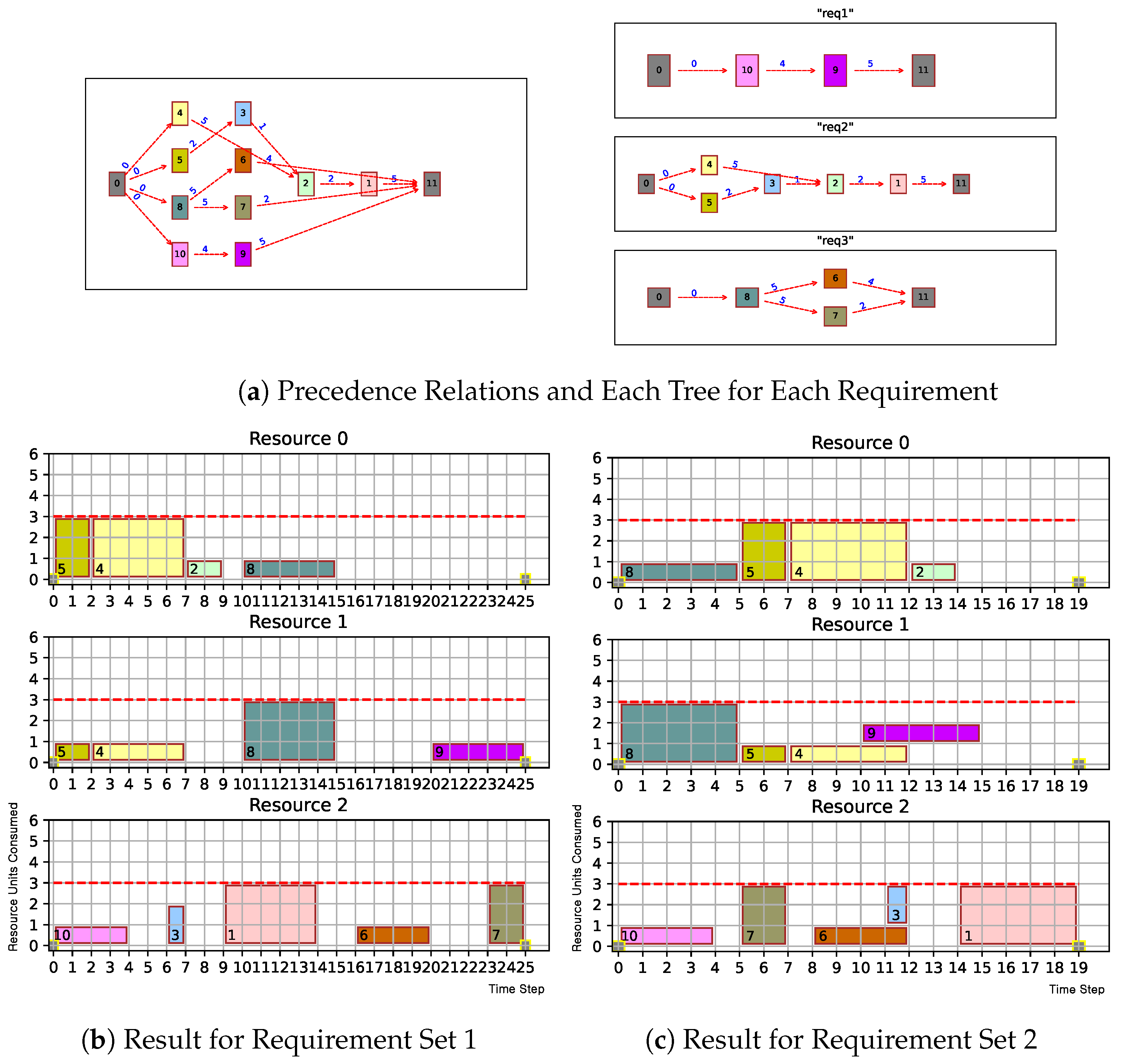
5.1. Listings of Requirements

In order to handle multiple schedules, we sequentially process each pair of inputs. Each schedule ${\mathcal{F}}_i$ consists of an instance ${\mathcal{I}}_i$ and a set of requirements ${\mathcal{R}}_i$.

${\mathcal{J}}_i$ is a tree ID in the ASP code, and ${\mathcal{F}}_i$ is a set of trees in the schedule. A $\mathtt{tree}/\mathtt{2}$ not only represents a set of relationships between related jobs but it also specifies the relationship between each tree and its respective stakeholder. Hence, we have a predicate $\mathtt{owner}/\mathtt{2}$. In the following listings, the owner represents the relationship between each requirement and its corresponding tree. Since two stakeholders may have similar requirements, we have the concept of track. Therefore, we use the predicate $\mathtt{tree}\_\mathtt{extension}/\mathtt{3}$ and $\mathtt{preferable}\_\mathtt{range}/\mathtt{4}$ to specify the same stakeholder across multiple schedules.

5.1.1. Solution for Req¹

The listing below focuses on restricting a specific tree of jobs, requested by a specific stakeholder, to ensure timely completion. For this, we give a predicate $\mathtt{deadline}/\mathtt{2}$. First, we collect the corresponding tail jobs in Equation (13). Next, before checking if the corresponding tree meets the deadline, we have to simply check the validation of the given deadline/2, comparing this with a precomputed value of the tree’s minimum duration in Equation (15). Then, in Equations (16) and (17), we check if at least one of the tail jobs is planning to finish the exact time we gave. With the constraint in Equation (14), followed by Equation (13), we can reliably conclude that all other jobs will be completed before the deadline.

$$\begin{array}{cc}\hfill \mathtt{punctual}\_\mathtt{candidate}(\mathtt{A},\mathtt{I}\mathtt{2})\leftarrow & \mathtt{task}(\mathtt{A}),\mathtt{tree}(\mathtt{TR},\mathtt{A}),\mathtt{owner}(\mathtt{“}\mathtt{req}\mathtt{1}\mathtt{”},\mathtt{TR}),\mathtt{start}(\mathtt{A},\mathtt{I}\mathtt{2}),\hfill \end{array}$$

$$\begin{array}{cc}\hfill & \mathtt{0}==\#\mathtt{count}\{\mathtt{1}:\mathtt{psrel}(\mathtt{A},\mathtt{B}),\mathtt{tree}(\mathtt{TR},\mathtt{B})\}.\hfill \\ \hfill \leftarrow & \mathtt{punctual}\_\mathtt{candidate}(\mathtt{A},\mathtt{I}\mathtt{2}),\mathtt{deadline}(\mathtt{TR},\mathtt{I}),\mathtt{dur}(\mathtt{A},\mathtt{I}\mathtt{1}),\hfill \end{array}$$

(13)

$$\begin{array}{cc}\hfill & \mathtt{tree}(\mathtt{TR},\mathtt{A}),\mathtt{I}\mathtt{2}>\mathtt{I}-\mathtt{I}\mathtt{1},\mathtt{step}(\mathtt{I}\mathtt{2}).\hfill \end{array}$$

(14)

$$\begin{array}{cc}\hfill \leftarrow & \mathtt{deadline}(\mathtt{TR},\mathtt{I}\mathtt{1}),\mathtt{min}\_\mathtt{tree}\_\mathtt{dur}(\mathtt{TR},\mathtt{I}\mathtt{2}),\mathtt{I}\mathtt{1}<\mathtt{I}\mathtt{2}.\hfill \\ \hfill \mathtt{deadline}\_\mathtt{met}(\mathtt{TR})\leftarrow & \mathtt{punctual}\_\mathtt{candidate}(\mathtt{A},\mathtt{I}\mathtt{2}),\mathtt{deadline}(\mathtt{TR},\mathtt{I}),\hfill \end{array}$$

(15)

$$\begin{array}{cc}\hfill & \mathtt{tree}(\mathtt{TR},\mathtt{A}),\mathtt{I}\mathtt{2}==\mathtt{I}-\mathtt{I}\mathtt{1},\mathtt{dur}(\mathtt{A},\mathtt{I}\mathtt{1}).\hfill \\ \hfill \leftarrow & \mathtt{C}\mathtt{1}=\#\mathtt{count}\{\mathtt{1},\mathtt{TR}:\mathtt{deadline}(\mathtt{TR},\_)\},\mathtt{C}\mathtt{1}\ne \mathtt{C}\mathtt{2},\hfill \end{array}$$

(16)

$$\begin{array}{cc}\hfill & \mathtt{C}\mathtt{2}=\#\mathtt{count}\{\mathtt{1},\mathtt{TR}:\mathtt{deadline}\_\mathtt{met}(\mathtt{TR})\}.\hfill \end{array}$$

(17)

5.1.2. Solution for Req²

The following list focuses on allocating additional resources to specific jobs for specific stakeholders. To achieve this, we provide a specific resource type, $r^{★}$, and a predicate called $\mathtt{preferable}\_\mathtt{range}/\mathtt{3}$. Firstly, in Equations (18) and (24), we classify jobs of trees that do not belong to the stakeholders of interest and/or do not require the specific resource $r^{★}$ as unoverassignable tasks. Then, we gather overassignable tasks in Equation (20) and assign an additional amount of resource $r^{★}$ in Equation (21). Through Equations (22) and (23), the assigned amount becomes no higher than the limit (Equation (23) works with Equations (10) and (11). In addition, Equation (9) is replaced with Equations (23)–(25)). Finally, with the rule in Equation (26) and its constraints in Equations (27) and (28), we can determine the total amount of excess resources allocated to the tree, keeping the value safely within the preferable range (We note that, conservatively, the lower bound of the preferred range could be zero. This is because, in some extreme cases, there may be no extra volume needed to overassign the resource. In such a scenario, the existing listing for $Re{q}^2$ may not be sufficient to meet the required range. However, we can compute the available volume early on while investigating the instance and determining the preferable range.).

$$\begin{array}{cc}\hfill \mathtt{excessed}(\mathtt{A},\mathtt{0})\leftarrow & \mathtt{task}(\mathtt{A}),\mathtt{tree}(\mathtt{TR},\mathtt{A}),\mathtt{not}\mathtt{owner}(\mathtt{“}\mathtt{req}\mathtt{2}\mathtt{”},\mathtt{TR}).\hfill \\ \hfill \mathtt{excessed}(\mathtt{A},\mathtt{0})\leftarrow & \mathtt{task}(\mathtt{A}),\mathtt{tree}(\mathtt{TR},\mathtt{A}),\mathtt{owner}(\mathtt{“}\mathtt{req}\mathtt{2}\mathtt{”},\mathtt{TR}),\hfill \end{array}$$

(18)

$$\begin{array}{cc}\hfill & \mathtt{0}==\#\mathtt{count}\{\mathtt{L}\mathtt{1}:\mathtt{rsreq}(\mathtt{A},{\mathtt{r}}^{★},\mathtt{L}\mathtt{1})\}.\hfill \\ \hfill \mathtt{overassignable}(\mathtt{A})\leftarrow & \mathtt{task}(\mathtt{A}),\mathtt{tree}(\mathtt{TR},\mathtt{A}),\mathtt{owner}(\mathtt{“}\mathtt{req}\mathtt{2}\mathtt{”},\mathtt{TR}),\hfill \end{array}$$

(19)

$$\begin{array}{cc}\hfill & \mathtt{rsreq}(\mathtt{A},{\mathtt{r}}^{★},\mathtt{L}\mathtt{1}),\mathtt{limit}({\mathtt{r}}^{★},\mathtt{L}\mathtt{2}),\mathtt{L}\mathtt{1}\le \mathtt{L}\mathtt{2}.\hfill \end{array}$$

(20)

$$\begin{array}{cc}\hfill \mathtt{1}\{\mathtt{excessed}(\mathtt{A},\mathtt{L}\mathtt{1}):\mathtt{level}(\mathtt{L}\mathtt{1})\}\mathtt{1}\leftarrow & \mathtt{overassignable}(\mathtt{A}),\mathtt{tree}(\mathtt{TR},\mathtt{A}),\mathtt{owner}(\mathtt{“}\mathtt{req}\mathtt{2}\mathtt{”},\mathtt{TR}).\hfill \\ \hfill \leftarrow & \mathtt{excessed}(\mathtt{A},\mathtt{L}\mathtt{1}),\mathtt{rsreq}(\mathtt{A},{\mathtt{r}}^{★},\mathtt{L}\mathtt{2}),\mathtt{limit}({\mathtt{r}}^{★},\mathtt{L}\mathtt{3}),\hfill \end{array}$$

(21)

$$\begin{array}{cc}\hfill & \mathtt{L}\mathtt{1}+\mathtt{L}\mathtt{2}>\mathtt{L}\mathtt{3}.\hfill \\ \hfill \mathtt{assigned}\_\mathtt{res}(\mathtt{TS},\mathtt{A},{\mathtt{r}}^{★},\mathtt{AM})\leftarrow & \mathtt{step}(\mathtt{TS}),\mathtt{overassignable}(\mathtt{A}),\mathtt{excessed}(\mathtt{A},\mathtt{L}\mathtt{1}),\hfill \\ \hfill & \mathtt{dur}(\mathtt{A},\mathtt{AD}),\mathtt{start}(\mathtt{A},\mathtt{TS}\mathtt{1}),\mathtt{TS}\mathtt{1}\le \mathtt{TS}<\mathtt{TS}\mathtt{1}+\mathtt{AD},\hfill \end{array}$$

(22)

$$\begin{array}{cc}\hfill & \mathtt{rsreq}(\mathtt{A},{\mathtt{r}}^{★},\mathtt{L}\mathtt{2}),\mathtt{AM}=\mathtt{L}\mathtt{1}+\mathtt{L}\mathtt{2}\hfill \\ \hfill \mathtt{assigned}\_\mathtt{res}(\mathtt{TS},\mathtt{A},{\mathtt{r}}^{★},\mathtt{L}\mathtt{2})\leftarrow & \mathtt{step}(\mathtt{TS}),\mathtt{not}\mathtt{overassignable}(\mathtt{A}),\mathtt{task}(\mathtt{A}),\hfill \\ \hfill & \mathtt{dur}(\mathtt{A},\mathtt{AD}),\mathtt{start}(\mathtt{A},\mathtt{TS}\mathtt{1}),\mathtt{TS}\mathtt{1}\le \mathtt{TS}<\mathtt{TS}\mathtt{1}+\mathtt{AD},\hfill \end{array}$$

(23)

$$\begin{array}{cc}\hfill & \mathtt{rsreq}(\mathtt{A},{\mathtt{r}}^{★},\mathtt{L}\mathtt{2}).\hfill \\ \hfill \mathtt{assigned}\_\mathtt{res}(\mathtt{TS},\mathtt{A},\mathtt{R},\mathtt{L}\mathtt{2})\leftarrow & \mathtt{step}(\mathtt{TS}),\mathtt{task}(\mathtt{A}),\mathtt{dur}(\mathtt{A},\mathtt{AD}),\mathtt{start}(\mathtt{A},\mathtt{TS}\mathtt{1}),\hfill \end{array}$$

(24)

$$\begin{array}{cc}\hfill & \mathtt{TS}\mathtt{1}\le \mathtt{TS}<\mathtt{TS}\mathtt{1}+\mathtt{AD},\mathtt{rsreq}(\mathtt{A},\mathtt{R},\mathtt{L}\mathtt{2}),\mathtt{R}\ne {\mathtt{r}}^{★}.\hfill \\ \hfill \mathtt{excess}\_\mathtt{in}\_\mathtt{total}(\mathtt{TR},\mathtt{AM})\leftarrow & \mathtt{preferable}\_\mathtt{range}(\mathtt{TR},\mathtt{LB},\mathtt{HB}),\hfill \end{array}$$

(25)

$$\begin{array}{cc}\hfill & \mathtt{AM}=\#\mathtt{sum}\{\mathtt{X},\mathtt{A}:\mathtt{excessed}(\mathtt{A},\mathtt{X}),\mathtt{tree}(\mathtt{TR},\mathtt{A})\}.\hfill \\ \hfill \leftarrow & \mathtt{preferable}\_\mathtt{range}(\mathtt{TR},\mathtt{LB},\mathtt{HB}),\mathtt{AM}<\mathtt{LB},\hfill \end{array}$$

(26)

$$\begin{array}{cc}\hfill & \mathtt{excess}\_\mathtt{in}\_\mathtt{total}(\mathtt{TR},\mathtt{AM}).\hfill \\ \hfill \leftarrow & \mathtt{preferable}\_\mathtt{range}(\mathtt{TR},\mathtt{LB},\mathtt{HB}),\mathtt{AM}>\mathtt{HB},\hfill \end{array}$$

(27)

$$\begin{array}{cc}\hfill & \mathtt{excess}\_\mathtt{in}\_\mathtt{total}(\mathtt{TR},\mathtt{AM}).\hfill \end{array}$$

(28)

5.1.3. Basic Solution for Req³

The following listing focuses on the overall delay for specific trees. We compute each schedule sequentially and measure this delay over the schedules by tracing the same track in Equations (29)–(31). For this inter-schedule tracking, we give three predicates: $\mathtt{delay}\_\mathtt{range}/\mathtt{1},\mathtt{delay}\_\mathtt{margin}/\mathtt{2}$, and $\mathtt{tree}\_\mathtt{extension}/\mathtt{3}$.

In addition, in order to calculate the delay (in Equations (34)–(37)), minimum tree durations for specific trees are pre-computed before scheduling. The previous schedule updates the predicate $\mathtt{delay}\_\mathtt{margin}/\mathtt{2}$ and $\mathtt{delay}\_\mathtt{range}/\mathtt{1}$. Equations (40) and (41) process the $\mathtt{delay}\_\mathtt{margin}/\mathtt{2}$ for the current schedule using the measured actual delay. The constraint in Equation (42) safely validates the actual delay for the specific tree within the overall margin.

$$\begin{array}{cc}\hfill \mathtt{tr}\_\mathtt{rel}(\mathtt{TR},\mathtt{A})\leftarrow & \mathtt{owner}(\mathtt{“}\mathtt{req}\mathtt{3}\mathtt{”},\mathtt{X}),\mathtt{tree}(\mathtt{X},\mathtt{A}),\mathtt{tree}\_\mathtt{extension}(\mathtt{TR},\mathtt{X},\_).\hfill \end{array}$$

(29)

$$\begin{array}{cc}\hfill \mathtt{tr}\_\mathtt{psrel}(\mathtt{TR},\mathtt{A},\mathtt{B})\leftarrow & \mathtt{psrel}(\mathtt{A},\mathtt{B}),\mathtt{tr}\_\mathtt{rel}(\mathtt{TR},\mathtt{A}),\mathtt{tr}\_\mathtt{rel}(\mathtt{TR},\mathtt{B}).\hfill \end{array}$$

(30)

$$\begin{array}{cc}\hfill \mathtt{tr}(\mathtt{TR})\leftarrow & \mathtt{tr}\_\mathtt{rel}(\mathtt{TR},\_).\hfill \end{array}$$

(31)

$$\begin{array}{cc}\hfill \mathtt{heads}(\mathtt{TR},\mathtt{A})\leftarrow & \mathtt{tr}\_\mathtt{rel}(\mathtt{TR},\mathtt{A}),\mathtt{0}==\#\mathtt{count}\{\mathtt{1}:\mathtt{tr}\_\mathtt{psrel}(\mathtt{TR},\mathtt{B},\mathtt{A})\}.\hfill \end{array}$$

(32)

$$\begin{array}{cc}\hfill \mathtt{tails}(\mathtt{TR},\mathtt{A})\leftarrow & \mathtt{tr}\_\mathtt{rel}(\mathtt{TR},\mathtt{A}),\mathtt{0}==\#\mathtt{count}\{\mathtt{1}:\mathtt{tr}\_\mathtt{psrel}(\mathtt{TR},\mathtt{A},\mathtt{B})\}.\hfill \end{array}$$

(33)

$$\begin{array}{cc}\hfill \mathtt{min}\_\mathtt{tree}\_\mathtt{duration}(\mathtt{TR},\mathtt{I})\leftarrow & \mathtt{tree}\_\mathtt{extension}(\mathtt{TR},\mathtt{X},\_),\mathtt{min}\_\mathtt{tree}\_\mathtt{dur}(\mathtt{X},\mathtt{I}).\hfill \\ \hfill \mathtt{actual}\_\mathtt{tree}\_\mathtt{duration}(\mathtt{TR},\mathtt{I}\mathtt{3})\leftarrow & \mathtt{I}\mathtt{1}=\#\mathtt{min}\{\mathtt{I}:\mathtt{start}(\mathtt{A},\mathtt{I}),\mathtt{heads}(\mathtt{TR},\mathtt{A})\},\mathtt{tr}(\mathtt{TR}),\hfill \\ \hfill & \mathtt{I}\mathtt{2}=\#\mathtt{max}\{\mathtt{I}+\mathtt{D}:\mathtt{start}(\mathtt{B},\mathtt{I}),\mathtt{dur}(\mathtt{B},\mathtt{D}),\mathtt{tails}(\mathtt{TR},\mathtt{B})\},\hfill \end{array}$$

(34)

$$\begin{array}{cc}\hfill & \mathtt{I}\mathtt{3}+\mathtt{I}\mathtt{1}==\mathtt{I}\mathtt{2},\mathtt{I}\mathtt{1}<\mathtt{I}\mathtt{2},\mathtt{step}(\mathtt{I}\mathtt{3}).\hfill \\ \hfill \mathtt{actual}\_\mathtt{delay}(\mathtt{TR},\mathtt{L}\mathtt{3})\leftarrow & \mathtt{min}\_\mathtt{tree}\_\mathtt{duration}(\mathtt{TR},\mathtt{L}\mathtt{1}),\mathtt{actual}\_\mathtt{tree}\_\mathtt{duration}(\mathtt{TR},\mathtt{L}\mathtt{2}),\hfill \end{array}$$

(35)

$$\begin{array}{cc}\hfill & \mathtt{L}\mathtt{3}+\mathtt{L}\mathtt{1}==\mathtt{L}\mathtt{2},\mathtt{L}\mathtt{1}\le \mathtt{L}\mathtt{2},\mathtt{delay}\_\mathtt{range}(\mathtt{L}\mathtt{3}).\hfill \end{array}$$

(36)

$$\begin{array}{cc}\hfill \leftarrow & \mathtt{0}==\#\mathtt{count}\{\mathtt{1}:\mathtt{actual}\_\mathtt{delay}(\mathtt{TR},\mathtt{L}\mathtt{3})\}.\hfill \\ \hfill \mathtt{within}\_\mathtt{delay}\_\mathtt{range}(\mathtt{TR},\mathtt{CD}\mathtt{1})\leftarrow & \mathtt{tree}\_\mathtt{extension}(\mathtt{TR},\_,\mathtt{L}\mathtt{1}),\mathtt{actual}\_\mathtt{delay}(\mathtt{TR},\mathtt{L}\mathtt{2}),\hfill \end{array}$$

(37)

$$\begin{array}{cc}\hfill & \mathtt{L}\mathtt{1}==\mathtt{L}\mathtt{2}+\mathtt{CD}\mathtt{1},\mathtt{delay}\_\mathtt{range}(\mathtt{CD}\mathtt{1}).\hfill \\ \hfill \mathtt{outside}\_\mathtt{delay}\_\mathtt{range}(\mathtt{TR},\mathtt{CD}\mathtt{1})\leftarrow & \mathtt{tree}\_\mathtt{extension}(\mathtt{TR},\_,\mathtt{L}\mathtt{1}),\mathtt{actual}\_\mathtt{delay}(\mathtt{TR},\mathtt{L}\mathtt{2}),\hfill \end{array}$$

(38)

$$\begin{array}{cc}\hfill & \mathtt{L}\mathtt{1}+\mathtt{CD}\mathtt{1}==\mathtt{L}\mathtt{2},\mathtt{CD}\mathtt{1}\ge \mathtt{1},\mathtt{delay}\_\mathtt{range}(\mathtt{CD}\mathtt{1}).\hfill \\ \hfill \mathtt{current}\_\mathtt{delay}\_\mathtt{margin}(\mathtt{TR},\mathtt{CD}\mathtt{2})\leftarrow & \mathtt{outside}\_\mathtt{delay}\_\mathtt{range}(\mathtt{TR},\mathtt{CD}\mathtt{1}),\mathtt{delay}\_\mathtt{margin}(\mathtt{TR},\mathtt{CD}),\hfill \end{array}$$

(39)

$$\begin{array}{cc}\hfill & \mathtt{CD}\mathtt{1}+\mathtt{CD}\mathtt{2}==\mathtt{CD},\mathtt{CD}\mathtt{2}\le \mathtt{CD},\mathtt{CD}\mathtt{1}\le \mathtt{CD},\mathtt{delay}\_\mathtt{range}(\mathtt{CD}\mathtt{2}).\hfill \\ \hfill \mathtt{current}\_\mathtt{delay}\_\mathtt{margin}(\mathtt{TR},\mathtt{CD}\mathtt{2})\leftarrow & \mathtt{within}\_\mathtt{delay}\_\mathtt{range}(\mathtt{TR},\mathtt{CD}\mathtt{1}),\mathtt{delay}\_\mathtt{margin}(\mathtt{TR},\mathtt{CD}),\hfill \end{array}$$

(40)

$$\begin{array}{cc}\hfill & \mathtt{CD}\mathtt{1}+\mathtt{CD}==\mathtt{CD}\mathtt{2},\mathtt{delay}\_\mathtt{range}(\mathtt{CD}\mathtt{2}).\hfill \\ \hfill \leftarrow & \mathtt{tree}\_\mathtt{extension}(\mathtt{TR},\_,\mathtt{L}\mathtt{1}),\mathtt{actual}\_\mathtt{delay}(\mathtt{TR},\mathtt{L}\mathtt{2}),\hfill \end{array}$$

(41)

$$\begin{array}{cc}\hfill & \mathtt{delay}\_\mathtt{margin}(\mathtt{TR},\mathtt{L}\mathtt{3}),\mathtt{L}\mathtt{2}-\mathtt{L}\mathtt{3}>\mathtt{L}\mathtt{1}.\hfill \end{array}$$

(42)

5.2. Combining Listings with Procedural Codes

To satisfy all specified requirements, particularly $Re{q}^2$ and $Re{q}^3$, it is necessary to compute all schedules within the set of job forests ${\mathcal{F}}_1,{\mathcal{F}}_2,\dots$. The procedure to calculate these schedules is as follows:

Algorithm 1 outlines the procedural flow for solving a sequence of vertiport scheduling instances, each with associated stakeholder requirements. This procedure corresponds to the simple flow depicted in Figure 2a in Section 4.2. For each instance and requirement pair $\langle {\mathcal{I}}_i,{\mathcal{R}}_i\rangle$ (We remark that the instance $\mathcal{I}$ has predicates related to task, tree, precedence relationship, required resources, and their limits. The requirement $\mathcal{R}$ has predicates related to the deadline of some trees, the preferable amount of resources and their quarters, and permitable track and tree extensions. Auxiliary facts are predicates related to the time step range, resource levels, dummy tasks and their precedence relationships, delay range and margin, and minimum tree durations for some trees.) in the input list, along with its current delay margin $\mathcal{M}\left[i\right]$ (The delay margin, $\mathcal{M}$, is for $Re{q}^3$. When the corresponding tree takes longer than its minimum duration, it represents an allowable delay. Therefore, during the sequential schedule calculation, we measure the tree’s delay and update the allowable margin accordingly. In Algorithm 2, we show how to handle this from outside, including its setup.), the algorithm initializes a reasoning controller, $\mathcal{C}$. This controller is then loaded with the foundational RCPSP rules (Equations (7)–(12)), the specific ASP rules for handling stakeholder requirements (Equations (13)–(42)), the factual data representing the current scheduling instance ${\mathcal{I}}_i$ and its requirements ${\mathcal{R}}_i$, any necessary auxiliary facts, and the current delay margin $\mathcal{M}\left[i\right]$. The $\mathcal{C}.ground()$ operation translates these rules and facts into a propositional program suitable for the ASP solver. Subsequently, $\mathcal{C}.compute()$ invokes the solver to find an optimal schedule. If a satisfiable model is found ($\mathcal{C}.satisfiable()$ is true), the resulting schedule ${\mathcal{S}}_i$ and the outcome of the requirement satisfaction ${\mathcal{R}}_i^{\mathcal{S}}$ are extracted from $\mathcal{C}.model()$. This pair is stored, and then the delay margin list is updated to $\mathcal{M}[i+1]$ based on the current_delay_margin/2 predicate, which is derived from the model. This is for use in the next iteration or by a higher-level iterative process (We note that for the last iteration, where the returned model is for the last schedule and its requirement, the delay margin in the first index is updated. For further details, refer to Algorithm 2, where each iteration requires the updated $\mathcal{M}$ for the RCPSP-REQ-ASP.). While sequentially processing all input pairs, it returns the list of computed schedules and the final updated delay margins.

Algorithm 1: RCPSP-REQ-ASP

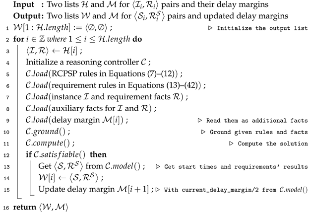Algorithm 2: RCPSP-REQ-ASP-ITER

Algorithm 2 describes an iterative approach to handle interdependencies between schedules. This is particularly for serving requirements like $Re{q}^3$ that involve managing delays across a series of operations. This procedure aligns with the ’Iterative Approach’ shown in Figure 2a in Section 4.2. The algorithm first initializes a list of delay margins $\mathcal{M}$ to zeros for all trees in the input instances. It then starts a while loop. This loop continues as long as the progressing holds (by which the flag keeps true). Within the loop, it calls Algorithm 1. The current set of instances $\mathcal{H}$ and the delay margins $\mathcal{M}$ are delivered to the input. Algorithm 1 then returns the computed schedules $\mathcal{W}$ and potentially updated margins $\mathcal{M}$. The termination condition, CheckTerminationCondition($\mathcal{W}$) (as defined in Equation (43)), is evaluated. This condition check investigates if the set of schedules $\mathcal{W}$ has changed. If $\mathcal{W}$ has changed, it repeats the iteration again. However, if $\mathcal{W}$ has stabilized (i.e., no changes occurred), the terminated flag becomes true. This makes progressing false, and the loop terminates. It finally returns the final set of computed schedules $\mathcal{W}$. This procedure allows schedules to adjust based on the outcomes and delay propagations from others.

$$\mathrm{CHECK}\mathrm{TERMINATION}\mathrm{CONDITION}(\mathcal{W}):=\left\{\begin{array}{cc}False\hfill & \mathcal{W}\mathrm{is}\mathrm{changed}\hfill \\ True\hfill & \mathrm{otherwise}\hfill \end{array}\right.$$

(43)

Remark on Termination Condition: In our practical implementation, the termination condition specified in Equation (43) is adjusted to handle intrinsic cycles. In Algorithm 2, we terminate the iteration process if terminated becomes true as a result of having ‘not changed’. We regard having ‘not changed’ when the current set of schedules $\mathcal{W}$ matches any set of schedules $\mathcal{W}$ that has been generated in a previous iteration. On the other hand, the process is considered ‘changed’ if the current $\mathcal{W}$ is novel compared to all previously generated sets. This approach ensures termination even if the algorithm enters a cycle of states rather than strictly converging to a fixed point identical to the immediately preceding iteration, a behavior observed in a small percentage (less than 1%) of our test instances. It is important to note that this convergence process is not related to optimizing each job forest but to finding stable, balanced delay margins over the set of job forests.

Theorem 1

(Correctness). Each listing for $Re{q}^k$, where $k\in \{1,2,3\}$, restricts an instance $\mathcal{I}$ as it is specified in $\mathcal{R}$.

Proof. 

We have three cases for the entire set of requirements.

Case $k=1$ s.t. $Re{q}^1$: The $\mathcal{R}$ is deadline/2. We demonstrate here that the corresponding tree’s task does not exceed the given deadline, and the tree meets the deadline. First of all, Equation (15) guarantees the validity of the given deadline, comparing the deadline of the corresponding tree with its precomputed minimum duration. Next, given that the puctual_candidate/2 collects the tail jobs in the related tree and applies the constraint in Equation (14), it is valid to say that no subsequent job will start after the deadline. The rule for deadline_met/1 in Equation (16) and the constraint in Equation (17) require at least one tail job to finish at deadline/2. Therefore, in order to satisfy the model, the constraints should hold, making the latest tail job be finished on time.

Case $k=2$ s.t. $Re{q}^2$: The $\mathcal{R}$ comprises two elements: $r^{★}$ and preferable_range/3. Here, we demonstrate that it only selects $r^{★}$ requiring tasks as overassignable tasks in the corresponding tree and ensures that the total amount of overassigned resources does not fall below or exceed the preferred range. First, constraints in Equations (18) and (24) remove irrelevant tasks, assigning zero to the excess value. These tasks in the corresponding tree have no effect on the total. Secondly, the rule in Equation (20) gathers relevant tasks, and Equations (21) and (22) provide possibly permitted excess values. Finally, the constraints in Equations (27) and (28) force the computed total amount of excessed values over the tasks in Equation (26) to fall within the specified preference range.

Case $k=3$ s.t. $Re{q}^3$: The $\mathcal{R}$ consists of delay_range/2, delay_margin/2, and tree_extension/3. Here, we demonstrate that the actual delays for trees in the corresponding track do not surpass the limits set by $\mathcal{R}$. Firstly, to select the same track, we obtain the track value from tree_extension/3 in Equation (29). Then, for all the other rules representing the variable TR, we use the track value. Secondly, after measuring an actual tree duration and comparing it with its minimum duration in Equations (34) and (35), it computes the actual delay. Finally, it computes the current delay margin, taking into account both the actual delay and the given delay margin. The constraint in Equation (42) ensures that the actual delay, when subtracted by the given margin, should not surpass the tree_extension/3, thereby controlling the start times for corresponding heads and tails within this boundary. This ensures that the actual tree duration and delay do not exceed the extension.    □

Theorem 2

(Completeness). Given a sequence of $〈\mathcal{I},\mathcal{R}〉$ pairs as the input of the RCPSP-REQ problem, Algorithm 2 computes a sequence of schedules if one exists and outputs the computed schedules with the results of requirements if one exists. Otherwise, it returns an empty set.

Proof. 

In this proof, both cases are covered:

The first case is whether Algorithm 2 computes a solution when one exists. Without loss of generality, the existing solution has a form of $\mathcal{W}$, which consists of $\mathcal{S}$ and ${\mathcal{R}}^{\mathcal{S}}$ pairs. Additionally, each element pair in $\mathcal{W}$ has been updated with a proper schedule and a result based on the requirements, replacing the initial empty set. Since each iteration in Algorithm 2 calls Algorithm 1, and Algorithm 1 returns $〈\mathcal{W},\mathcal{M}〉$ without any exception, we can safely obtain the result from Algorithm 1. The only case when one of the output pairs has the un-updated element from its initial value is that the model from the controller $\mathcal{C}$ is not satisfied in line 12 of Algorithm 1. Therefore, a successful element pair with the proper schedule and a requirements’ result implies that it holds all rules and constraints in RCPSP and the requirements in Equations (7)–(42), returning a model that is a set of start times for tasks and requirement results. Then, this iteration in Algorithm 2 repeats until the termination condition in line 5 is met. Finally, it exits the loop, returning the $\mathcal{W}$ output.

The second case is whether it returns an empty set when a solution does not exist. Assume that one of the instance and requirement pairs does not have a solution. We can easily elaborate on this case. Without loss of generality, the failed output has an empty set, and this set has a form of $〈\varnothing ,\varnothing 〉$ by its initial setup in line 1 in Algorithm 1. Since this input, which we refer to as ${\mathcal{I}}^{\perp }$ here, lacks a proper schedule, we are unable to determine a set of start times for tasks within ${\mathcal{I}}^{\perp }$. We assume that there exists an unempty set of tasks in ${\mathcal{I}}^{\perp }$. If it has an empty set of tasks, still it cannot satisfy the requirements (i.e., the deadline/2) so that it is unsatisfiable, returning an empty set as its output. Since this unempty set of tasks does not have a set of start times; this cannot meet the requirements. For example, there is no set of start times to satisfy the deadline/2 in $Re{q}^1$. Hence, it is not satisfiable in line 12 in Algorithm 1, keeping the initial value the same. Algorithm 2 repeats this iteration, maintaining the same value for this element without any changes. This holds the termination condition, and then finally, it returns an empty set of the element in the output list.    □

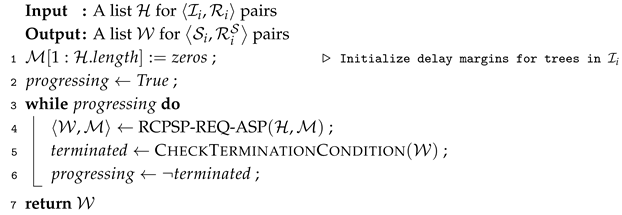6. Experiments and Discussions

6.1. Experiments

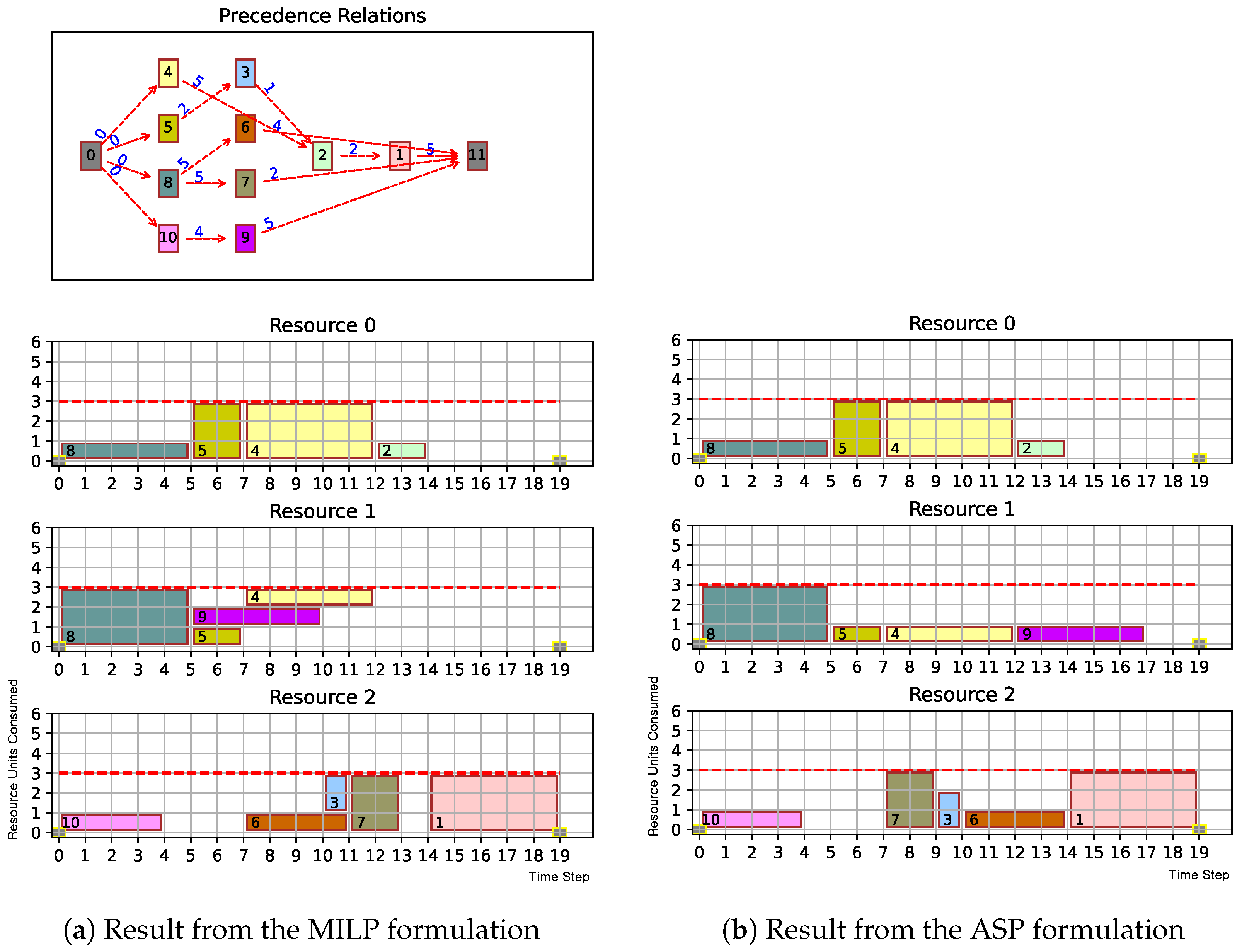
6.1.1. Toy Example

To demonstrate the conceptual example of our solution, we examined the same instance in Table 1.

Table 3. Facts and Results for $\mathcal{R}$ set 1 and $\mathcal{R}$ set 2.

	$\mathcal{R}$ Set 1	$\mathcal{R}$ Set 2
Aux. facts for $\mathcal{I}$	The set $\mathcal{F}$ is {“tx1”, “tx2”, “tx3”}. owner(“req1”, “tx3”), owner(“req2”, “tx1”), owner(“req3”, “tx2”), tree(“tx3”, 9..10), tree(“tx1”, 1..5), tree(“tx2”, 6..8).
Aux. facts for $\mathcal{R}$	deadline(“tx3”, 25), preferable_range(“tx1”, 1, 2), text_extension(0, “tx2”, 5), delay_range(0..5).	deadline(“tx3”, 15), preferable_range(“tx1”, 2, 3), text_extension(0, “tx2”, 4), delay_range(0..4).
Additional facts	delay_margin(0, 0).
$Re{q}^1$	punctual_candidate(9, 20), deadline_met(“tx3”).	punctual_candidate(9, 10), deadline_met(“tx3”).
$Re{q}^2$	excessed(4, 1), excessed(5, 1), excess_in_total(0, 2).	excessed(4, 1), excessed(5, 1), excess_in_total(0, 2).
$Re{q}^3$	actual_delay(0, 4).	actual_delay(0, 1).
Total Duration	estart(25).	estart(19).

represents the facts given for two different requirement sets and their results. Figure 3 shows individual trees for the owners of $Re{q}^1$, $Re{q}^2$, and $Re{q}^3$ and resource assignments for each requirement set.

Both sets have a common auxiliary fact for the constraint: $\mathcal{I}$. $\mathcal{R}$ set 1 has a deadline at 25 steps, while $\mathcal{R}$ set 2 has a deadline at 15 steps. The preferable ranges for the overassignable resource are 1 to 2, 2 to 3, respectively. $\mathcal{R}$ set 1 allows the extensions of the tree to span up to five steps, while $\mathcal{R}$ set 2 allows it up to four steps. Both sets were configured with no allowable delay margin (set to zero). For $Re{q}^1$, task 9 ends at 25 steps in Figure 3b and ends at 15 steps in Figure 3c. For $Re{q}^2$, both have one unit of the excess resource for tasks 4 and 5 (Refer to the excessed/2 in the $Re{q}^2$ row of Table 3. In addition, in this example, $r^{★}$ is Resource 1.). The available slots range from 0 to 7 steps in Figure 3b and from 5 to 12 steps in Figure 3c. For $Re{q}^3$, the actual tree durations for the tree are 15 steps and 12 steps, respectively.

6.1.2. Numerical Experiments

We constructed a common experimental environment, using exclusively open-source software to ensure full reproducibility. The MILP models were implemented through Python (version 3.12.3, conda-forge, AMD64). We used the PuLP library (version 2.8.0) with the CBC (COIN-OR Branch and Cut) solver, accessed via PULP_CBC_CMD, running within a Cygwin environment. For the ASP-based approaches, we used Clingo (version 5.7.1). This is also operated within the same Python environment as the MILP experiments. For the experiments, the machine we used had an 11th Gen Intel(R) Core(TM) i5-1135G7 processor (Intel Corporation, Santa Clara, CA, USA) at 2.40 GHz and 8GB of RAM. A consistent time limit of 600 s was set for each instance across both cases.

We constructed a common experimental environment. The MILP models were implemented through Python (version 3.12.3; Python Software Foundation, Wilmington, DE, USA). We used the PuLP library (version 2.8.0; University of Auckland, Auckland, New Zealand) with the CBC (COIN-OR Branch and Cut) solver (COIN-OR Foundation, Towson, MD, USA), running within a Cygwin environment (Red Hat, Inc., Raleigh, NC, USA). For the ASP-based approaches, we used Clingo (version 5.7.1; University of Potsdam, Potsdam, Germany). This is also operated within the same Python environment as the MILP experiments. The machine we used had an 11th Gen Intel(R) Core(TM) i5-1135G7 processor (Intel Corporation, Santa Clara, CA, USA) at 2.40 GHz and 8GB of RAM. A consistent time limit of 600 s was set for each instance across both cases.

Within this setup, we conducted two major numerical experiments. The first experiment evaluates scalability for both approaches and assesses solution time for standard RCPSP instances.

Table 4. Numerical Results for MILP vs. ASP. Time [s] denotes the computation time in seconds. Step [#] indicates the makespan as the number of time steps, and Succ. [#] represents the count of successful instances.

	MILP			ASP
$\left|\mathcal{J}\right|$	${\mathcal{F}}_{\mathbf{i}}$ Time [s]	$\mathcal{S}$ Step [#]	Succ. [#]	${\mathcal{F}}_{\mathbf{i}}$ Time [s]	$\mathcal{S}$ Step [#]	Succ. [#]
	(Min|Median|Max)	(Min|Median|Max)		(Min|Median|Max)	(Min|Median|Max)
10	00.108|000.256|041.252	09|16.0|25	100	0.000|000.031|000.064	09|16.0|25	100
20	00.646|015.134|455.195	13|21.0|32	94	0.080|000.271|002.156	13|20.5|32	100
30	27.312|132.038|424.036	20|23.5|30	20	0.459|001.887|375.537	18|26.0|42	98
40	—	—	0	2.516|026.192|572.800	20|31.0|38	71
50	—	—	0	7.943|148.850|554.881	28|35.0|42	24

shows the comparison between MILP and ASP performance. In the table, ‘$\left|\mathcal{J}\right|$’ denotes the job count. ‘${\mathcal{F}}_i$ Time [s]’ indicates the minimum, median, and maximum computation time per 100 instances. ‘$\mathcal{S}$ Step [#]’ represents the minimum, median, and maximum makespan. ‘Succ. [#]’ lists successful instances (out of 100) within a 600-s limit. The results in Table 4 showed MILP’s success dropped to zero for 40 or more jobs, while ASP, though its success also declined with increasing job numbers, solved more instances for larger job sets, practically handling up to 50 jobs within our settings.

The second experiment investigated ASP with stakeholder requirements, using 100 job forests ($\mathcal{F}\mathrm{s}$), each containing five 20-job schedules (${\mathcal{F}}_i\mathrm{s}$).

Table 5. Numerical Results for Plain vs. Req vs. Iter. Time [s] is the computation time in seconds, Step [#] is the makespan in time steps, and Punctuality [#] is the count of instances meeting all punctuality requirements.

	${\mathcal{F}}_{\mathit{i}}$ Time [s]	$\mathcal{F}$ Time [s]	$\mathcal{S}$ Step [#]	Punctuality [#]
	(Min|Median|Max)	(Min|Median|Max)	(Min|Median|Max)
Plain	0.095|0.446|30.191	—	13|21|40	35
Req	0.136|0.657|04.082	01.795|03.378|08.275	16|25|45	1000
Iter	0.121|0.648|04.285	06.669|13.864|35.994	16|25|45	1000

compares the ‘Plain’, ‘Req’, and ‘Iter’ methods. In this table, ‘${\mathcal{F}}_i$ Time [s]’ shows aggregated minimum, median, and maximum computation time per individual schedule ${\mathcal{F}}_i$. ‘$\mathcal{F}$ Time [s]’ is the total computation time per complete job forest $\mathcal{F}$. ‘$\mathcal{S}$ Step [#]’ is the makespan per $\mathcal{F}$. ‘Punctuality [#]’ counts the job forests meeting all $Re{q}^1$ (punctuality requirements). Key findings, presented in Table 5 and Figure 4, include the following: The ‘Plain’ solver (Figure 4a,b, tracks 0, 2) showed no excess resource allocation and no delay limits. The ‘Req’ solver (tracks 1, 3) accommodated these. The ‘Req’ and ‘Iter’ solvers showed similar excess resource results (Figure 4c). However, the ‘Iter’ solver achieved narrower, more constrained delay ranges (Figure 4d), although its computation time was approximately four times longer than the ‘Req’ approach, reflecting its iterative refinement. The ‘Plain’ solver did not address punctuality, unlike the ‘Req’ and ‘Iter’ methods.

6.2. Discussions

6.2.1. Performance Issue

Scalability: The inherent combinatorial explosion of RCPSP limits the scalability of our solution, as demonstrated in Table 4. We recommend developing a heuristic algorithm for practical use and to support large-scale job scheduling, such as a genetic algorithm (GA) [43,44,47], differential evolution (DE) [45,46], and metaheuristic [48].

MILP vs. ASP: Comparing general computational efficiency between MILP and ASP is beyond the scope of this paper. This is because of the inherent complexities of their distinct solving paradigms. Choosing a method to solve a problem often depends on the specific problem structure. ASP solvers uses grounding techniques and conflict-driven clause learning (CDCL) similar with SAT solvers. These choices allow us to excel in problems with intricate logical constraints [71,72]. On the other hand, MILP solvers are mostly optimized for problems that fit in their linear algebraic framework. Then, they utilize methods like branch-and-cut [73,74].

The authors in [75] show that ASP-based approaches can offer competitive performance. Their statement only holds for certain types of problems, like scheduling and combinatorial optimization of their domain. In semiconductor manufacturing, their work shows that constraint answer set programming (CASP) is more effective than traditional MILP solutions. Their approach particularly generates optimal schedules for automated wet-etch stations. CASP reduces the makespan more effectively. This clearly provides that ASP is able to assist with task scheduling jobs. Even though theoretical advantages have not been proven universally, the result is consistent with what we discovered in this paper.

6.2.2. What We Have Not Covered Here

• LP Relaxation: Our approach to RCPSP is focused on MILP, not linear programming. This is because our MILP formulation in Section 3.2 was to clearly introduce discrete and countable resource management through integer programming. We can narrow down the possible result sets for a specific RCPSP case. This can be performed by heuristically performing LP relaxation. We can also establish lower bounds [38,76,77,78,79]. However, we chose MILP to obtain an exact solution. Choosing MILP let us easily transition to the ASP formulation, and this allowed for a simpler representation of the requirements.
• Graph-Based Algorithmic Approach: This scheduling problem differs from a simple pathfinding problem in that it does not involve navigating a physical environment. Decisions made in one job plan by the RCPSP will impact other job plans. This approach is quite similar to cooperative pathfinding [49]. Since this perspective is relatively new in research, we need more scenarios and simulation results. This will help us apply this problem and approach in practice.

6.2.3. Future Directions

We need to explore more detailed resource characteristics and specialized task types, such as time-varying or preemptive maintenance scheduling.

Research into human–machine interaction for UAM system operators and managers would be important to expand. This is particularly important for the decision making in automated scheduling environments.

The next step to move should be to extend and to validate our method to more complex and larger-scale UAM scheduling problems. Particularly, this includes handling real-time data (e.g., weather, congestion), integrating with broader UAM ecosystem simulations, and modeling network effects across interconnected vertiports.

In order to support the UAM vision of widespread unmanned autonomous flight and responsive on-demand services, future research ultimately should develop adaptive and resilient scheduling methodologies. These would be capable of managing dynamic and disruptive scenarios, such as priority flights or unforeseen system-wide perturbations.

7. Conclusions

This paper studies a new framework for UAM scheduling. It integrates stakeholder needs into the RCPSP via the ASP approach. Through experiments, we show that the ASP-based model outperforms traditional MILP formulations in scalability for large-scale UAM scheduling, particularly in dynamic resource allocation scenarios. Our model, then, introduces how to handle stakeholder-specific constraints, such as on-time guarantees, overassignable resources, and flexible delay bounds. This approach enables schedules that balance operational efficiency with real-world stakeholder needs and maintains feasibility while accommodating diverse requirements.

We believe that our findings are relevant to UAM operators and policymakers because this approach allows vertiports to handle increasing eVTOL traffic without sacrificing computational tractability. On the other hand, the suggested model still assumes static stakeholder priorities and, therefore, requires further investigation. Future research directions include extending the ASP formulation to handle dynamic stakeholder priorities, investigating hybrid models, optimizing multi-vertiport coordination, and incorporating energy consumption models for eVTOLs.

References

- Patterson, M.D.; Antcliff, K.; Kohlman, L.W. A Proposed Approach to Studying Urban Air Mobility Missions Including an Initial Exploration of Mission Requirements. In Proceedings of the AHS International 74th Annual Forum and Technology Display, Phoenix, AZ, USA, 15–17 May 2018. [Google Scholar] [CrossRef]
- Arafat, M.Y.; Pan, S. Urban Air Mobility Communications and Networking: Recent Advances, Techniques, and Challenges. Drones 2024, 8, 702. [Google Scholar] [CrossRef]
- Hui, K.Y.; Nguyen, C.H.; Lui, G.N.; Liem, R.P. AirTrafficSim: An Open-Source Web-Based Air Traffic Simulation Platform. J. Open Source Softw. 2023, 8, 4916. [Google Scholar] [CrossRef]
- Al–Rubaye, S.; Tsourdos, A.; Namuduri, K. Advanced Air Mobility Operation and Infrastructure for Sustainable Connected eVTOL Vehicle. Drones 2023, 7, 319. [Google Scholar] [CrossRef]
- Wild, G. Urban Aviation: The Future Aerospace Transportation System for Intercity and Intracity Mobility. Urban Sci. 2024, 8, 218. [Google Scholar] [CrossRef]
- Thipphavong, D.P.; Apaza, R.D.; Barmore, B.; Battiste, V.; Burian, B.K.; Dao, Q.; Feary, M.; Go, S.; Goodrich, K.H.; Homola, J.; et al. Urban Air Mobility Airspace Integration Concepts and Considerations. In Proceedings of the 18th AIAA Aviation Technology, Integration, and Operations Conference, Atlanta, GA, USA, 25–29 June 2018. [Google Scholar] [CrossRef]
- Hoffmann, R.; Pereira, D.P.; Nishimura, H. Security Viewpoint and Resilient Performance in the Urban Air Mobility Operation. IEEE Open J. Syst. Eng. 2023, 1, 123–138. [Google Scholar] [CrossRef]
- Gutjahr, W.J. Bi-Objective Multi-Mode Project Scheduling Under Risk Aversion. Eur. J. Oper. Res. 2015, 246, 421–434. [Google Scholar] [CrossRef]
- Fahmy, A. Optimization Algorithms in Project Scheduling. In Optimization Algorithms-Methods and Applications; IntechOpen: London, UK, 2016. [Google Scholar] [CrossRef]
- Koné, O.; Artigues, C.; Lopez, P.; Mongeau, M. Comparison of Mixed Integer Linear Programming Models for the Resource-Constrained Project Scheduling Problem with Consumption and Production of Resources. Flex. Serv. Manuf. J. 2012, 25, 25–47. [Google Scholar] [CrossRef]
- Rabbani, M.; Arjmand, A.; Saffar, M.M.; Jalali, M.S. Application of Three Meta-Heuristic Algorithms for Maximizing the Net Present Value of a Resource-Constrained Project Scheduling Problem with Respect to Delay Penalties. Int. J. Appl. Ind. Eng. 2016, 3, 1–15. [Google Scholar] [CrossRef]
- Gebser, M.; Schaub, T. Modeling and Language Extensions. AI Mag. 2016, 37, 33–44. [Google Scholar] [CrossRef]
- Fuscà, D.; Germano, S.; Zangari, J.; Anastasio, M.; Calimeri, F.; Perri, S. A Framework for Easing the Development of Applications Embedding Answer Set Programming. In Proceedings of the 18th International Symposium on Principles and Practice of Declarative Programming (PPDP), Edinburgh, UK, 5–7 September 2016. [Google Scholar] [CrossRef]
- Egly, U.; Gaggl, S.A.; Woltran, S. Answer-Set Programming Encodings for Argumentation Frameworks. Argum. Comput. 2010, 1, 147–177. [Google Scholar] [CrossRef]
- Kaufmann, B.; Leone, N.; Perri, S.; Schaub, T. Grounding and Solving in Answer Set Programming. AI Mag. 2016, 37, 25–32. [Google Scholar] [CrossRef]
- Kim, J.; Kim, K. Agent 3, change your route: Possible conversation between a human manager and UAM Air Traffic Management (UATM). In Proceedings of the Robotics: Science and Systems (RSS) workshop on Articulate Robots: Utilizing Language for Robot Learning, Daegu, Republic of Korea, 10–14 July 2023. [Google Scholar] [CrossRef]
- Kim, J.; Kim, K. Dialogue Possibilities between a Human Supervisor and UAM Air Traffic Management: Route Alteration. Adv. Artif. Intell. Mach. Learn. (AAIML) 2023, 3, 1352–1368. [Google Scholar] [CrossRef]
- Woo, S.; Kim, J.; Kim, K. We, Vertiport 6, are temporarily closed: Interactional Ontological Methods for Changing the Destination. In Proceedings of the IEEE RO-MAN (RO-MAN 2023) Workshop on Ontologies for Autonomous Robotics (RobOntics), Busan, Republic of Korea, 28–31 August 2023. [Google Scholar] [CrossRef]
- Kim, J.; Kim, K. Designing Reactive Route Change Rules with Human Factors in Mind: A UATM System Perspective. In Proceedings of the International Congress on Information and Communication Technology, London, UK, 19–22 February 2024; pp. 323–338. [Google Scholar] [CrossRef]
- Prakasha, P.S.; Papantoni, V.; Nagel, B.; Brand, U.; Vogt, T.; Naeem, N.; Ratei, P.; Villacis, S.P. Urban Air Mobility Vehicle and Fleet-Level Life-Cycle Assessment Using a System-of-Systems Approach. In Proceedings of the AIAA AVIATION 2021 FORUM, Virtual Event, 2–6 August 2021. [Google Scholar] [CrossRef]
- Goodrich, K.H.; Barmore, B. Exploratory Analysis of the Airspace Throughput and Sensitivities of an Urban Air Mobility System. In Proceedings of the 2018 Aviation Technology, Integration, and Operations Conference, Atlanta, GA, USA, 25–29 June 2018. [Google Scholar] [CrossRef]
- Kotwicz Herniczek, M.T.; German, B. Impact of Airspace Restrictions on Urban Air Mobility Airport Shuttle Service Route Feasibility. Transp. Res. Rec. J. Transp. Res. Board 2022, 2676, 689–706. [Google Scholar] [CrossRef]
- Vascik, P.D.; Hansman, R.J. Evaluating the Interoperability of Urban Air Mobility Systems and Airports. Transp. Res. Rec. J. Transp. Res. Board 2021, 2675, 1–14. [Google Scholar] [CrossRef]
- Vascik, P.D.; Hansman, R.J. Scaling Constraints for Urban Air Mobility Operations: Air Traffic Control, Ground Infrastructure, and Noise. In Proceedings of the 2018 Aviation Technology, Integration, and Operations Conference, Atlanta, GA, USA, 25–29 June 2018. [Google Scholar] [CrossRef]
- Dai, W.; Low, K.H. Conflict-Free Trajectory Planning for Urban Air Mobility Based on an Airspace-Resource-Centric Approach. In Proceedings of the AIAA Aviation 2022 Forum, Chicago, IL, USA & Virtual, 27 June–1 July 2022. [Google Scholar] [CrossRef]
- Edwards, T.; Verma, S.; Keeler, J. Exploring Human Factors Issues for Urban Air Mobility Operations. In Proceedings of the AIAA Aviation 2019 Forum, Dallas, TX, USA, 17–21 June 2019. [Google Scholar] [CrossRef]
- Seifi, A.; Ponnambalam, K.; Kudiakova, A.; Aultman-Hall, L. An Optimization Model for Flight Rescheduling from an Airport’s Centralized Perspective for Better Management of Demand and Capacity Utilization. Computation 2024, 12, 98. [Google Scholar] [CrossRef]
- Liu, J.; Zhang, M.L.; Chen, P.C.; Xie, J.; Zuo, H. An Integrative Approach with Sequential Game to Real-Time Gate Assignment Under CDM Mechanism. Math. Probl. Eng. 2014, 2014, 143501. [Google Scholar] [CrossRef]
- Straubinger, A.; Rothfeld, R.; Shamiyeh, M.; Büchter, K.D.; Kaiser, J.; Plötner, K. An Overview of Current Research and Developments in Urban Air Mobility–Setting the Scene for UAM Introduction. J. Air Transp. Manag. 2020, 87, 101852. [Google Scholar] [CrossRef]
- Yan, Y.; Wang, K.; Qu, X. Urban Air Mobility (UAM) and Ground Transportation Integration: A Survey. Front. Eng. Manag. 2024, 11, 734–758. [Google Scholar] [CrossRef]
- Cohen, A.; Shaheen, S.; Farrar, E. Urban Air Mobility: History, Ecosystem, Market Potential, and Challenges. IEEE Trans. Intell. Transp. Syst. 2021, 22, 6074–6087. [Google Scholar] [CrossRef]
- Ale-Ahmad, H.; Mahmassani, H.S. Factors Affecting Demand Consolidation in Urban Air Taxi Operation. Transp. Res. Rec. J. Transp. Res. Board 2022, 2677, 76–92. [Google Scholar] [CrossRef]
- Hearn, T.A.; Kotwicz Herniczek, M.T.; German, B. Conceptual Framework for Dynamic Optimal Airspace Configuration for Urban Air Mobility. J. Air Transp. 2023, 31, 68–82. [Google Scholar] [CrossRef]
- Huang, C.; Petrunin, I.; Tsourdos, A. Strategic Conflict Management for Performance-Based Urban Air Mobility Operations with Multi-Agent Reinforcement Learning. In Proceedings of the International Conference on Unmanned Aircraft Systems (ICUAS), Dubrovnik, Croatia, 21–24 June 2022; pp. 442–451. [Google Scholar] [CrossRef]
- Ko, J.; Ahn, J. On-Demand Urban Air Mobility Scheduling with Operational Considerations. J. Aerosp. Inf. Syst. 2025, 22, 401–411. [Google Scholar] [CrossRef]
- Alharbi, A.; Petrunin, I.; Panagiotakopoulos, D. Assuring Safe and Efficient Operation of UAV Using Explainable Machine Learning. Drones 2023, 7, 327. [Google Scholar] [CrossRef]
- Koné, O.; Artigues, C.; Lopez, P.; Mongeau, M. Event-Based MILP Models for Resource-Constrained Project Scheduling Problems. Comput. Oper. Res. 2011, 38, 3–13. [Google Scholar] [CrossRef]
- Araujo, J.A.S.; Santos, H.G.; Gendron, B.; Jena, S.D.; de Brito, S.S.; Souza, D.S. Strong Bounds for Resource Constrained Project Scheduling: Preprocessing and Cutting Planes. Comput. Oper. Res. 2020, 113, 104782. [Google Scholar] [CrossRef]
- Pérez Armas, L.F.; Creemers, S.; Deleplanque, S. Solving the resource constrained project scheduling problem with quantum annealing. Sci. Rep. 2024, 14, 16784. [Google Scholar] [CrossRef]
- Merkle, D.; Middendorf, M.; Schmeck, H. Ant Colony Optimization for Resource-Constrained Project Scheduling. IEEE Trans. Evol. Comput. 2002, 6, 333–346. [Google Scholar] [CrossRef]
- Fu, N.; Lau, H.C.; Varakantham, P.; Xiao, F. Robust Local Search for Solving RCPSP/max with Durational Uncertainty. J. Artif. Intell. Res. 2012, 43, 43–86. [Google Scholar] [CrossRef]
- Wang, H.; Li, T.; Lin, D. Efficient Genetic Algorithm for Resource-Constrained Project Scheduling Problem. Trans. Tianjin Univ. 2010, 16, 376–382. [Google Scholar] [CrossRef]
- Klimek, M. A Genetic Algorithm for the Project Scheduling with the Resource Constraints. Ann. Univ. Mariae-Curie-Sklodowska Sect. AI–Inform. 2010, 10, 117–130. [Google Scholar] [CrossRef]
- Kadam, S.; Mane, S.U. A Genetic-Local Search Algorithm Approach for Resource Constrained Project Scheduling Problem. In Proceedings of the 2015 International Conference on Computing Communication Control and Automation, Pune, India, 26–27 February 2015. [Google Scholar] [CrossRef]
- Eshraghi, A. A New Approach for Solving Resource Constrained Project Scheduling Problems Using Differential Evolution Algorithm. Int. J. Ind. Eng. Comput. 2016, 7, 205–216. [Google Scholar] [CrossRef]
- Zhang, L.; Luo, Y.; Zhang, Y. Hybrid Particle Swarm and Differential Evolution Algorithm for Solving Multimode Resource-Constrained Project Scheduling Problem. J. Control Sci. Eng. 2015, 2015, 923791. [Google Scholar] [CrossRef]
- Wang, J.; Liu, W.R. Forward-Backward Improvement for Genetic Algorithm Based Optimization of Resource Constrained Scheduling Problem. In Proceedings of the 2nd International Conference on Advances in Management Engineering and Information Technology (AMEIT 2017), Shanghai, China, 23–24 April 2017. [Google Scholar] [CrossRef]
- Debels, D.; Reyck, B.D.; Leus, R.; Vanhoucke, M. A Hybrid Scatter Search/Electromagnetism Meta-Heuristic for Project Scheduling. Eur. J. Oper. Res. 2006, 169, 638–653. [Google Scholar] [CrossRef]
- Homberger, J. A Multi-agent System for the Decentralized Resource-constrained Multi-project Scheduling Problem. Int. Trans. Oper. Res. 2007, 14, 565–589. [Google Scholar] [CrossRef]
- El-Kholany, M.M.S.; Gebser, M.; Schekotihin, K. Problem Decomposition and Multi-Shot ASP Solving for Job-Shop Scheduling. Theory Pract. Log. Program. 2022, 22, 623–639. [Google Scholar] [CrossRef]
- Francescutto, G.; Schekotihin, K.; El-Kholany, M.M.S. Solving a Multi-Resource Partial-Ordering Flexible Variant of the Job-Shop Scheduling Problem with Hybrid ASP. In Proceedings of the European Conference on Logics in Artificial Intelligence, Virtual Event, 17–20 May 2021. [Google Scholar] [CrossRef]
- Chintabathina, S. Planning and Scheduling in Hybrid Domains Using Answer Set Programming. In Proceedings of the 28th International Conference on Logic Programming (ICLP 2012): Workshop on Answer Set Programming and Other Computing Paradigms (ASPOCP 2012), Budapest, Hungary, 4–8 September 2012. [Google Scholar] [CrossRef]
- Dahlem, M.; Bhagyanath, A.; Schneider, K. Optimal Scheduling for Exposed Datapath Architectures with Buffered Processing Units by ASP. Theory Pract. Log. Program. 2018, 18, 438–451. [Google Scholar] [CrossRef]
- Kaveh, A.; Khanzadi, M.; Alipour, M.; Naraki, M.R. CBO and CSS Algorithms for Resource Allocation and Time-Cost Trade-Off. Period. Polytech. Civ. Eng. 2015, 59, 361–371. [Google Scholar] [CrossRef]
- Golab, A.; Gooya, E.S.; Falou, A.A.; Cabon, M. Review of Conventional Metaheuristic Techniques for Resource-Constrained Project Scheduling Problem. J. Proj. Manag. 2022, 7, 95–110. [Google Scholar] [CrossRef]
- Hartmann, S. A Self-adapting Genetic Algorithm for Project Scheduling Under Resource Constraints. Nav. Res. Logist. (NRL) 2002, 49, 433–448. [Google Scholar] [CrossRef]
- Katsavounis, S. Scheduling Multiple Concurrent Projects Using Shared Resources with Allocation Costs and Technical Constraints. In Proceedings of the 2008 3rd International Conference on Information and Communication Technologies: From Theory to Applications, Damascus, Syria, 7–11 April 2008. [Google Scholar] [CrossRef]
- Leyman, P.; Vanhoucke, M. A New Scheduling Technique for the Resource–constrained Project Scheduling Problem with Discounted Cash Flows. Int. J. Prod. Res. 2014, 53, 2771–2786. [Google Scholar] [CrossRef]
- Kellenbrink, C.; Helber, S. Scheduling Resource-Constrained Projects with a Flexible Project Structure. Eur. J. Oper. Res. 2015, 246, 379–391. [Google Scholar] [CrossRef]
- Zahid, T.; Agha, M.H.; Warsi, S.S.; Ghafoor, U. Redefining Critical Tasks for Responsive and Resilient Scheduling-an Intelligent Fuzzy Heuristic Approach. IEEE Access 2021, 9, 145513–145521. [Google Scholar] [CrossRef]
- Chand, S.; Rajesh, K.; Chandra, R. MAP-Elites Based Hyper-Heuristic for the Resource Constrained Project Scheduling Problem. arXiv 2022, arXiv:2204.11162. [Google Scholar] [CrossRef]
- Watanabe, K.; Fainekos, G.; Hoxha, B.; Lahijanian, M.; Okamoto, H.; Sankaranarayanan, S. Optimal Planning for Timed Partial Order Specifications. In Proceedings of the 2024 IEEE International Conference on Robotics and Automation, Yokohama, Japan, 13–17 May 2024; pp. 17093–17099. [Google Scholar] [CrossRef]
- Durfee, E.H.; Lesser, V.R. Negotiating task decomposition and allocation using partial global planning. In Distributed Artificial Intelligence; Huhns, M., Gasser, L., Eds.; Morgan Kaufmann: San Mateo, CA, USA, 1989; Volume 2, pp. 229–243. [Google Scholar] [CrossRef]
- Wu, J.; Xu, X.; Zhang, P.; Liu, C. A Novel Multi-Agent Reinforcement Learning Approach for Job Scheduling in Grid Computing. Future Gener. Comput. Syst. 2011, 27, 430–439. [Google Scholar] [CrossRef]
- Bhattacharya, S.; Rousis, A.O.; Bourazeri, A. Trust & Fair Resource Allocation in Community Energy Systems. IEEE Access 2024, 12, 11157–11169. [Google Scholar] [CrossRef]
- Clement, B.J.; Barrett, A. Continual Coordination Through Shared Activities. In Proceedings of the Second International Joint Conference on Autonomous Agents and Multiagent Systems, Melbourne, Australia, 14–18 July 2003. [Google Scholar] [CrossRef]
- Wooldridge, M. An Introduction to MultiAgent Systems, 2nd ed.; Wiley Publishing: Hoboken, NJ, USA, 2009. [Google Scholar]
- Adhau, S.; Mittal, M.; Mittal, A. A Multi-Agent System for Distributed Multi-Project Scheduling: An Auction-Based Negotiation Approach. Eng. Appl. Artif. Intell. 2012, 25, 1738–1751. [Google Scholar] [CrossRef]
- Pritsker, A.A.B.; Waiters, L.J.; Wolfe, P.M. Multiproject Scheduling with Limited Resources: A Zero-One Programming Approach. Manag. Sci. 1969, 16, 93–108. [Google Scholar] [CrossRef]
- Garey, M.R.; Johnson, D.S. Complexity Results for Multiprocessor Scheduling under Resource Constraints. SIAM J. Comput. 1975, 4, 397–411. [Google Scholar] [CrossRef]
- Ferraris, P.; Lee, J.; Lifschitz, V. Stable Models and Circumscription. Artif. Intell. 2011, 175, 236–263. [Google Scholar] [CrossRef]
- Lefèvre, C.; Béatrix, C.; Stéphan, I.; Garcia, L. ASPeRiX, a First-Order Forward Chaining Approach for Answer Set Computing. Theory Pract. Log. Program. 2017, 17, 266–310. [Google Scholar] [CrossRef]
- Modaresi, S.; Kılınç, M.R.; Vielma, J.P. Intersection Cuts for Nonlinear Integer Programming: Convexification Techniques for Structured Sets. Math. Program. 2015, 155, 575–611. [Google Scholar] [CrossRef]
- Xia, W.; Vera, J.C.; Zuluaga, L.F. Globally Solving Nonconvex Quadratic Programs via Linear Integer Programming Techniques. INFORMS J. Comput. 2020, 32, 40–56. [Google Scholar] [CrossRef]
- García-Mata, C.L.; Burtseva, L.; Werner, F. Scheduling of Automated Wet-Etch Stations with One Robot in Semiconductor Manufacturing via Constraint Answer Set Programming. Processes 2024, 12, 1315. [Google Scholar] [CrossRef]
- Mingozzi, A.; Maniezzo, V.; Ricciardelli, S.; Bianco, L. An Exact Algorithm for the Resource-Constrained Project Scheduling Problem Based on a New Mathematical Formulation. Manag. Sci. 1998, 44, 714–729. [Google Scholar] [CrossRef]
- Baptiste, P.; Demassey, S. Tight LP Bounds for Resource Constrained Project Scheduling. Or Spectrum 2004, 26, 251–262. [Google Scholar] [CrossRef]
- Bianco, L.; Caramia, M. A New Lower Bound for the Resource-Constrained Project Scheduling Problem with Generalized Precedence Relations. Comput. Oper. Res. 2011, 38, 14–20. [Google Scholar] [CrossRef]
- Demassey, S.; Artigues, C.; Michelon, P. Constraint-Propagation-Based Cutting Planes: An Application to the Resource-Constrained Project Scheduling Problem. INFORMS J. Comput. 2005, 17, 52–65. [Google Scholar] [CrossRef]