Faster-Than-Natural Satellite Circumnavigation via Continuous Control ^†

Abstract

The design of a continuous control architecture for faster-than-natural satellite circumnavigation missions, where the desired relative orbital period is shorter than the natural orbital period, is investigated. In such cases, satellites must complete orbits around a target faster than would be possible through natural motion alone, requiring advanced control systems. This paper considers the case of continuous low-thrust control because of its low fuel expenditure. One challenge of continuous control for faster-than-natural relative motion is its susceptibility to noise due to the large nominal thrust that is required. The deleterious effect of noise has not been addressed in the literature for this problem. This work develops a feedforward control that helps to eliminate unnecessary control effort and jitter in the actuation due to noise. When implemented in conjunction with existing feedback control schemes, the resulting control system is shown to perform well and shows promise as an implementable option with current technology.

1. Introduction

Periodic motion of one satellite relative to another, i.e., a closed-path trajectory relative to a reference satellite or point, has numerous possible applications in the area of space-based surveillance and remote sensing. Examples of the former include assessing the capabilities of adversarial satellites [1], inspecting the condition of friendly satellites [2], or characterizing space debris before rendezvous and removal. Examples of the latter include distributed aperture remote sensing of the Earth [3] or deep space [4].

Relative trajectories can follow a natural motion that has a period equal to the orbital period of the target or a faster-than-natural satellite circumnavigation with a relative period that is less than the orbit period. The natural motion trajectories do not require the use of any thrust except to counter perturbations such as system nonlinearities, measurement errors, control errors, and environmental perturbations such as Earth oblateness and differential drag. Faster-than-natural relative trajectories must be forced by larger control inputs, which makes the controller implementation more susceptible to noisy inputs.

The vast majority of research on the control of relative trajectories addresses the case of natural motion, since it requires significantly less fuel expenditure [5,6,7,8,9,10]. However, in time-critical situations, for instance, in military operations preventing the loss or potential loss of a critical space asset, the benefit of responsive space-based surveillance may outweigh the high fuel cost. Other constraints may also necessitate a faster-than-natural relative trajectory, such as the relatively short observation time available for a given point on the Earth for remote sensing missions.

Faster-than-natural satellite circumnavigation can be achieved via either impulsive or continuous thrust. Impulsive techniques have been studied by a very limited number of researchers [11,12,13]. This approach is very flexible in permitting arbitrary way points with a relatively straightforward calculation of the control (i.e., the impulsive ΔV’s). The hardware for this approach is also much simpler than for continuous control. The disadvantage of impulsive thrust is that it is difficult to enforce constraints on the trajectory between the way points and impulsive thrusters typically have a much lower specific impulse than continuous, low-thrust systems. The significantly lower propellant expenditure of continuous thrust systems allows for extensions to the mission lifetime of a space-based surveillance satellite.

Continuous control for faster-than-natural relative motion has also received very little attention. Qi and Jia developed a control that uses constant thrust to continuously accelerate or decelerate [14]. This idea can be implemented with a much simpler physical system, but it suffers significant performance degradation compared to a variable thrust system. Cho and Udwadia [15] develop an interesting continuous control design for arbitrary relative motion based on the Udwadia–Kalaba Equation. Although they state the period and phase of nominal relative trajectory can have any values, they only present examples for which the period is equal to or greater than the absolute orbital period. Dong and Yang [16] use a neural network with a sliding mode controller to affect a 1000 s relative circumnavigation (about 6 times faster than the absolute orbital period). Unfortunately, neither of these approaches considered measurement noise. As will be shown below, the feedback architectures on which these designs are built can be quite susceptible to noise for this problem.

This paper presents a continuous control design for faster-than-natural relative motion that uses a newly developed feedforward control that significantly mitigates the deleterious impact that noise can have on previously developed architectures. The feedback part of the controller could use the controllers from Refs. [15] or [16] or many of the controllers developed for natural motion. Here, a linear quadratic tracker (a modification of the linear quadratic regulator for nonzero nominal motion) is used for its good performance, ease of design, ease of implementation, and ubiquitous nature. A combined control architecture, with feedforward and feedback elements, is shown to perform well for a variety of relative orbit sizes and periods.

This article is a revised version of a paper entitled “Fast Satellite Circumnavigation via Continuous Control,” which was presented at the AIAA SciTech conference in Orlando, FL in January 2024 [17]. The main modification to that paper has been the addition of noise to the state measurement data.

2. System Model

The controller performance is evaluated using nonlinear equations of motion for both the primary and secondary satellites. The nonlinear equations include the gravitational field of the Earth with its oblateness modeled. All additional perturbing forces, such as atmospheric drag and solar radiation pressure, are neglected.

2.1. Non-Linear Dynamics

The non-linear dynamics of the model assume that the primary satellite is operating within a Low-Earth, circular orbit, subject to $J_2$ perturbing accelerations. The non-linear equations of motion for the primary and secondary satellites are expressed using Cartesian coordinates in the Earth-centered inertial (ECI) reference frame $\mathcal{I}$.

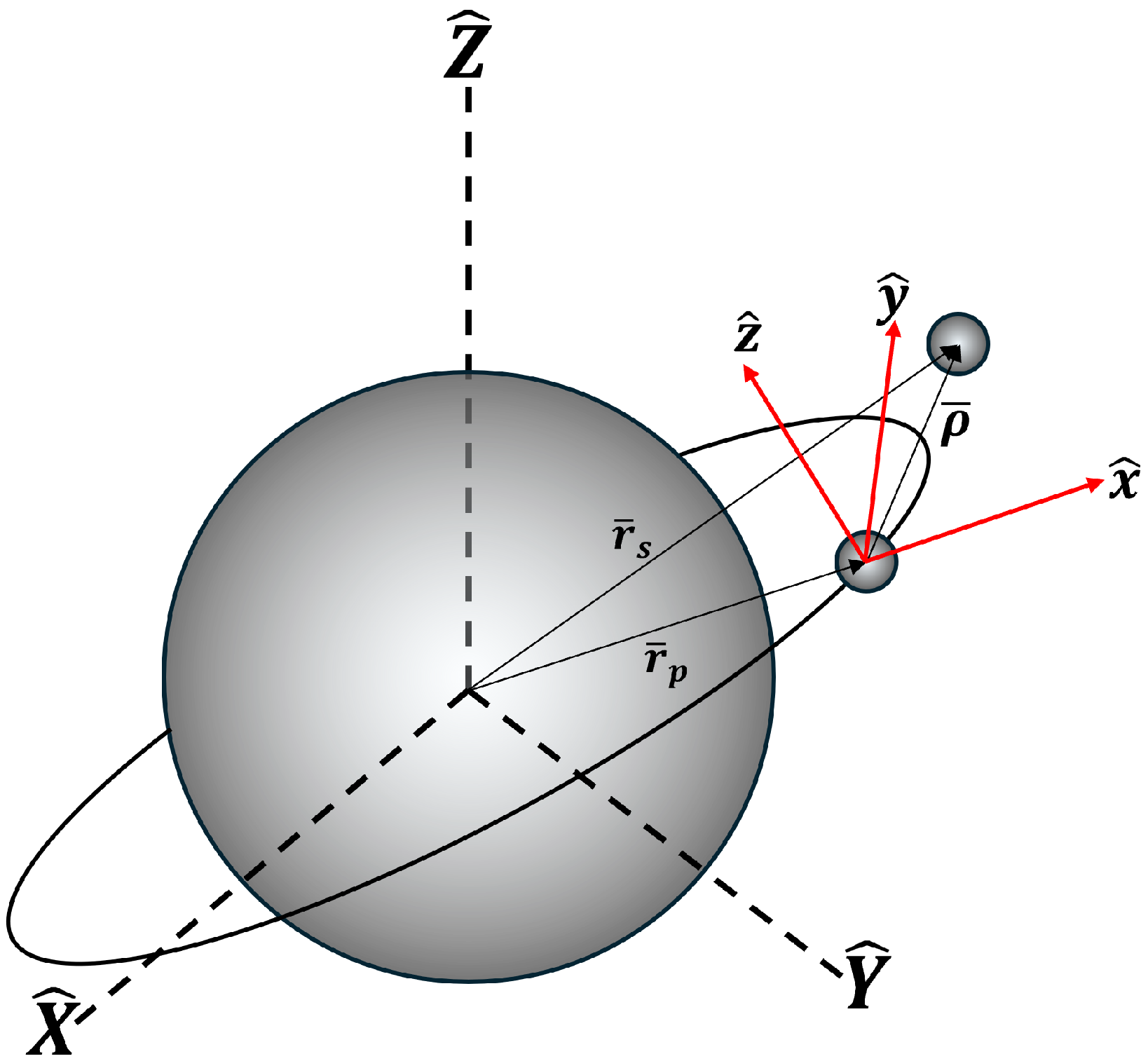
In Figure 1, it can be seen that ${\overline{r}}_p$ and ${\overline{r}}_s$ are the three-element position vectors for the primary and secondary satellites, respectively, with each component of the positions defined as:

$${\overline{r}}_p=X_p\widehat{X}+Y_p\widehat{Y}+Z_p\widehat{Z}$$

$${\overline{r}}_s=X_s\widehat{X}+Y_s\widehat{Y}+Z_s\widehat{Z}$$

Given the positions of the the primary and secondary satellites in the inertial frame, the governing equations of motion (EOMs) accounting for $J_2$ perturbations are defined as:

$$\ddot{\overline{r}}=-{\displaystyle \frac{\mu }{|\overline{r}{|}^3}}\left[\begin{array}{c}X[1-{\displaystyle \frac{3}{2}}{J}_2{\left({\displaystyle \frac{R_e}{|\overline{r}|}}\right)}^2({\displaystyle \frac{5Z^2}{|\overline{r}{|}^2}}-1)]\\ Y[1-{\displaystyle \frac{3}{2}}{J}_2{\left({\displaystyle \frac{R_e}{|\overline{r}|}}\right)}^2({\displaystyle \frac{5Z^2}{|\overline{r}{|}^2}}-1)]\\ Z[1-{\displaystyle \frac{3}{2}}{J}_2{\left({\displaystyle \frac{R_e}{|\overline{r}|}}\right)}^2({\displaystyle \frac{5Z^2}{|\overline{r}{|}^2}}-3)]\end{array}\right]+{\overline{u}}^{\mathcal{I}}$$

(1)

where ${\overline{u}}^{\mathcal{I}}$ is the specific control thrust in inertial components, Earth’s equatorial radius is $R_e=6378$ km, Earth’s gravitational parameter is $\mu =3.986\times {10}^5$ km³/s², the oblateness coefficient $J_2=1.08\times {10}^{-3}$, and the subscript on the coordinates has been removed since the equations are application to both satellites.

The control (i.e., the specific thrust vector on the secondary satellite) is developed using the relative state vector. The relative position vector is expressed in the rotating relative frame $\mathcal{R}$ shown in Figure 1:

$$\overline{\rho }=x\widehat{x}+y\widehat{y}+z\widehat{z}$$

(2)

To construct the $\mathcal{R}$ frame, the origin is centered on the primary satellite, with the radial axis $\widehat{x}$ pointing radially outwards and the cross-track axis $\widehat{z}$ pointing orthogonal to the orbital plane of the primary satellite. The in-track axis $\widehat{y}$ is orthogonal to both the $\widehat{x}$ and $\widehat{z}$ axes to complete the relative frame. To convert the specific thrust from $\mathcal{R}$ to $\mathcal{I}$, the rotation matrix $\mathrm{Z}$ is defined based on the state of the primary in the ECI frame:

$$\mathrm{T}=\left[\begin{array}{c}{\displaystyle \frac{{\overline{r}}_p}{|{\overline{r}}_p|}}\\ \left({\displaystyle \frac{{\overline{r}}_p\times {\overline{v}}_p}{|{\overline{r}}_p\times {\overline{v}}_p|}}\right)\times \left({\displaystyle \frac{{\overline{r}}_p}{|{\overline{r}}_p|}}\right)\\ {\displaystyle \frac{{\overline{r}}_p\times {\overline{v}}_p}{|{\overline{r}}_p\times {\overline{v}}_p|}}\end{array}\right]$$

(3)

where ${\overline{v}}_p$ is the velocity vector of the primary satellite. Given the rotation matrix, the conversion of the specific thrust control from $\mathcal{R}$ to $\mathcal{I}$ is:

$${\overline{u}}^{\mathcal{I}}=\left[\mathrm{T}\right]{\overline{u}}^{\mathcal{R}}$$

(4)

where the control, ${\overline{u}}^{\mathcal{R}}$, is developed in the sections below. Equations (1) and (4) provide the equations of motion in the inertial frame that were implemented to propagate both the primary and secondary satellites forward in time.

2.2. Simulation Parameters

To test the performance of the trajectory control scheme developed within this paper, numerical-based simulations were constructed. The initial state of each test case used standardized parameters, which are presented in

Table 1. Primary satellite’s initial keplerian elements.

${\mathit{a}}_{\mathit{p}}$ [km]	${\mathit{e}}_{\mathit{p}}$	${\mathit{i}}_{\mathit{p}}$[°]	${\mathbf{\Omega }}_{\mathit{p}}$[°]	${\mathit{\omega }}_{\mathit{p}}$[°]	${\mathit{\nu }}_{\mathit{p}}$[°]
7000	0	65	0	0	0

and

Table 2. Secondary satellite’s initial relative state vector for a 1 h period.

x [m]	y [m]	z [m]	$\dot{\mathit{x}}$ [m/s]	$\dot{\mathit{y}}$ [m/s]	$\dot{\mathit{z}}$ [m/s]
0	200	0	0.1745	0	0.3491

below, where $a_p$, $e_p$, $i_p$, ${\mathrm{\Omega }}_p$, ${\omega }_p$ and ${\nu }_p$ are the semi-major axis, eccentricity, inclination, right ascension of the ascending node, argument of perigee, and true anomaly, respectively, of the primary satellite.

An example satellite in low Earth orbit (LEO) is considered with a semi-major axis of 7000 km and 65° of inclination; all other orbital parameters were set to zero. These orbital parameters were all considered osculating elements in the computation of the initial state.

The initial state of the secondary satellite was defined using the relative state as the more natural coordinates for the mission design. To convert these states to the inertial states that are propagated in the nonlinear simulation, the algorithm in Example 14.3 from Ref. [18] is employed. The initial relative states in Table 2 correspond to a one-hour period for the forced motion, a semi-minor axis of the relative in-plane ellipse (i.e., in the plane of the orbit) of 100 m and an out-of-plane amplitude of 200 m, i.e., C = 100 m and D = 200 m in Equation (13) below. The one-hour period of the circumnavigation is 62% of the natural 97 min (5830 s) period.

For most mission scenarios, the relative ellipse size will typically be as small as possible, while minimizing the risk of detection or collision.

2.3. Uncontrolled Motion

The unforced, natural relative motion of the two satellites defined above is discussed in this section for two reasons. First, the unperturbed version of the resulting relative ellipse is used for the baseline relative motion geometry of the faster-than-natural circumnavigation (only the period is changed). Second, the error between the perfect ellipse and the perturbed motion for this uncontrolled case provides some metric with which to compare the performance of the controlled motion.

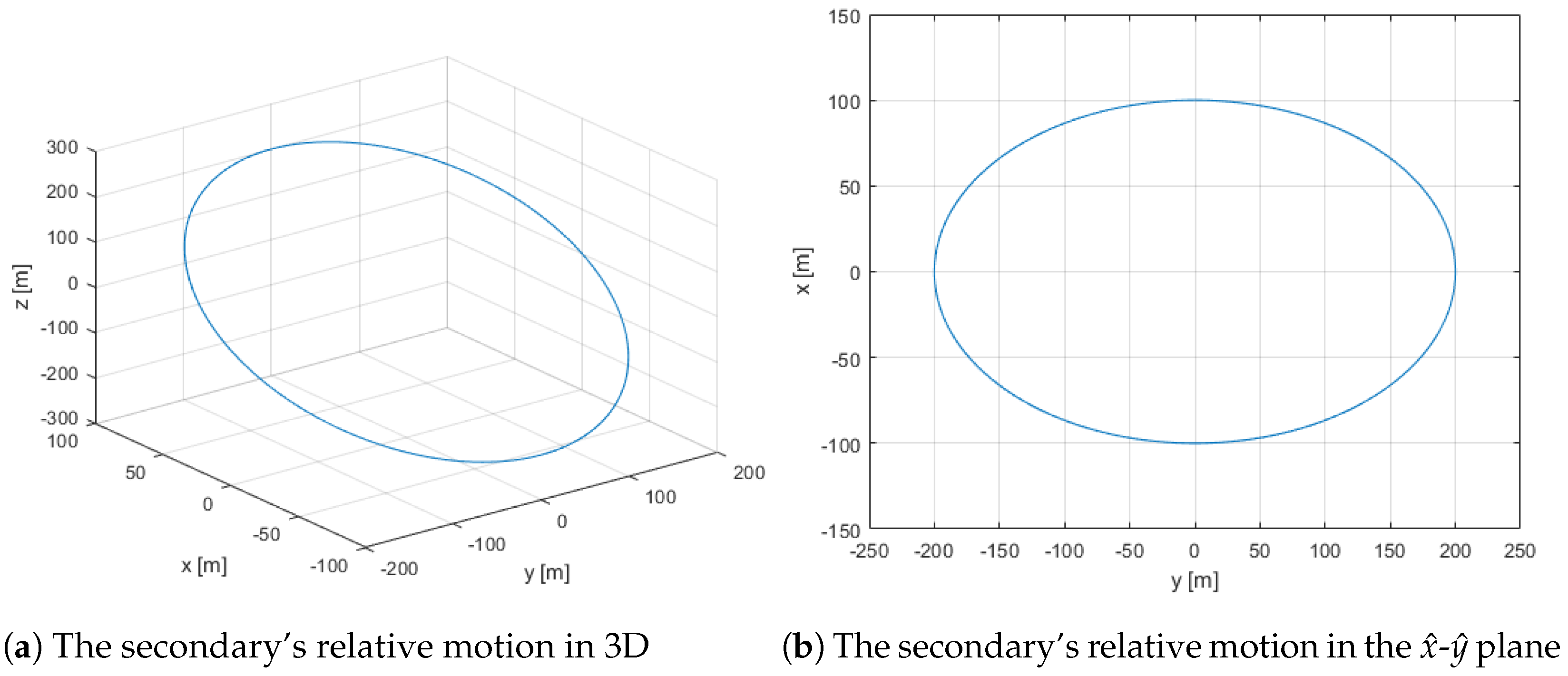
Given these initial conditions, Equation (1) for both the primary and secondary satellites was propagated forward in time. The resulting relative motion seen in Figure 2 of the secondary about the primary exhibits the typical behavior of uncontrolled motion.

In Figure 2b, it can be seen that the relative motion results in a 2 × 1 ellipse on the $\widehat{x}-\widehat{y}$ plane, which is the plane of the orbit. This behavior is a result of the coupled nature of the radial and in-track accelerations. The radial component of the relative motion is subject to simple harmonic motion, while the in-track component comprises both simple harmonic motion as well as linear drift due to a small change in the mean motion of the secondary. A minor discontinuity is present in both graphs at the starting and ending point of the orbit, which is a result of the perturbed motion induced by $J_2$ effects. For this baseline case, the out-of-plane amplitude of 200 m is achieved via a change in the inclination of the absolute orbit of the secondary satellite (versus a change in right ascension of the ascending node). This maximizes the differential perturbation due to $J_2$.

The effect due to $J_2$ perturbations becomes increasingly apparent by extending the propagation of Equation (1) for 5 orbits. The results, shown in Figure 3, demonstrate a linearly increasing amplitude in error residuals between the nominal and propagated states as well as a secular trend in the in-track component. It can be shown that most of this maximum 19 m error between the nonlinear propagation and the perfect ellipse is due to $J_2$, since excluding $J_2$ from the model yields a maximum error of 0.6 m in the in-track direction and less than 50 cm in both radial and cross-track directions. These remaining errors are due to the nonlinearities of the system and integration error.

3. Feedforward Controller

The feedforward control represents the nominal control that is needed to track the nominal faster-than-natural relative path assuming a linear dynamics model with no disturbances. It is the exact (optimal) control for the desired path and the simplified model. It is not necessarily stable or optimal when implemented in a realistic model, but as long as the disturbances are relatively small, then the difference between feedforward and optimal control is also small.

To prove this assertion consider a the linear system:

$$\dot{\overline{x}}=A\overline{x}+{\overline{u}}^{\mathcal{R}}$$

(5)

Assume the feedforward control ${\overline{u}}_{FF}^{\mathcal{R}}\left(t\right)$ exactly yields the solution ${\overline{x}}_{nom}\left(t\right)$, so:

$${\dot{\overline{x}}}_{nom}=A{\overline{x}}_{nom}+{\overline{u}}_{FF}^{\mathcal{R}}$$

(6)

For the actual system with nonlinear terms and disturbances represented by the small general nonlinear term ${\overline{f}}_{ϵ}\left(\overline{x}\right)$, the governing equations are:

$$\dot{\overline{x}}=A\overline{x}+{\overline{f}}_{ϵ}\left(\overline{x}\right)+{\overline{u}}^{\mathcal{R}}$$

(7)

Assume control ${\overline{u}}^{\mathcal{R}}={\overline{u}}_{FF}^{\mathcal{R}}+\delta {\overline{u}}^{\mathcal{R}}$ results in the same nominal motion for the actual system. Performing some simple algebra using Equation (6) demonstrates that the deviation from the nominal control (i.e., the difference between the feedforward control and the perfect optimal control) is equivalent to the small unmodelled nonlineaarities and disturbances:

$$\delta {\overline{u}}^{\mathcal{R}}={\overline{f}}_{ϵ}\left(\overline{x}\right)$$

(8)

This result is the fundamental justification for the feedforward controller. Since the feedforward control provides all but some small deviation from the desired control, the feedback control gains needed to account for unmodelled effects can be small. This in turn results in lower control effort and less sensitivity to noise than a controller that uses only feedback control.

To compute the feedforward control, the linearized relative equations of motion as defined by Clohessy and Wiltshire [19] are used:

$$\begin{array}{c}\hfill \ddot{x}-2n\dot{y}-3n^{2}x=u_x\end{array}$$

(9a)

$$\begin{array}{c}\hfill \ddot{y}+2n\dot{x}=u_y\end{array}$$

(9b)

$$\begin{array}{c}\hfill \ddot{z}+n^{2}z=u_z\end{array}$$

(9c)

where n is the mean motion of the primary satellite (i.e., the reference trajectory) and $u_x$$,u_y$, and $u_z$ are components of the specific thrust vector, ${\overline{u}}^{\mathcal{R}}$. The well-known solution to the natural (${\overline{u}}^{\mathcal{R}}=\overline{0}$) motion of the linear equations above for a general closed path (i.e., for equal period of the primary and secondary satellites) is:

$$\begin{array}{c}\hfill x\left(t\right)=Csin(nt-\alpha )\end{array}$$

(10a)

$$\begin{array}{c}\hfill y\left(t\right)=2Ccos(nt-\alpha )+y_{off}\end{array}$$

(10b)

$$\begin{array}{c}\hfill z\left(t\right)=Dsin(nt-\beta )\end{array}$$

(10c)

where C is the semi-minor axis of the projected relative ellipse into the orbital plane, D is the out-of-plane amplitude, $\alpha$ is the phase angle for the in-plane motion, $\beta$ is the phase angle for out-of-plane motion and $y_{off}$ is the offset of the center of the relative ellipse in the alongtrack direction.

This natural motion solution is used to specify the geometry of the nominal relative motion (i.e., the path irrespective of time). To achieve a faster-than-natural baseline trajectory, we simple change the angular velocity from the mean motion of the primary to some specified, $\dot{\theta }$, which determined by the desired relative orbital period ${\mathrm{P}}_{rel}$:

$$\dot{\theta }={\displaystyle \frac{2\pi }{{\mathrm{P}}_{rel}}}$$

(11)

Thus, the set of equations used to define the nominal position of the secondary satellite on a faster-than-natural circumnavigation trajectory at any given point in time is given as:

$$\begin{array}{c}\hfill x\left(t\right)=Csin(\dot{\theta }t-\alpha )\end{array}$$

(12a)

$$\begin{array}{c}\hfill y\left(t\right)=2Ccos(\dot{\theta }t-\alpha )+y_{off}\end{array}$$

(12b)

$$\begin{array}{c}\hfill z\left(t\right)=Dsin(\dot{\theta }t-\beta )\end{array}$$

(12c)

All of the error plots in the sections below are with respect to nominal motion given by Equation (12).

To determine the feedforward control for the nominal motion of Equation (12), the first and second time derivatives of Equation (12) are determined and substituted into Equation (9). The resulting expressions for the feedforward control are:

$$\begin{array}{c}\hfill u_x=-Csin\left(\dot{\theta }t\right)({\dot{\theta }}^2+4n\dot{\theta }+3n^2)\end{array}$$

(13a)

$$\begin{array}{c}\hfill u_y=-2C\dot{\theta }cos\left(\dot{\theta }t\right)(\dot{\theta }-2n)\end{array}$$

(13b)

$$\begin{array}{c}\hfill u_z=-Dsin\left(\dot{\theta }t\right)({\dot{\theta }}^2-n^2)\end{array}$$

(13c)

These relative frame components make up the ${\overline{u}}^{\mathcal{R}}$ vector of Equation (4) for the simulation results of this section and will more specifically be referred to as the feedforward control ${\overline{u}}_{FF}^{\mathcal{R}}$ in later sections. Note that the feedforward control is proportional to the size of the ellipse. For fast circumnavigates where $\dot{\theta }$ is much larger than the mean motion, the control is proportional to the square of the relative angular velocity, i.e., inversely proportional to the square of the relative period.

To assess the performance of this feedforward control scheme, a sample mission was simulated based on the specifications outlined in Section 2.2. The control is implemented in the nonlinear simulation as a zero-order hold, where the continuous thrust value is updated at a 1 Hz frequency. A scenario was tested with a relative orbital period of 1 h and a relative ellipse geometry given by $C=$100 m, $D=$ 200 m, and $\alpha =\beta =0$. 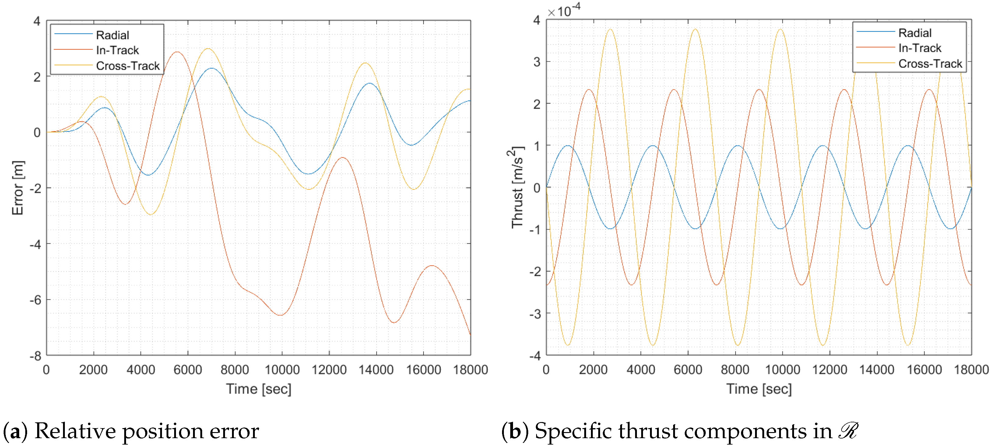The results, propagated over five relative orbits, are shown in Figure 4.

Figure 4a shows the deviation between nominal and propagated relative orbits in component form, with Figure 4b illustrating the components of the feedforward thrust as derived from Equation (13). The primary source of the error seen in Figure 4a is the zero-order hold, which causes a delay in thrust updates. This delay results in a discrepancy between the necessary and actual thrust at each moment in time. Since the feedforward control does not utilize real-time relative state feedback, the controller cannot adjust itself to reduce the error, leading to an uncorrected drift that compounds over time. Consequently, the system’s performance is heavily dependent on accurate pre-calculated trajectories and thrust commands. Any unmodeled perturbations will increase the deviation, as the controller lacks the capacity to correct for unforeseen disturbances or errors. The effect of unmodeled perturbations can be seen in Figure 4, as $J_2$ perturbations are not included in the computation of the thrust. This adds to the already compounding error of the feedforward control architecture. This limitation drives the need for a feedback mechanism to achieve better precision in maintaining the desired relative orbit.

The maximum magnitude of the control effort in Figure 4b is $4.0\times {10}^{-4}$ m/s², which is larger by about a factor of two compared to a capable current-day continuous-thrust spacecraft [20,21]. For example, Ref. [21] cites a maximum acceleration of $2.3\times {10}^{-4}$ m/s² for the SpaceX (Hawthorne, CA, USA) Starlink V2.0 mini satellite. However, none of the spacecrafts surveyed were optimized for this particular mission, since no such satellite has been acknowledged in the open literature. So, the levels of thrust dictated here are likely to be possible in an optimized spacecraft design with current or very near-term technology. As discussed below, for relative orbits smaller than the baseline of this work, the thrust requirements can be significantly reduced. Thus, advances in relative navigation, which can reduce the required distance to maintain safety, can also improve the practicality of this mission concept.

4. Feedback Control with a Linear Quadratic Tracker

The implementation of a feedback controller reduces the errors caused by disturbances that are not accounted for in the feedforward model. The feedback controller presented is a modified linear quadratic regulator, which is implemented such that the control drives the error between the nominal state and the simulated state to zero; this premise is herein referred to as linear quadratic tracking (LQT). This LQT method begins by defining the cost function, J:

$$J={\displaystyle \frac{1}{2}}{\int }_0^{t_f}({\overline{e}}^{T}Q\overline{e}+{\left({\overline{u}}^{\mathcal{R}}\right)}^{T}R{\overline{u}}^{\mathcal{R}})dt$$

(14)

where $\overline{e}$ is the relative state error between the nominal and actual trajectories and Q & R are the state and control weight matrices, respectively. Both weighting matrices must be symmetric and positive definite in order for the following formulations to be valid.

Assume the relative dynamics are represented by the linear system:

$$\dot{\overline{x}}=A\overline{x}+B{\overline{u}}^{\mathcal{R}}$$

(15)

Then, the optimal solution to Equation (14) is:

$${\overline{u}}^{\mathcal{R}}={\overline{u}}_{FB}^{\mathcal{R}}=-R^{-1}{B}^{T}S\left(t\right)\overline{e}\left(t\right)$$

(16)

where we have used the subscript $FB$ to distinguish this feedback control from the feedforward control, S represents the control gain matrix, and matrix B is a 6 × 3 control input matrix defined as:

$$B=\left[\begin{array}{ccc}0& 0& 0\\ 0& 0& 0\\ 0& 0& 0\\ 1& 0& 0\\ 0& 1& 0\\ 0& 0& 1\end{array}\right]$$

To obtain an expression for the control gain matrix, the infinite-horizon algebraic Riccati equation is used:

$$0=SA+A^{T}A-AB{R}^{-1}{B}^{T}S+Q$$

(17)

where the matrix A is a 6 × 6 matrix of constant coefficients derived from the Clohessy-Wiltshire equations presented in Section 3.

$$A=\left[\begin{array}{cccccc}0& 0& 0& 1& 0& 0\\ 0& 0& 0& 0& 1& 0\\ 0& 0& 0& 0& 0& 1\\ 3n^2& 0& 0& 0& 2n& 0\\ 0& 0& 0& -2n& 0& 0\\ 0& 0& -n^2& 0& 0& 0\end{array}\right]$$

Equation (17) was solved using the ‘lqr’ function in MATLAB (R2022b) to yield a constant gain matrix, S. It is worth noting that the finite-horizon Riccati is an equally viable solution path, but analysis showed that there was no appreciable increase in performance. The resulting expression for the optimal thrust given in Equation (16) is subsequently transformed from the $\mathcal{R}$ frame to $\mathcal{I}$ and is applied to the non-linear equations of motion defined in Equation (1).

To define a reasonable error bound for the controller tuning, we reference the study by Zhang et al., which quantifies the measurement accuracy of various techniques. Their findings indicate that when utilizing electro-optical and radio frequency sensors, the combined measurement accuracy typically achieves approximately 10 cm for a relative separation distance of 100 m [22]. To accommodate potential off-nominal situations, we extend this measurement accuracy by a multiple of 5, resulting in a maximum error bound of 50 cm for the feedback architecture. This error bound serves as the design requirement for the controller, which is achieved by adjusting the Q and R matrices. Equal weights are assumed for all states in the Q matrix and the control components in the R matrix. Since the cost function only depends on the ratio of the Q and R matrices, this leaves only one scalar variable to be tuned. The scalar multiplier for the R matrix is determined iteratively in order to satisfy the constraint on the error bound. For the baseline case this yields:

$$\begin{array}{ccc}\hfill Q=I_{6\times 6}& \hfill & \hfill R=1.5\times {10}^6\left[I_{3\times 3}\right]\end{array}$$

where $I_{n\times n}$ is an n × n identity matrix. The resulting gain matrix needed to accurately track the relative trajectory only through feedback on state errors is quite large and therefore susceptible to noise as described below. This is the main weakness of using feedback control for faster-than-natural motion.

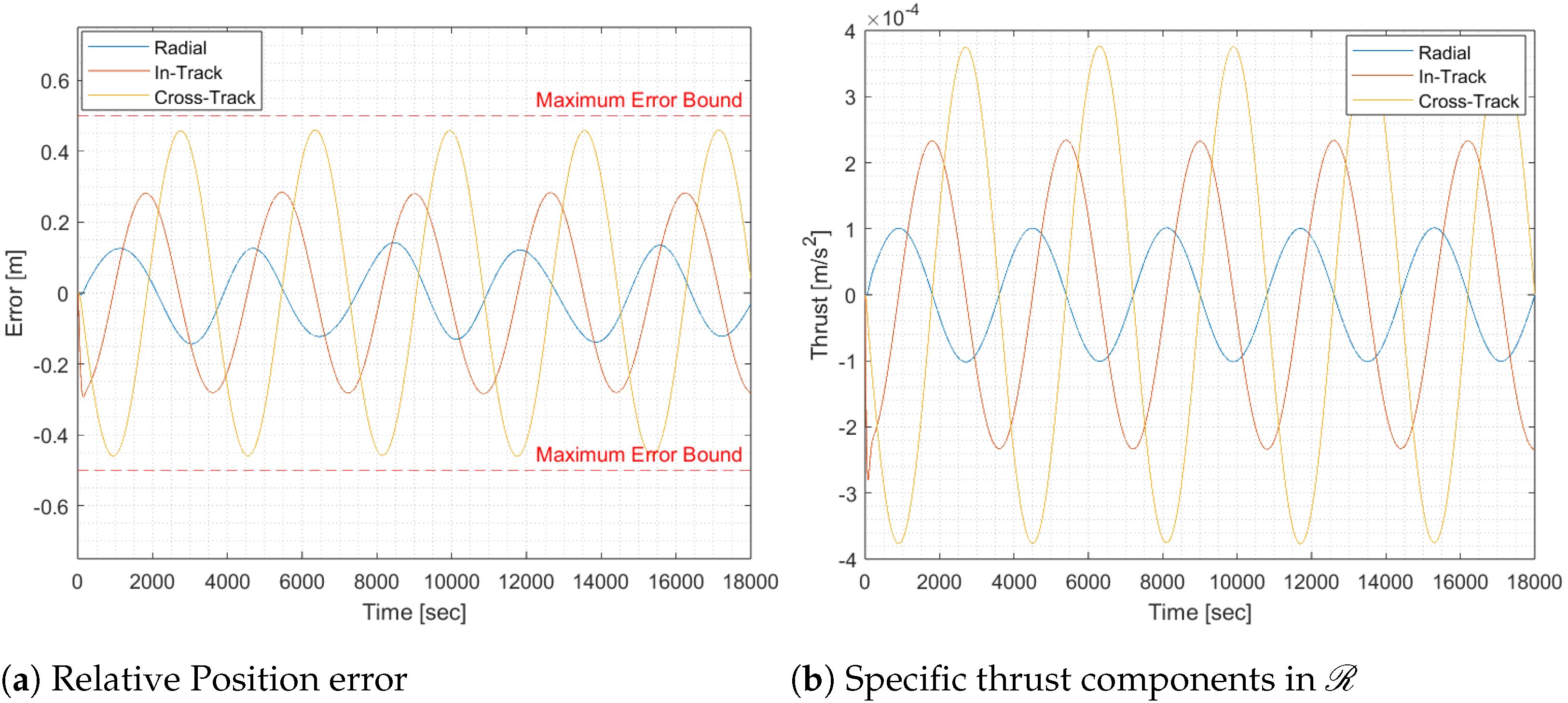
To evaluate the performance differences between feedforward and feedback architectures, we conducted the simulated mission based on the parameters specified in Section 2.2 in conjunction with the desired relative period of 1 h. The resulting error and thrust components for the feedback control architecture, propagated over five relative orbits, are illustrated in Figure 5.

When comparing the feedback thrust in Figure 5b to the feedforward thrust in Figure 4b, the difference in control is negligible. However, the relative state error demonstrates significant improvement, with a maximum error of approximately 70 m in the feedforward control compared to just 50 cm with feedback control. Assuming no unforeseen circumstances arise, the periodicity of the error resulting from the feedback controller indicates that the control architecture will maintain the error within the specified 50 cm bound indefinitely. A notable drawback of the feedback control system, however, is its poor transient response, as seen in the beginning of the plot shown in Figure 5b. The transient response overshoots the required steady-state thrust by approximately 4.4%. This overshoot can compound over successive missions, which is particularly undesirable behavior given the fuel limitations on board the satellite.

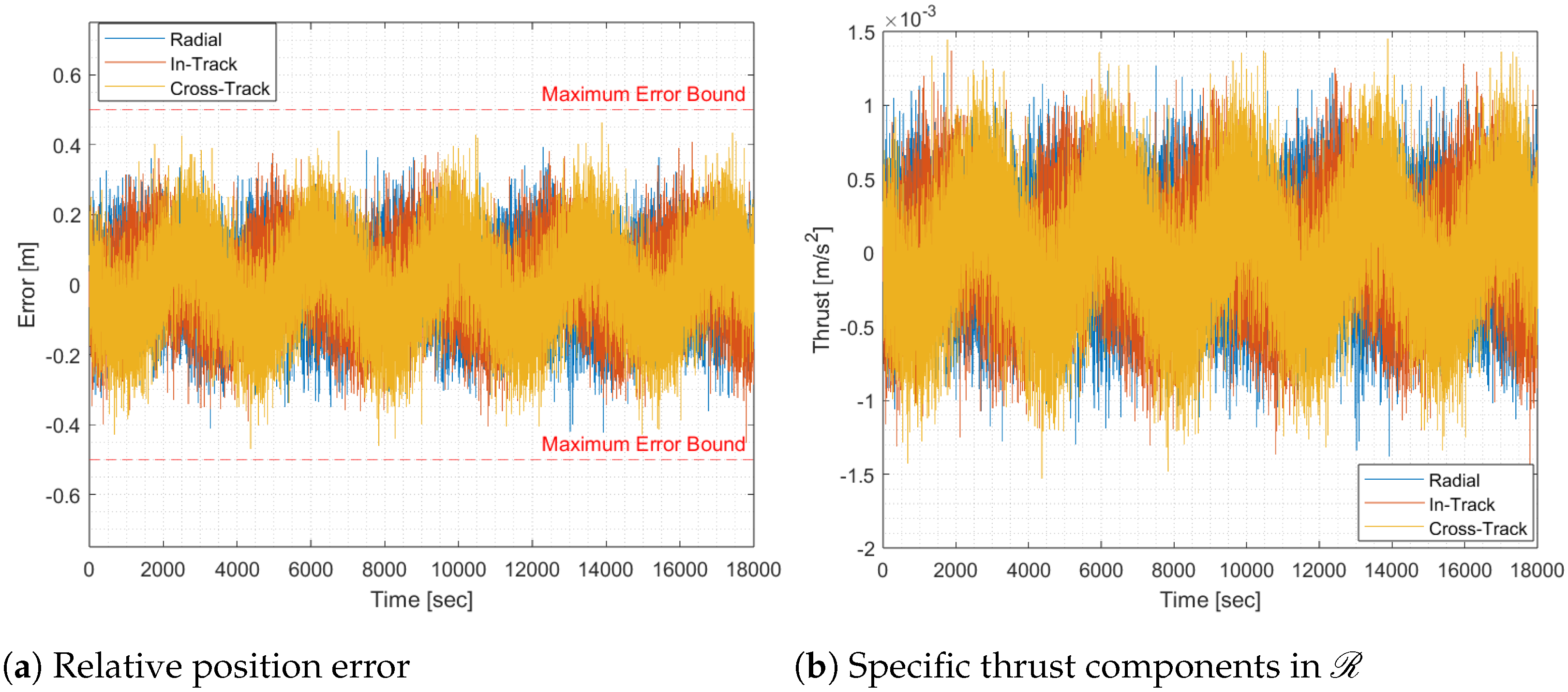
As previously noted, this control architecture is sensitive to noise, which necessitates significantly more thrust to achieve results comparable to the noiseless case presented in Figure 5. In the simulation, noise was introduced as white Gaussian noise (WGN) by generating random scalars from a normal distribution, with a standard deviation of 10 cm for the relative position vector and 0.1 ${\displaystyle \frac{\mathrm{cm}}{\mathrm{s}}}$ for the relative velocity. The WGN was applied to the feedback control at each update to the zero-order hold thrust, resulting in the plots shown in Figure 6. This noise implementation method is designed to offer a low-fidelity approximation of system performance under noisy conditions, though it may not fully capture the noise characteristics of a real-world system. The Q and R matrices required to maintain the maximum error within this bound were defined as:

$$\begin{array}{ccc}\hfill Q=I_{6\times 6}& \hfill & \hfill R=1\times {10}^5\left[I_{3\times 3}\right]\end{array}$$

The introduction of noise causes a thrust increase by more than a factor of two, as illustrated in Figure 6b, when compared to the noiseless thrust in Figure 5b. While the 50 cm error bound remains lower than in the feedforward case, this advantage is outweighed by the higher thrust required to achieve it. The system’s sensitivity to noise reduces robustness, increases fuel consumption, and imposes excessive stress on the actuation of the secondary satellite. These limitations of the feedback control under noisy conditions highlight the need for a combined control architecture, which offers an effective solution for mitigating noise.

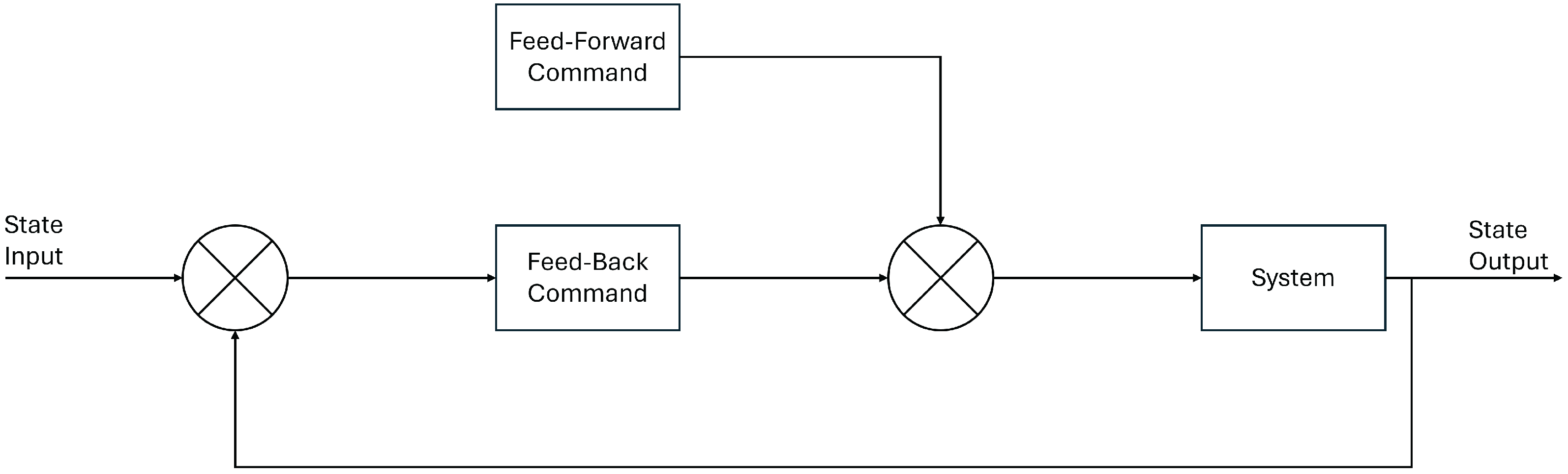
5. Combined Control Architecture

A strictly feedforward controller performs poorly in the presence of disturbance while a strictly feedback controller causes the system to be susceptible to noise. The advantages of both of these controllers can be realized through simple superposition:

$${\overline{u}}_{CC}^{\mathcal{R}}={\overline{u}}_{FF}^{\mathcal{R}}+{\overline{u}}_{FB}^{\mathcal{R}}$$

(18)

where the combined control ${\overline{u}}_{CC}^{\mathcal{R}}$ is computed using the feedforward control ${\overline{u}}_{FF}^{\mathcal{R}}$ given by Equation (9) and the feedback control ${\overline{u}}_{FB}^{\mathcal{R}}$ given by Equation (16). Figure 7 below provides a visualization of the final control architecture.

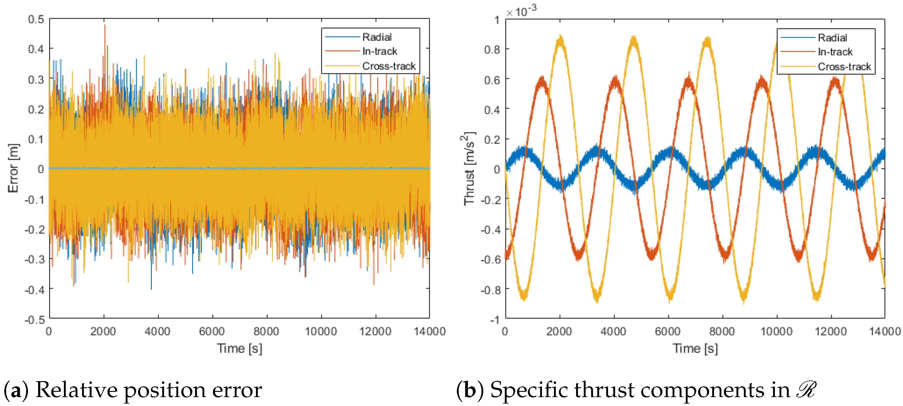
The feedforward control constitutes the vast majority of the thrust, relying on the accuracy of the dynamics model. This allows the feedback component to correct errors caused by perturbations, navigational inaccuracies, and zero-order hold effects. Although the combined architecture is simple in design, its implementation in the simulation leads to a significant improvement in the thrust profile. As in the feedback simulation, a 50 cm error bound was imposed on the controller. The Q and R matrices used to achieve this are:

$$\begin{array}{ccc}\hfill Q=I_{6\times 6}& \hfill & \hfill R=4.5\times {10}^8\left[I_{3\times 3}\right]\end{array}$$

The addition of the feedforward control architecture allows for a much larger weight on the control term of the cost function, which reduces the optimal feedback gains significantly. With these smaller feedback gains, the system becomes less sensitive to noise, and the feedforward term provides the majority of the control needed to accurately track the desired relative trajectory. The simulation results demonstrate the good tracking performance in Figure 8a. The combination of the feedforward and feedback control shown in Figure 8b also reduces the thrust by about one half when compared to Figure 6b and results in a noticeably smoother thrust profile. This smoother thrust profile minimizes the wear on critical hardware components such as actuators and reaction wheels, therefore extending the effective lifetime of the spacecraft. Additionally, since the increase in performance does not result in an appreciable increase in control, this architecture is achievable with current-day low-thrust devices similarly to the feedforward architecture.

To see how the final control performs with a different sized relative ellipse, the values of C and D were halved from 100 m to 50 m while keeping the period the same (1 h) and the feedback gains the same as the baseline. The results are shown in Figure 9. The control effort is reduced for this case since a reduced relative velocity and acceleration are needed to traverse a shorter path in the same amount of time. From Equation (13), there is a linear relationship between the relative orbit size, given by C, and the feedforward control. This is confirmed by the reduction in the control by a factor of two when compared with Figure 8. The control for this case appears slightly noisier than the baseline case because the noise levels are a larger percentage of the states.

The results for a decrease in the relative orbit period to 45 min are shown in Figure 10. The control effort is increased due to the increase in relative velocity and acceleration needed to affect the faster motion. As the angular velocity of the relative motion is increased, the ${\dot{\theta }}^2$ terms dominate the terms containing the mean motion, n, in Equation (13). Thus, the increase in the relative angular velocity by a factor of ${\displaystyle \frac{4}{3}}$ for this case causes about a ${\left({\displaystyle \frac{4}{3}}\right)}^2=1.8$ factor increase in the control as evident when comparing Figure 8 and Figure 10.

This controller is also applicable to other orbital regimes. As described for the relative angular velocity increase, the terms containing n become negligible as the absolute orbit radius increase and the control becomes nearly invariant with respect to altitude. Thus, the results for larger orbits are very similar to the LEO case. The results for different orbital planes are also very similar to the baseline since the differential motion due to oblateness is relatively small and easily removed with the feedback control. Variations in the size of the relative baseline motion exhibit the same type of behavior shown in the examples above, with the salient feature that the control effort decreases with decreased path length of the relative ellipse.

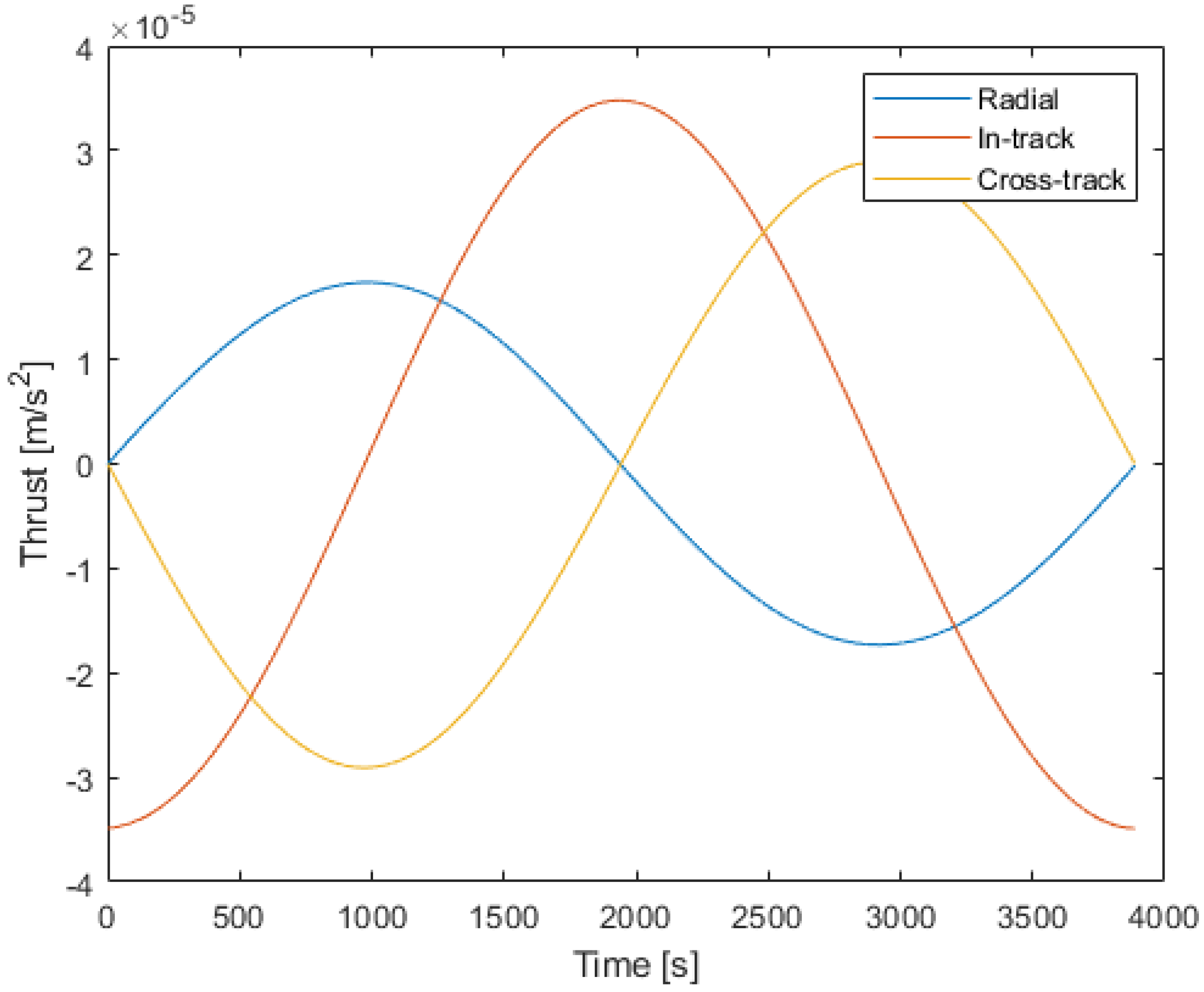
The control effort can be quantified in a single metric by integrating the absolute value of the specific thrust magnitude to get a total $\Delta V$ for the circumnavigation. For the baseline case, using a simple rectangle integration approximation yields a total $\Delta V$ of 1.038 m/s for one period of the relative trajectory. Using this metric, the control effort of the continuous control can be compared to the results for impulsive control from Ref. [12]. In Figure 5 of Ref. [12], the $\Delta V$ requirements are given for circumnavigation at different distances from the primary satellite with different relative motion periods. For the case with a radial distance of 20 meters, an alongtrack distance of 40 m, an out-of-plane distance of 20 m, and a relative frequency of 1.5 times the mean motion of the primary, the $\Delta V$ from Ref. [12] is about 0.1 m/s. Implementing the continuous control of this paper for the equivalent case (C = D = 20 m and $\dot{\theta }=1.5n$) for the period of 3886 s yields the control given in Figure 11. The computed $\Delta V$ for this continuous control is 0.12 m/s. While this is larger than the impulsive case, the specific impulse advantage of the continuous thrust system would typically result in a significantly lower propellant mass.

6. Conclusions

This paper demonstrates that continuous control for faster-than-natural satellite circumnavigation is a practical mission design option. A specific control architecture is proposed consisting of a newly developed feedforward controller that is used in conjunction with an existing feedback control scheme. The feedforward term constitutes the majority of the control needed to track the desired relative motion, allowing for reduced gains on the feedback control, which avoids excessive control effort and sensitivity to noise. The architecture offers an intuitive solution, yet its effectiveness cannot be overstated, as it strikes an essential balance between robustness and efficiency in control effort. For cases where increased performance is required, the feedforward component of the control can be refined to account for additional dynamics such as oblateness or differential drag.

Future Work

The findings in this paper open several avenues for advancing the validity of the control algorithms discussed. Firstly, these algorithms currently do not account for the attitude dynamics of the secondary satellite. This limitation could become critical if the satellite lacks gimbal-mounted equipment, such as sensors or antennas, as misaligned thrusts could impact mission objectives. Future work should focus on incorporating attitude control into the algorithm, ensuring precise alignment of thrust and payload orientation while allowing the on-board sensors to collect observation data of the primary satellite. To ensure that each thruster achieves the desired thrust vector, advanced thruster actuation methods should be developed, enabling precise control over the combined thrust output in alignment with the requirements of the control algorithm. Additionally, the current approach to noise modeling within the feedback and combined control architectures may not fully reflect the complexities of a physical system. To improve the accuracy of the noise representation, future work should integrate more comprehensive models, including detailed sensor systems and measurement filters, that capture realistic system noise. This enhancement will contribute to more robust simulations that better predict real-world performance.