Article

Observer for Nonlinear Systems with Time-Varying Delays: Application to a Two-Degrees-of-Freedom Helicopter

by
Omar Hernández-González
1,
Felipe Ramírez-Rasgado
2,3,
Mondher Farza
3,
María-Eusebia Guerrero-Sánchez
4,*,
Carlos-Manuel Astorga-Zaragoza
2,
Mohammed M’Saad
3 and
Guillermo Valencia-Palomo
1
1
Tecnológico Nacional de México, IT Hermosillo, Av. Tec. 115, Hermosillo 83170, Mexico
2
Tecnológico Nacional de México, Centro Nacional de Investigación y Desarrollo Tecnológico, Internado Palmira S/N, Col. Palmira, Cuernavaca 62490, Mexico
3
Laboratoire d’Ingénierie des Systèmes (LIS, UR7478, Université de Caen Normandie, École Nationale Supérieure d’Ingénieurs de Caen), 6 Bd. Maréchal Juin, 14050 Caen, France
4
CONAHCyT-Tecnológico Nacional de México, IT Hermosillo, Av. Tec. 115, Hermosillo 83170, Mexico
*
Author to whom correspondence should be addressed.
Aerospace 2024, 11(3), 206; https://doi.org/10.3390/aerospace11030206
Submission received: 18 January 2024 / Revised: 2 March 2024 / Accepted: 4 March 2024 / Published: 6 March 2024

Abstract

:
This paper deals with the problem of the estimation of non-uniformly nonlinear systems with time-varying delays in the state and input. In addition, the problem of the sampled output measurement is also been addressed. Thus, an observer design for a class of uncertain, non-uniformly nonlinear systems in the presence of time-varying delay is proposed. A continuous–discrete observer based on a high-gain approach is designed to achieve undelayed estimation. Thus, sufficient conditions to ensure the convergence of the observer are obtained. The analysis is based on a Lyapunov–Krasovskii functional, which shows that the bounded observation error depends on the sizes of the known upper delay and the upper sampling rate. The performance of the proposed algorithm is evaluated by considering a control-based observer for a two-degrees-of-freedom helicopter system with a known time-varying delay and sampled output measurements.

1. Introduction

In recent years, control theory has focused its efforts on solving problems related to system delays [1,2,3,4,5,6,7,8,9]. Time delays can originate from various sources, including but not limited to communication networks, unmodeled inertia, inherent delays induced by sensors, and communication overhead, among others. On the other hand, in many applications, the knowledge of the state vector is necessary for monitoring and control. Recent works considering state estimation for systems with a known time delay are shown in [10,11,12]. Different authors have addressed the observer design for linear systems. For instance, a Luenberger-like observer is proposed in [13] to estimate the state vector for a system with a known time-varying delay affecting the output. Based on the H approach, an observer is proposed in [14]. An extended state observer for continuous and discrete systems is proposed in [15], considering that the input and the states are time-delayed. For nonlinear systems, different approaches have been presented to reconstruct the state vector of the system, making the error converge to zero if there are no uncertainties in the system or to a region close to the origin; some works on these systems are presented in [6,16,17].
The challenge of designing observers for systems with delays is that delays can vary over time, affecting the system’s performance, and, therefore, the observer has to be able to follow these dynamics. Some works that address these designs considering uncertain but bounded delay functions are presented in [18,19,20,21,22]. In [18], an adaptive observer is proposed, which is designed with the maximum delay present in the system, where the error convergence to zero is only ensured when the delay in the system is equal to the delay in the observer. An extension of this work for a more general class of systems is presented in [19]. For instance, a Luenberguer-like observer is designed in [21], where the observer gain is obtained by linear matrix inequalities (LMIs). For the case where a time delay is present in the output signal, cascade structures have been proposed to reconstruct the current state vector [22,23]. In [22], the actual vector can be estimated using a cascade observer with an error equal to the difference between the actual delay and the set in the observer. An observer-based sliding mode is proposed in the base, and the predictors are of a traditional structure. It is important to emphasize that in the works mentioned above, it is possible to establish that the observation error will converge to a region near the origin since there will be an error between the delay value with which the observer is designed and the actual value presented by the system. Other design techniques have also been proposed by considering the H and Linear Parameter Varying (LPV) approaches to relax the imposed conditions. An observer is designed in [24], where the state and output of the system are affected by a bounded time-varying unknown delay.
However, it is often possible to know the delay functions or to characterize them, which makes it possible to avoid errors between the real system and the observer; for control actions, this estimation is not useful as it has large correction terms. Some works dealing with the design of observers for known variant delays are shown in [5,25,26,27,28,29]. In [25], an observer is proposed for a non-linear system with state delays. The observer has two behavior modes: when it is sampled and when it is not sampled. When the sample is present, the error is obtained by considering the difference between the real output and the estimated output. When the sample is not present, it behaves as a predictor. In this case, the stability of the observer is achieved by calculating a series of LMIs that depend on the value of the delay and the sampling time.
For discrete nonlinear systems with delayed states and unknown inputs, an observer is presented in [26]. The observer is designed by first transforming the nonlinear system to reconstruct the unknown signal with the knowledge of the available states, then transforming it to a Takagi–Sugeno representation, which achieves its nonlinear representation but with the possibility to use techniques for linear systems. The observer gain is obtained by solving LMIs; the main disadvantage of this approach is the number of LMIs that have to be satisfied at once to find the global solution of the system and some matrix properties in the system transformation. One way to relax the solution of LMIs is to consider only the performance of the system at certain values, which gives rise to the design of one-sided-Lipschitz observers, as shown in [27,29]. In [27], the design of an observer is proposed for a descriptor system with delays in the states and the output, but with the assumption that it is possible to measure delay and delay-free signals, as well as uncertainties and disturbances. The main advantage of this system over the others is that it limits the system to work only in one region, and with this, it is possible to consider one side of Lipschitz, relaxing the calculation of the LMIs. The observer is designed to consider robustness margins to achieve convergence in the presence of uncertainties and disturbances. An approach that seeks to reduce the number of estimated states is presented in [29], where a reduced-order observer design for nonlinear systems considering input and output delays is presented. The particularity here is that it does not estimate the whole state vector but only the states that are not available.
Another interesting approach, based on using predictors, is shown in [5]. This paper presents an observer of an uncertain nonlinear system whose control signal is delay-invariant. An extended state observer is proposed for the estimation, allowing for the simultaneous estimation of the state vector and the uncertain function. The observer’s structure adopts a cascade configuration, which is estimated by subsystems in an interval of the delay value and compensates for the variations of the delay present in the input using the Newton–Leibniz formula. The observer gain is obtained by solving an LMI encompassing the original system and the predictors. In [28], an observer is proposed for a class of switched discrete nonlinear systems. Depending on the signal, it switches between different types of systems. The particularity is that it considers delays in the state vector and uncertain parameters in each system. Observer-based control is achieved using a predictive control with a finite time horizon.
The main contribution of this work is that it presents an observer that can reconstruct the current state vector continuously for an uncertain nonlinear system whose outputs are only available in time instants and have delays. Likewise, the delay is present in the dynamics of the system. Most of the above works assume that output measurements are available in continuous time. However, this assumption is restrictive in real-world applications because of the limited hardware capabilities. This work presents the synthesis of a high-gain continuous–discrete observer for a wider class of nonlinear, non-uniformly observable systems compared to that shown in [18,21,30,31]. This class of systems is introduced in Section 2. For this class of systems, the observability properties are satisfied via a persistent excitation condition, as in [32]. Section 3 presents the proposed observer under variable time delay. Its stability is ensured by a Lyapunov–Krasovskii functional, which ensures that the error converges to a bounded region near zero due to the uncertainties, and the convergence rate depends on the sampling in the system. The observer synthesis considers a significant improvement compared to the observer presented by [18,30,31,33]. The improvement is to propose an observer structure that can continuously reconstruct the system state vector in the presence of measurements acquired in time intervals since the authors do not consider this case. In practice, it is a common situation. Likewise, an extension is made for the case where there are multiple outputs and not being limited to one. Another main differentiator is that, in this case, the observer can deal with delays in the output, which, in control systems, due to latency or delays inherent in the communication networks, are present. To validate this problem, it is proposed to regulate the angular position of a two-degrees-of-freedom helicopter system, where there are samples in the output signal and delays in the input and outputs; this is shown in Section 4. The results showing the effectiveness of the observer-based control are shown in Section 5, where different sampling intervals and time-delay scenarios are tested. Finally, conclusions of the work are presented in Section 6.

2. Problem Statement

Consider the following class of delayed nonlinear systems with sampled and delayed outputs:
SYS : x ˙ = A ( u , x ) x + φ ( x , x τ ( t ) , u , u τ ( t ) ) + B ε ( t ) y τ ( t k ) = C x ( t k τ ( t k ) ) = x 1 ( t k τ ( t k ) )
where x = x 1 , x 2 , , x q T with x τ ( t ) = x τ ( t ) 1 , x τ ( t ) 2 , , x τ ( t ) q T and x k R n k k = 1 q n k = n ; and
A ( u , x ) = 0 A 1 ( u , x 1 ) 0 0 A ( q 1 ) ( u , x 1 , , x ( q 1 ) ) 0 0 0 0
φ ( x , x τ ( t ) ) = φ 1 ( x 1 , x 1 τ ( t ) , u , u τ ( t ) ) φ n ( x , x τ ( t ) , u , u τ ( t ) ) , B = 0 n 1 0 n 1 I n 1 T
C = I n 1 × n 1 0 n 1 × n 2 0 n 1 × n q .
where the current state x R n and each A k ( x ) = A ( x 1 , , x k ) , k = 1 , , q 1 , φ ( u , x ) is a triangular nonlinear vector function with respect to x; the unknown function that denotes model uncertainties is given by ε : [ τ * , + [ R p and is bounded; y τ ( t k ) R p , with p = n 1 , is the sampled and delayed system output; the sampling rate is such that 0 t 0 < < Δ k = t k + 1 t k ; lim k t k = + , and there exists 0 < Δ m Δ M < + . In this paper, the delayed state is defined as x τ ( t ) = x ( t τ ( t ) ) , and the delayed input is defined as u τ ( t ) = u ( t τ ( t ) ) . The function τ ( t ) describes the known time-varying delay that affects the system’s state and output. This function is non-negative and bounded. The bound is known and is represented as τ * .
Mainly, this work aims to propose an observer that is capable of estimating the state vector of system (1) in a continuous and delay-free way. The system has its output available only at sampling instants, and known time-varying delays affect the state equation. In order to obtain this, it is essential to establish the following assumptions:
Assumption 1. 
The state x X R n and the control u U R s are bounded; therefore, it is possible to define the following: x M = sup x X x and a ˜ = sup ( u , x ) U × X A ( u , x ) .
Assumption 2. 
The functions A ( u , x ) and φ x , x τ ( t ) , u , u τ ( t ) are Lipschitz, with the following Lipschitz constants, L A ¯ and L φ ¯ , respectively.
For the time-varying delay function, the following assumption is considered:
Assumption 3. 
The time-varying delay should fulfill the following properties:
(i) 
τ * > 0 , such that sup ( τ ( t ) ) t 0 τ * .
(ii) 
0 < β , such that 1 τ ˙ ( t ) β .
In the case where the time-delay is constant, such as τ * , the following assumption is proposed:
Assumption 4. 
The function φ x , x τ * , u , u τ * is Lipschitz with respect to x and x τ * .
Assumption 5. 
The unknown function ε is bounded, i.e.,
δ ε > 0 , Ess . sup . t 0 ε ( t ) δ ε .

3. Main Result

The candidate continuous–discrete observer is given by the following equations:
OBS : x ^ ˙ = A ( u , x ^ ) x ^ + φ ( x ^ , x ^ τ ( t ) , u , u τ ( t ) ) G G = Θ Δ Θ 1 S 1 C T α α ( t k τ ( t k ) ) + C x ^ ( t k τ ( t k ) ) y ( t k τ ( t k ) ) α ˙ = Θ C S 1 C T α α ( t k τ ( t k ) ) + C x ^ ( t k τ ( t k ) ) y ( t k τ ( t k ) ) S ˙ = Θ S A ( u , x ^ ) T S S A ( u , x ^ ) + C T C
where x ^ = [ x ^ 1 x ^ q ] T R n , x ^ k R n k , is the continuous estimation of the current state x, S is a symmetric non negative matrix, Θ > 0 is a scalar tuning parameter, and the matrix Δ θ is defined as follows:
Δ Θ = d i a g I n 1 1 Θ I n 2 1 Θ q 1 I n q .
In this work, because the matrix A ( u , x ) depends on the state and input, the nonlinear system is non-uniformly observable; therefore, the observability properties of the system depend on the state. This class of systems is more general and less restrictive than the uniformly observable systems presented in [18,31]. Bearing this in mind, it is necessary to define the Υ ( t , s ) matrix as the state transition matrix of the state-affine system:
ξ ˙ = A ( u , x ^ ) ξ
where ξ R n is the state vector, u is the input of system (1), and x ^ is the estimated state of system (6). Recall that the matrix Υ u , x ^ ( t , s ) is defined as follows:
d Υ u , x ^ ( t , s ) d t = A ( u ( t ) , x ^ ( t ) ) Υ u , x ^ ( t , s ) , t s 0 , Υ u , x ^ ( t , t ) = I n , t 0 ,
where I n denotes the identity matrix in R n × n . In order to ensure the observability properties of System 1, the following additional assumption is required.
Assumption 6. 
The state x ^ satisfies the following persistent excitation condition for system (1):
t T * / Θ t Υ u , x ^ ( s , t ) T C T C Υ u , x ^ ( s , t ) d s δ 0 Θ α ( Θ ) Δ Θ 2
with δ 0 > 0 and α ( Θ ) 1 and satisfies
lim Θ α ( Θ ) Θ 2 = 0 .
The proposed observer is primarily intended to estimate the state vector continuously since in a practical sense the measurements are only available in time instants due to the sensing. Subsequently, the observer structure manages to compensate for the delay in the output signal, thus achieving the current state vector estimation. With this in mind, the following theorem is proposed:
Theorem 1. 
Consider that nonlinear System 1 and the known delay fulfil Assumptions 1–6. Also, assume that Θ 0 > 0 , Θ Θ 0 . If the upper bound of the sampling rate is such that d M χ Θ , with d M = Δ M + τ * , then for any x ^ ( 0 ) R n , one has the following:
x ˜   ρ ( d M ) e γ ( d M ) ( t t 0 ) max s [ t 0 d M , t 0 ] x ˜ ( s ) ) + M γ ( d M ) , t t 0
where
ρ ( d M ) = Θ q 1 σ 1 + d M ( a Θ γ ( d M ) ) , M = σ c Θ , γ ( d M ) = ( a Θ b Θ d M ) e a Θ d M
with σ = λ M ( S ) e T * δ 0 , and x ˜ is the estimation error between any trajectory of System 6 and the original trajectory (1); the terms a Θ , b Θ and c Θ will be defined later.
Remark 1. 
The observation error will converge to a bounded region near the origin when there is the presence of uncertainties in the system, i.e, M 0 . Otherwise, the error will converge to zero. The convergence rate will depend on the value of d M ; thus, the error will converge more slowly compared to small values.
The following lemma will be useful for the proof of Theorem 1 in order to deal with the estimation process under sampled and delayed output measurements given by [34] the following:
Lemma 1. 
A differentiable function μ : t [ t 0 δ , + [ μ ( t ) R + with t 0 , δ 0 satisfies the following:
μ ˙ ( t ) α μ ( t ) + β t δ t μ ( s ) d ( s ) + p ( t ) , t t 0 ,
where α > 0 , β 0 , and function p ( t ) : R + R is an essentially bounded function with | p ( t ) | = sup t 0 p ( t ) δ p . If β δ α < 1 . Then, the function μ ( t ) satisfies
μ ( t ) 1 + δ ( α η ( δ ) ) e η ( δ ) ( t t 0 ) max ν [ t 0 δ , t 0 ] μ ( ν ) + δ p η ( δ )
with
0 < η ( δ ) = ( α β δ ) e α δ = α 1 β δ α α
Proof of Theorem 1. 
Setting x ¯ = Θ ( q 1 ) Δ Θ x ˜ and α ¯ = Θ ( q 1 ) α , where x ˜ = x ^ x , and Δ Θ A ( u , x ^ ) Δ Θ 1 = Θ A ( u , x ^ ) and C Δ Θ 1 = C . Thus, the dynamics of the error x ¯ are given by the following:
x ¯ ˙ = Θ A ( u , x ^ ) S 1 C T C x ¯ + Δ Θ A ˜ ( u , x ^ , x ) x Δ Θ B ε + Δ Θ φ x ^ , x ^ τ ( t ) , u , u τ ( t ) φ x , x τ ( t ) , u , u τ ( t ) + Θ S 1 C T η
where A ˜ ( u , x ^ , x ) = A ( u , x ^ ) A ( u , x ) and the function η is given by the following:
η = t d M t C x ¯ ˙ ( s ) α ¯ ˙ ( s ) d s
The error dynamics are rewritten as follows:
x ¯ ˙ = Θ A ( u , x ^ ) S 1 C T C x ¯ + Δ Θ A ˜ ( u , x ^ , x ) x Δ Θ B ε + Θ S 1 C T η + Δ Θ φ ¯ x , x τ ( t ) , x ^ , x ^ τ ( t ) , u , u τ ( t )
where
φ ¯ x , x τ ( t ) , x ^ , x ^ τ ( t ) , u , u τ ( t ) , = φ 1 x , x ^ , x ^ τ ( t ) , u , u τ ( t ) φ 2 x , x ^ τ ( t ) , x τ ( t ) , u , u τ ( t )
and
φ 1 x , x ^ , x ^ τ ( t ) , u , u τ ( t ) = φ x ^ , x ^ τ ( t ) , u , u τ ( t ) φ x , x ^ τ ( t ) , u , u τ ( t ) φ 2 x , x ^ τ ( t ) , x τ ( t ) , u , u τ ( t ) = φ x , x ^ τ ( t ) , u , u τ ( t ) φ x , x τ ( t ) , u , u τ ( t )
In order to prove the stability of the system, the candidate Lyapunov–Krasovskii functional is proposed:
V ( x ¯ ) = x ¯ T S x ¯ + t τ ( t ) t exp α 2 τ * ( t ϱ ) x ¯ T ( ϱ ) x ¯ ( ϱ ) d ϱ
And obtaining its time derivative, one obtains the following:
V ˙ ( x ¯ ) = 2 x ¯ T S x ¯ ˙ + x ¯ T S ˙ x ¯ + x ¯ T x ¯ ( 1 τ ˙ ( t ) ) x ¯ τ ( t ) T x ¯ τ ( t ) exp α τ ( t ) 2 τ * α 2 τ * V ( x ¯ ) x ¯ T S x ¯
By taking into account Equations (6) and (19), the derivative of V ( x ¯ ) given by (23) is rewritten as follows:
V ˙ ( x ¯ ) + α 2 τ * V ( x ¯ ) Θ α 2 τ * x ¯ T S x ¯ + 2 x ¯ T Θ C T η + 2 x ¯ T S Θ q 1 Δ Θ A ˜ ( u , x ^ , x ) x +   x ¯ T x ¯ ( 1 τ ˙ ( t ) ) x ¯ τ ( t ) T x ¯ τ ( t ) exp α τ ( t ) 2 τ * +   2 x ¯ T S Θ q 1 Δ Θ φ ¯ x , x τ ( t ) , x ^ , x ^ τ ( t ) , u , u τ ( t ) , + B ε .
Now, proceeding as [32] and according to Assumptions 1–6, it can be shown that for Θ > 0 , one obtains the following:
2 x ¯ S Θ q 1 Δ Θ A ˜ ( u , x ^ , x ) x     2 Θ q 1 α ( Θ ) n λ M ( S ) e δ 0 V ( x ¯ ) L A ¯ x M
2 x ¯ T S Θ q 1 Δ Θ B ε     2 λ M ( S ) V ( x ¯ ) δ ε
2 Θ q 1 x ¯ T S Δ Θ φ ¯ x , x τ ( t ) , x ^ , x ^ τ ( t ) , u , u τ ( t ) ,     2 Θ q 1 α ( Θ ) n λ M ( S ) e δ 0 L φ ¯ V ( x ¯ ) + V ( x ¯ ) V ( x ¯ τ * )
Considering Assumption 1 and substituting Equation (19) in Equation (18), one obtains the following:
η ( t ) Θ a ˜ + Θ q 1 n L A ˜ x M + L φ ˜ λ min ( S ) t d M t V ( x ¯ , s ) d s + Θ q 1 n L φ ˜ λ min ( S ) t d M t V ( x ¯ τ * ) d s
By considering the above, it is possible to obtain 2 Θ x ¯ ( t ) C T η ( t ) :
2 Θ x ¯ ( t ) C T η ( t )   2 Θ α ( Θ ) Θ a ˜ + Θ q 1 n L A ¯ x M + L φ ˜ e T * δ 0 t d M t V ( x ¯ , s ) d s + 2 Θ q n L φ ˜ e T * δ 0 t d M t V ( x ¯ τ * ) V ( x ¯ , t )
Thus, by considering Equations (25)–(29), the Equation (24) can be rewritten as follows:
d d t V ( x ¯ ) + α 2 τ * λ m ( S ) V ( x ¯ ) Θ 1 α 2 Θ τ * 2 Θ q 1 α ( Θ ) n λ M ( S ) e T * δ 0 L A ¯ x M + L φ ¯ 1 λ m ( S ) V ( x ¯ ) + 2 Θ q 1 n λ M ( S ) λ m ( S ) V ( x ¯ ) V ( x ¯ τ * ) + 2 δ ε λ M ( S ) Λ λ m ( S ) V ( x ¯ τ * ) + 2 Θ α ( Θ ) Θ a ˜ + Θ q 1 n L A ¯ x M + L φ ¯ e T * δ 0 t d M t V ( x ¯ , s ) d s + 2 Θ q n L φ ˜ e T * δ 0 t d M t V ( x ¯ τ * )
where Λ = β exp α τ ( t ) 2 τ * . From the fact that V ( x ¯ ) V ( x ¯ , x ¯ τ * ) and 2 V ( x ¯ ) V ( x ¯ τ * ) V ( x ¯ ) + V ( x ¯ τ * ) = V ( x ¯ , x ¯ τ * ) , one obtains the following:
d d t V ( x ¯ , x ¯ τ * ) Θ 1 α 2 Θ τ * 2 Θ q 1 α ( Θ ) n λ M ( S ) e T * δ 0 L A ¯ x M + L φ ¯ 1 λ m ( S ) Θ q 2 n λ M ( S ) + Λ Θ λ m ( S ) V ( x ¯ , x ¯ τ * ) + 2 Θ α ( Θ ) Θ a ˜ + Θ q 1 n L A ¯ x M + L φ ¯ e T * + 2 Θ q n L φ ˜ e T * δ 0 t d M t V ( x ¯ , x ¯ τ * , s ) d s + 2 δ ε λ M ( S )
The above equation can be rewritten as follows:
d d t V ( x ¯ , x ¯ τ * ) a θ V ( x ¯ , x ¯ τ * ) + b θ t d M t V ( x ¯ , x ¯ τ * ) + c θ
where
a Θ = Θ 1 α 2 Θ τ * 2 Θ q 1 α ( Θ ) n λ M ( S ) e T * δ 0 L A ¯ x M + L φ ¯ 1 λ m ( S ) Θ q 2 n λ M ( S ) + Λ Θ λ m ( S ) b Θ = 2 Θ α ( Θ ) Θ a ˜ + Θ q 1 n L A ¯ x M + L φ ¯ e T * + 2 Θ q n L φ ˜ e T * δ 0 c Θ = 2 δ ε λ M ( S )
By considering that d M < χ Θ = a Θ b Θ is satisfied, then it is possible to use Lemma 1 to obtain the following:
V ( x ¯ , x ¯ τ * ) 1 + d M ( a θ γ ( d M ) ) e γ ( d M ) ( t t 0 ) max s [ t 0 d M , t 0 ] V ( x ¯ ( s ) , x ¯ τ * ( s ) ) + M γ ( d M ) , t t 0
where the function γ ( d M ) is defined as follows:
γ ( d M ) = ( a Θ b Θ d M ) e a Θ d M
By returning to the observation error, since x ˜ ( t )     x ¯ ( t )   Θ q 1 x ˜ ( t ) with Θ > 0 , one has the following:
x ˜   ρ ( d M ) e γ ( d M ) ( t t 0 ) max s [ t 0 d M , t 0 ] x ˜ ( s ) + M γ ( d M ) , t t 0
where
ρ ( d M ) = Θ q 1 σ 1 + d M ( a Θ γ ( d M ) ) , M = σ c Θ .
with σ = λ M ( S ) e T * δ 0 . This ends the proof. □

4. Application to Two-Degrees-of-Freedom Helicopter

In this section, the effectiveness of the proposed observer is tested. For this purpose, the Quanser two-degrees-of-freedom (2DoF) helicopter is considered [35]. Its free-body diagram is shown in Figure 1. The main motivation for using this model as a case study is to highlight that the proposed algorithm can be implemented in accessible and not highly specialized models. Also, with this system, a change in coordinates can be better exemplified for the estimation of the inherent uncertainties that it presents. This methodology can not only be applied to this system, but can also be extended to other aerial systems. This methodology can not only be applied to this system but can also be extended to other air systems considering the pertinent coordinate changes, for instance, fixed wing [36,37], quadrotors [38,39,40] and quaternion estimation algorithms [41,42]. In particular, the high gain approach has been addressed for a quadrotor considering the problem of sampling in [39] and filtering in [38]. The system has two degrees of freedom: a motion around the yaw axis and a rotation around the pitch axis denoted by the angles ψ and θ , respectively. To achieve the control objectives, the pitch and yaw angles are controlled by the manipulation of the voltages in the DC motors. Based on the Euler–Lagrange formula, the equations of the system are as follows:
J e q , θ + m l 2 θ ¨ = K θ θ V m θ + K θ ψ V m ψ B θ θ ˙ + Θ ( t )
J e q , ψ + m l 2 cos 2 ( θ ) ψ ¨ = K ψ θ V m θ + K ψ ψ V m ψ B ψ ψ ˙ + Ψ ( t )
where:
Θ ( t ) = m l 2 sin ( θ ) cos ( θ ) ψ ˙ 2 m g l cos ( θ )
Ψ ( t ) = 2 m l 2 θ ˙ sin ( θ ) cos ( θ ) ψ ˙
where θ ( t ) and ψ ( t ) are the pitch and yaw angles, respectively. Their velocities are given by θ ˙ ( t ) and ψ ˙ ( t ) . The thrust force constants are given by K θ θ , K θ ψ , K ψ θ , and K ψ ψ . The control input voltage for the pitch and yaw angles are given by V m θ and V m ψ , respectively. The parameters of the system are shown in Table 1.
Now, considering that the state vector is x = x 1 T , x 2 T T R 4 , x 1 = x 1 ( 1 ) , x 1 ( 2 ) T = θ , ψ T R 2 , x 2 = x 2 ( 1 ) , x 2 ( 2 ) T = θ ˙ , ψ ˙ T R 2 ; the input vector is given by u = V m θ , V m ψ ; the uncertainties of the systems are given by ε = [ ε 1 , ε 2 ] T ; and the outputs are y = x 1 = θ , ψ T ; the system can be expressed in the following form:
x ˙ ( t ) = A x + φ ( u , x ) + B ε y ( t ) = C x ( t )
with
A = 0 0 1 0 0 0 0 1 0 0 0 0 0 0 0 0 , φ ( u , x ) = 0 0 f 1 ( u , x ) f 2 ( u , x ) , C = 1 0 0 0 0 1 0 0 , B = 0 0 1 0 0 0 0 1 T , f 1 ( u , x ) = 1 J e q , θ + m l 2 K θ θ u 1 + K θ ψ u 2 + m l 2 sin x 1 ( 1 ) cos x 1 ( 1 ) x 2 ( 2 ) 2 m g l cos x 1 ( 1 ) f 2 ( u , x ) = 1 J e q , ψ + m l 2 cos 2 x 1 ( 1 ) K ψ θ u 1 + K ψ ψ u 2 + 2 m l 2 x 2 ( 1 ) sin x 1 ( 1 ) cos x 1 ( 1 ) x 2 ( 2 ) , ε 1 = B θ x 2 ( 2 ) J e q , θ + m l 2 , ε 2 = B ψ x 2 ( 2 ) J e q , ψ + m l 2 cos 2 x 1 ( 1 )
where u 1 = V m θ and u 2 = V m ψ . The uncertainties ε in the system represent the increases or decreases in the value of the coefficient of viscosity in the system. It is assumed that there is an initial value, but due to usage, these change over time. Ideally, the output would be continuous, i.e., y ( t ) = C x ( t ) . However, in practice, due to the implementation of sensors to measure these variables, they should be seen as delayed outputs only available in instants of time, i.e., y τ ( t k ) = C x ( t k τ ( t k ) ) . Therefore, the system will be expressed as
x ˙ ( t ) = A x + φ ( u , x ) + B ε y τ ( t k ) = C x ( t k τ ( t k ) )

4.1. Observer-Based Control

In order to achieve a control objective, which, in this case, will be trajectory tracking, a proportional-derivative (PD) control is proposed. In this sense, the control input is given by
u = u 1 u 2 = K p z 1 ( t ) K d z 2 ( t )
where
z 1 ( t ) = x 1 ( t ) T d ( t )
z 2 ( t ) = x 2 ( t ) T ˙ d ( t )
and T d = [ θ d , ψ d ] T is the vector of desired trajectories. It is important to highlight that this control law cannot be implemented in the system (41), since x 2 ( t ) is needed and only the measurements of x 1 ( t k τ ( t k ) ) are available. For this reason, a control-based observer is proposed. Therefore, the control input is given by
u = K p z ^ 1 ( t ) K d z ^ 2 ( t )
However, due to the transmission of the control signals, it is very common for them to present time delays. Therefore, the control signal would be as follows:
u τ ( t ) = K p z ^ 1 ( t τ ( t ) ) K d z ^ 2 ( t τ ( t ) )
Consequently, the system (43) considering the control signal would be as follows:
x ˙ ( t ) = A x + φ ( u τ ( t ) , x ) + B ε y τ ( t k ) = C x ( t k τ ( t k ) ) .

4.2. Estimation of Uncertainties

In this case, the viscosity values are considered to be completely unknown. An important advantage of the system proposed in Equation (1) is that state-dependent functions and inputs can be present in the matrix A ( u , x ) , and by taking advantage of this, it is possible to estimate the unknown values. For this, the following state vector is considered: ζ = [ ζ 1 T , ζ 2 T , ζ 3 T ] T with ζ 1 = x 1 R 2 , ζ 2 = x 2 R 2 , and ζ 3 = [ B θ , B ψ ] T R 2 . Now, considering the state vector ζ , the system (49) can be rewritten as follows:
ζ ˙ ( t ) = A ( ζ ) ζ + φ ( u τ ( t ) , ζ ) y τ ( t k ) = C ζ ζ ( t k τ ( t k ) ) = ζ 1 ( t k τ ( t k ) ) .
where
A ( ζ ) = 0 0 1 0 0 0 0 0 0 1 0 0 0 0 0 0 α 1 ( ζ 1 , ζ 2 ) 0 0 0 0 0 0 α 2 ( ζ 1 , ζ 2 ) 0 0 0 0 0 0 0 0 0 0 0 0 , φ ( u τ ( t ) , ζ ) = 0 0 f 1 ( u τ ( t ) , ζ ) f 2 ( u τ ( t ) , ζ ) 0 0 , C ζ = 1 0 0 0 0 0 0 1 0 0 0 0 , f 1 ( u τ ( t ) , ζ ) = 1 J e q , θ + m l 2 K θ θ u 1 , τ ( t ) + K θ ψ u 2 , τ ( t ) + m l 2 sin ζ 1 ( 1 ) cos ζ 1 ( 1 ) ζ 2 ( 2 ) 2 m g l cos ζ 1 ( 1 ) , f 2 ( u τ ( t ) , ζ ) = 1 J e q , ψ + m l 2 cos 2 ζ 1 ( 1 ) K ψ θ u 1 , τ ( t ) + K ψ ψ u 2 , τ ( t ) + 2 m l 2 ζ 2 ( 1 ) sin ζ 1 ( 1 ) cos ζ 1 ( 1 ) ζ 2 ( 2 ) , α 1 ( ζ 1 , ζ 2 ) = ζ 2 ( 2 ) J e q , θ + m l 2 , α 2 ( ζ 1 , ζ 2 ) = ζ 2 ( 2 ) J e q , ψ + m l 2 cos 2 ζ 1 ( 1 )
Remark 2. 
For the system shown in Equation (50), an observer is designed as shown in Equation (6). Where the observation error in this case will converge exponentially to zero. It is important to note that in this case, the uncertainty of the system is absorbed by the extended state vector; for this, it is not necessary to use large values of θ, since for control actions, it will give very sudden control actions.

5. Numerical Results

This section presents the numerical results of the applied observer (6) for the system (50). Two sets of simulations are presented to evaluate different scenarios. The simulations are performed with MATLAB ® R2023a using the Delay Differential Equations (DDEs) solver function with a step time of Δ t = 0.001 s. The physical parameters of the system are shown in Table 1. As mentioned before, the control objective is trajectory tracking. Therefore, the desired trajectories are as follows:
T d = θ d ψ d = 1 + 0.5 sin ( t ) 1 0.5 cos ( t )
and the control gains are as follows:
K p = 30 0 0 150 , K d = 5 0 0 1 .
For both simulations, the design parameter and the initial conditions are as follows:
Δ θ = d i a g I 2 , I 2 Θ , I 2 Θ 2 , S ( 0 ) = 1 × 10 3 × I 6 , x ( 0 ) = π / 4 π / 8 0.2 0.1 B θ B ψ , ζ ^ ( s ) = π / 8 π / 16 0.5 0.1 0 0 , s [ d M , 0 ] α ( 0 ) = 0 0 , Θ = 4 .
In a practical case, the control signals are saturated because the motors have physical limitations; therefore, the following constraints are considered:
20 V V m θ 20 V 15 V V m ψ 15 V
The output has a sampling period of Δ M = 0.2 s, which is equivalent to Δ M = 5 Hz. It is important to consider that this sampling is applicable to low-level acquisition targets, which makes this observer implementable.

5.1. Constant Time-Delay Case

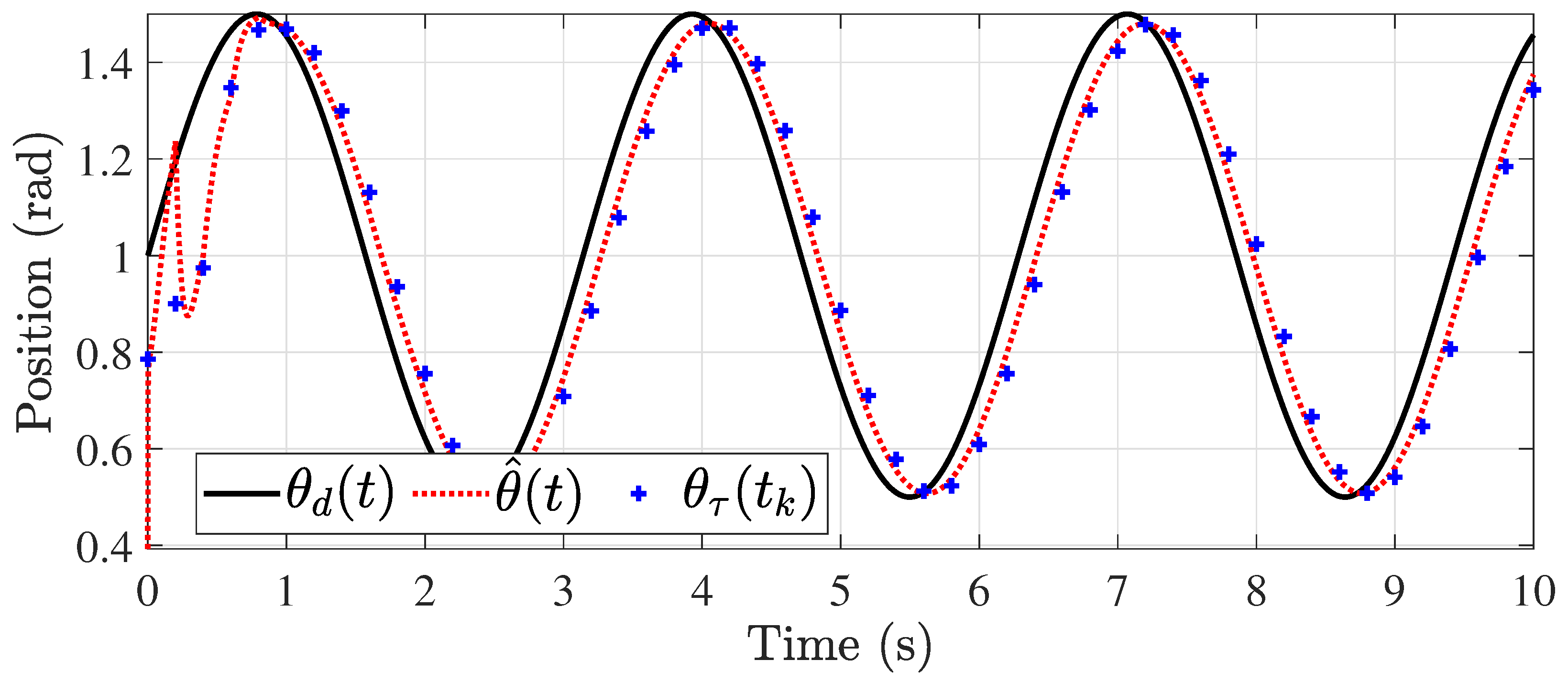
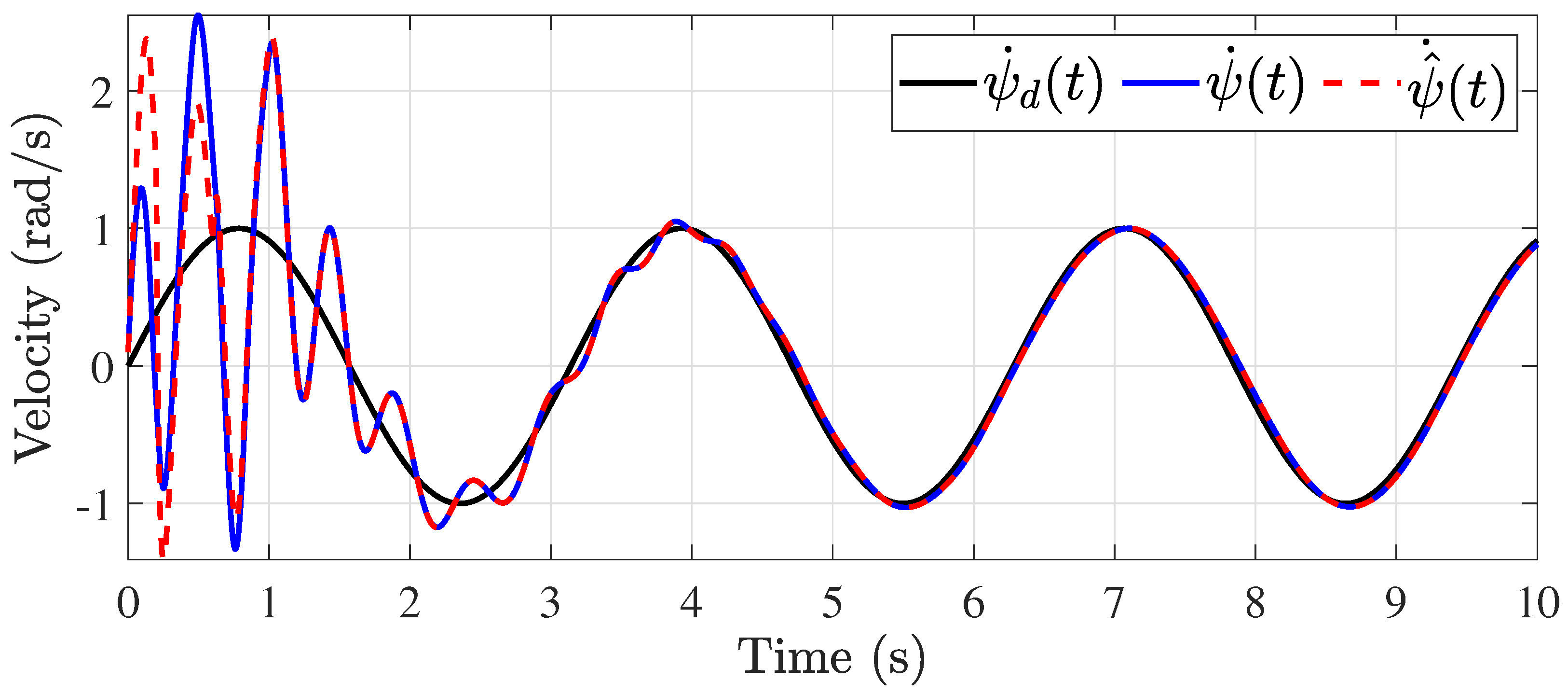
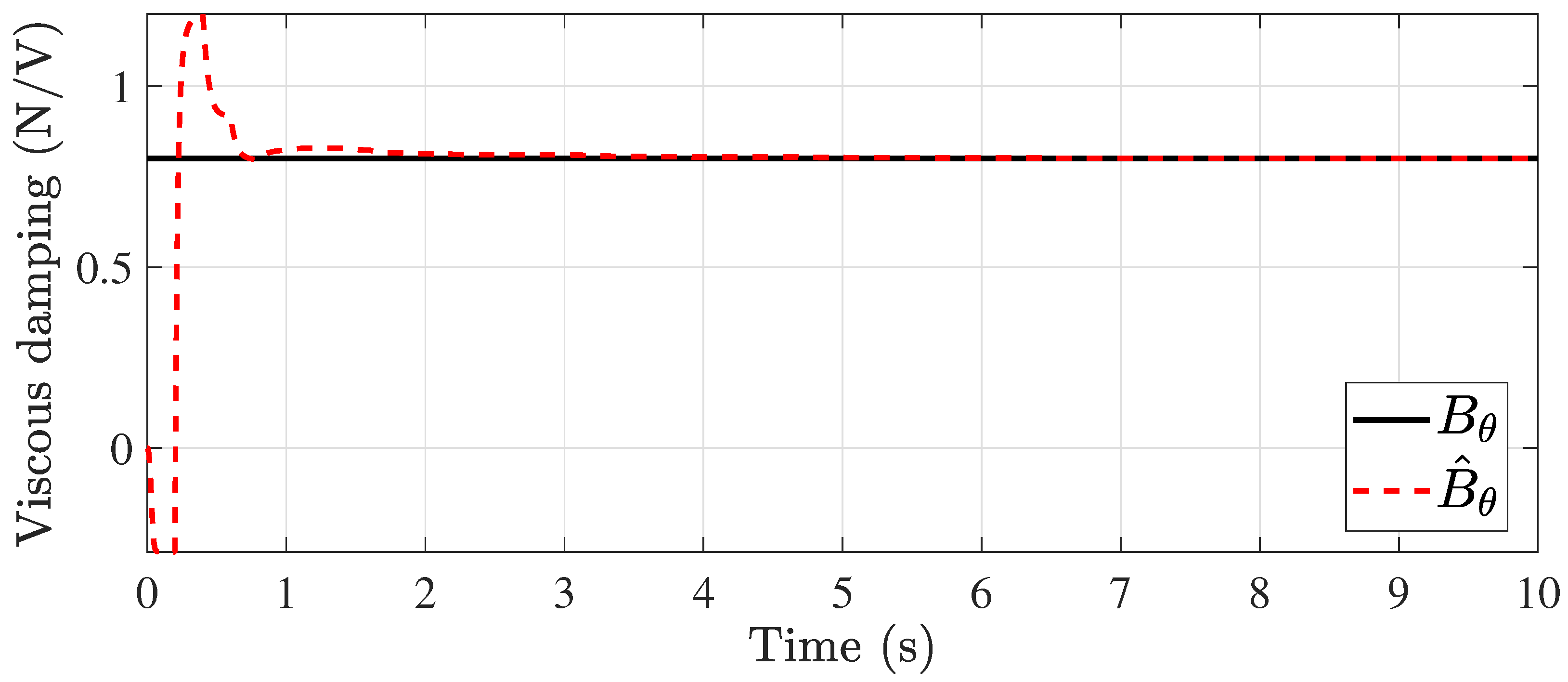
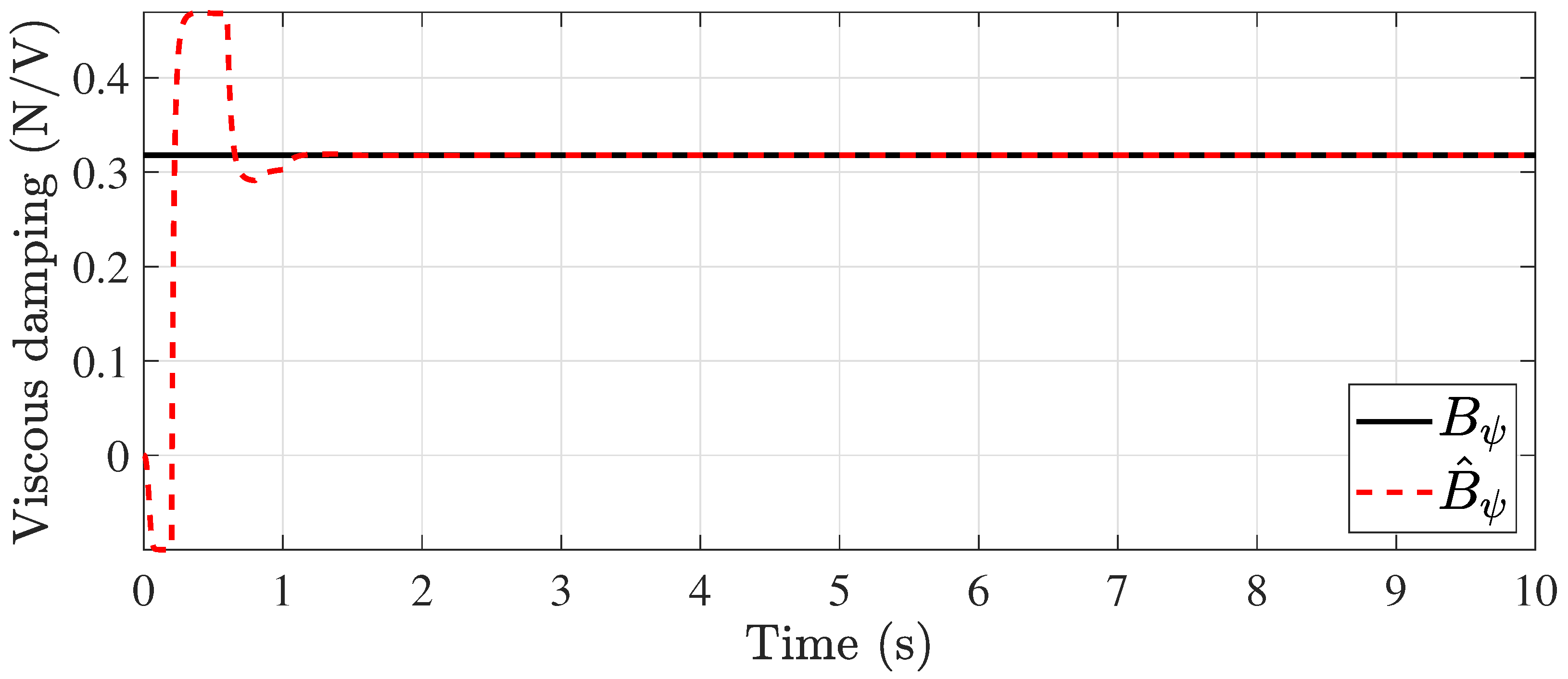
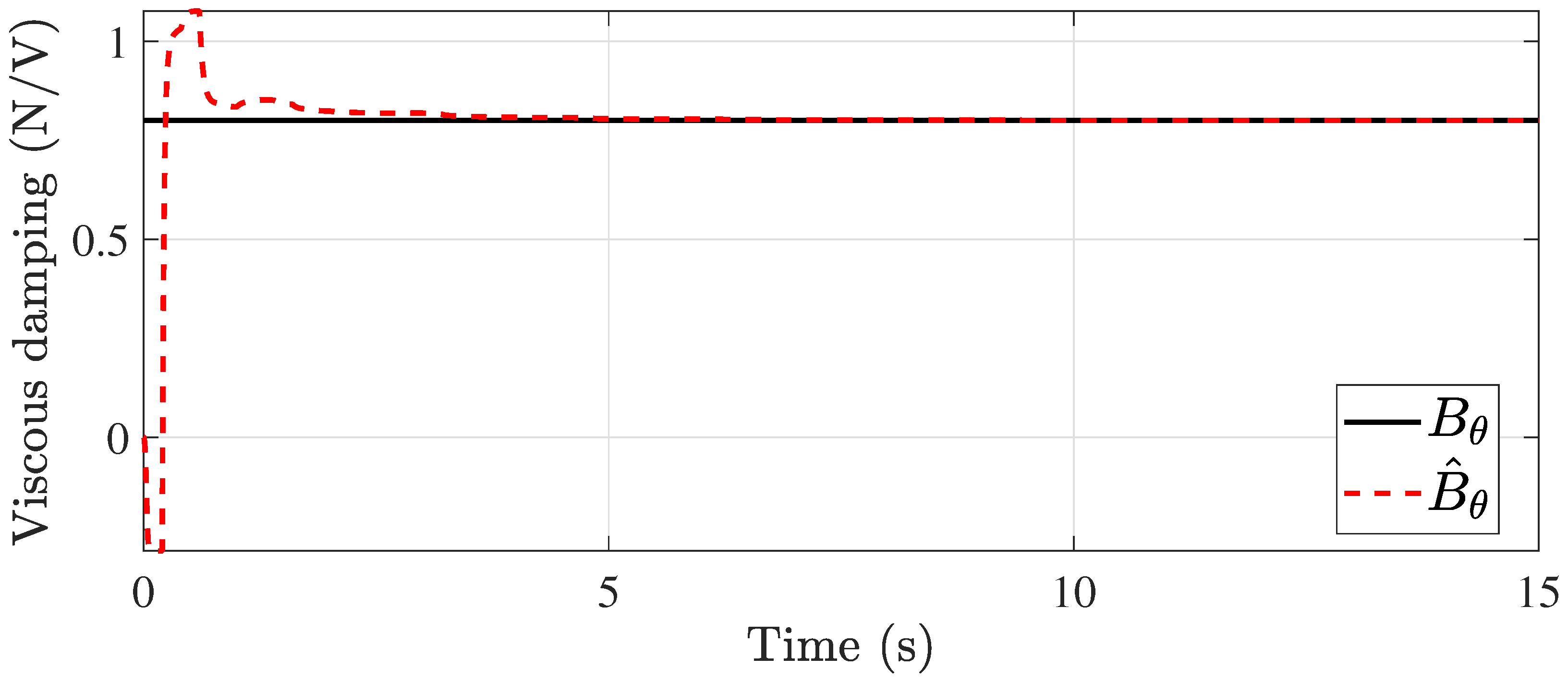
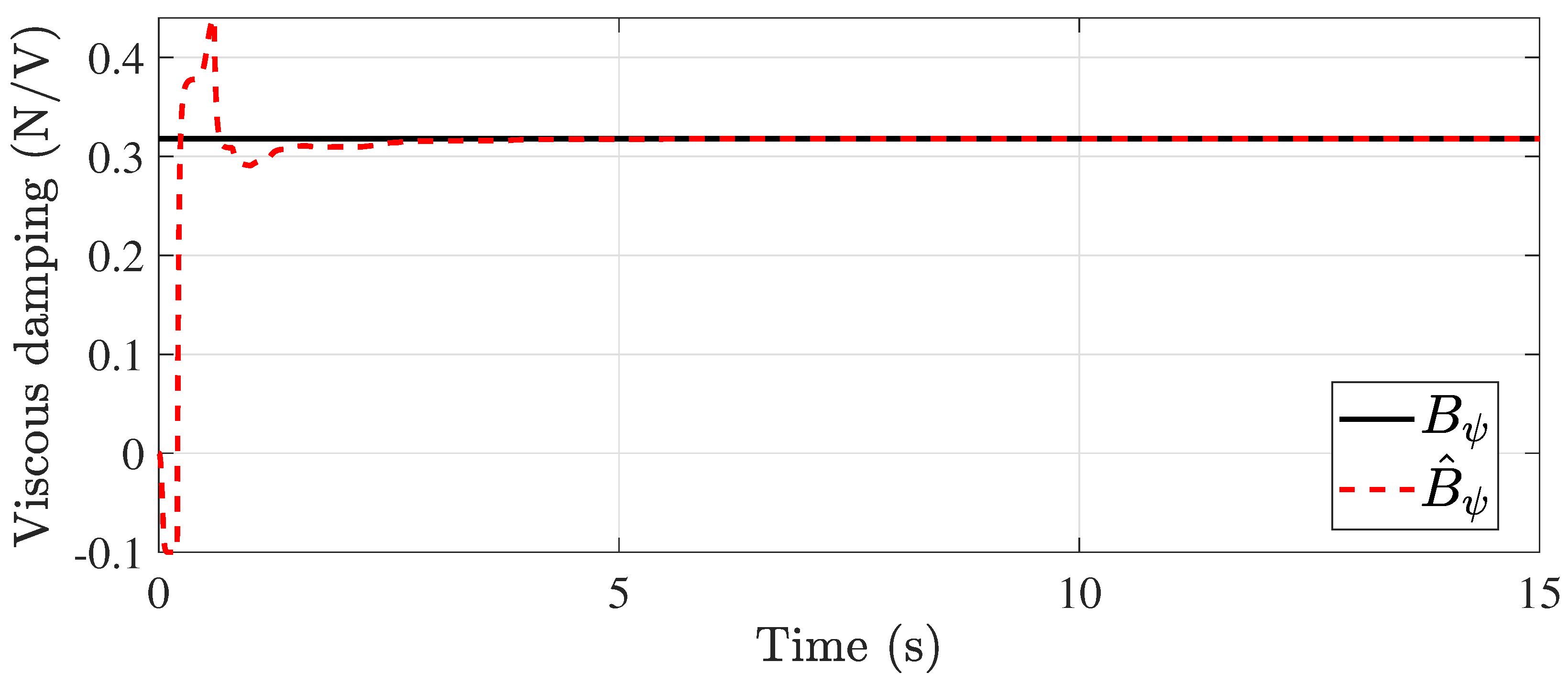
The first simulation considers the case where the control signal presents a constant delay. For this purpose, τ = 0.025 s. The simulation results are shown in Figure 2, Figure 3, Figure 4, Figure 5, Figure 6 and Figure 7. The estimate of the unknown parameters present in the input signal by the observer is shown in Figure 6 and Figure 7. The control of the pitch and yaw positions are shown in Figure 2 and Figure 3, respectively. The delayed measurements of each of them are denoted by ( · ) τ ( t k ) and are only acquired in sampled intervals as mentioned above ( Δ M ). However, the designed observer achieves the estimation continuously to control the system. The speed control is shown in Figure 4 and Figure 5. It is important to note that for PD control, the knowledge of the velocities is needed, i.e., x 2 , which, in this, case are obtained from the observer, and no other extra algorithms are needed to know these variables. The advantage of the observer structure is demonstrated in Figure 6 and Figure 7, where the estimation of the unknown values B θ and B ψ are shown, respectively. These help to achieve better control, as the θ values do not have to be increased further to reduce the error due to uncertainties.

5.2. Time-Varying Delay Case

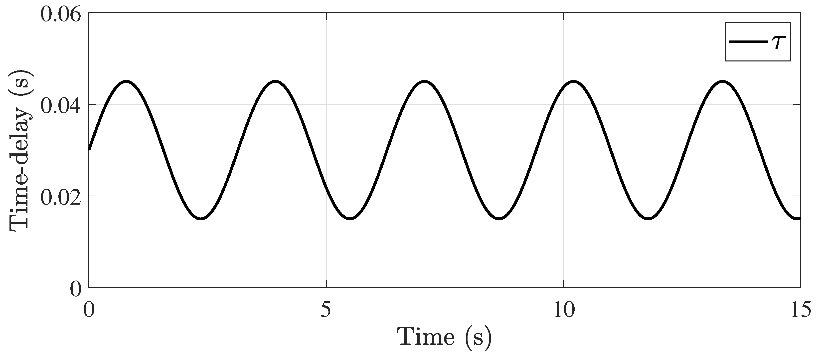
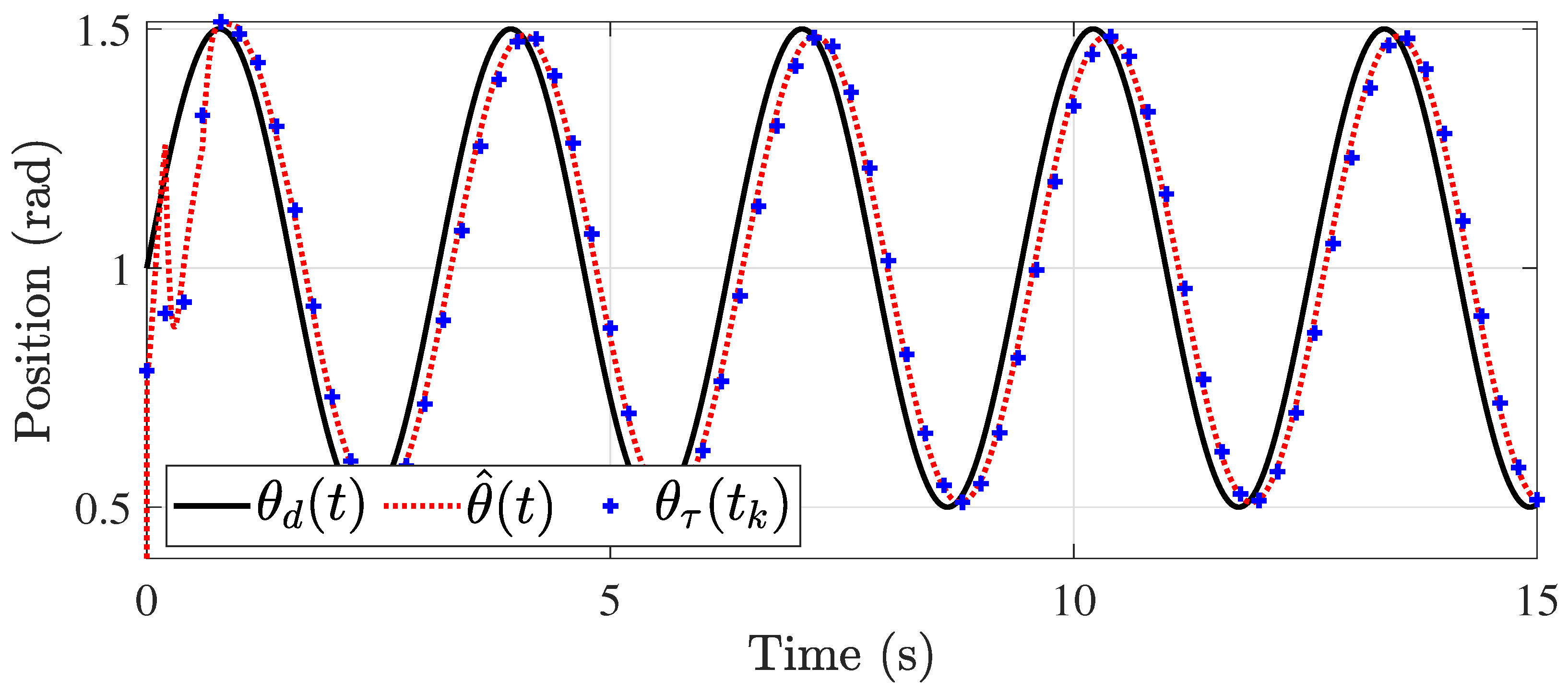
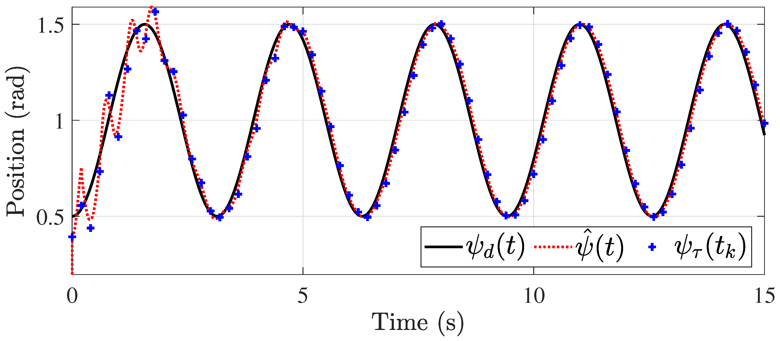
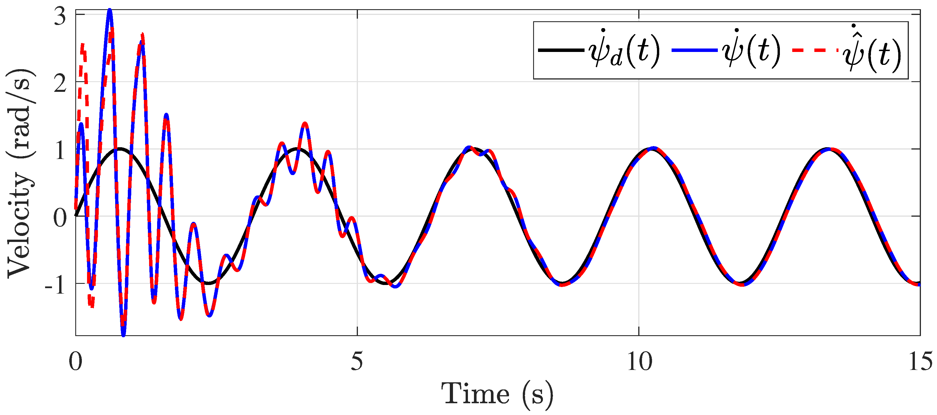
The second simulation is focused on showing the system’s effectiveness under time-varying delays in the control signal and output. For this, it is considered that the maximum delay is τ * = 0.045 s and the varying function is τ ( t ) = 0.03 + 0.015 sin ( 2 t ) as shown in Figure 8. The simulation results are shown in Figure 9, Figure 10, Figure 11, Figure 12, Figure 13 and Figure 14. The control of the pitch and yaw positions is shown in Figure 9 and Figure 10, respectively. In this case, the control is more challenging because of the higher delay values, but the control is satisfactorily achieved. This is evident in Figure 11 and Figure 12, where the velocities are shown, respectively. However, it is important to highlight that the estimation of the system uncertainties is achieved, as shown in Figure 13 and Figure 14.

6. Conclusions

The design of an observer for a class of MIMO nonlinear systems considering outputs available only at time instants and known time delays has been addressed. The originality of the work is that this observer can reconstruct the actual state vector in the presence of various problems in the output measurement, such as sampling and time-varying delays. Considering this, the proposed algorithm can be implemented in hardware with low features since the outputs are available in this way in practice. It is guaranteed that the observer error will converge to a region near the origin due to the uncertainties of the system and that the convergence rate depends on the sampling time of the original system outputs. Numerical simulations of a system consisting of a 2-DoF Helicopter are presented to test the effectiveness of the proposed algorithm. The objective of the simulation was to achieve trajectory tracking using an observer-based control and take advantage of the observer structure to estimate the uncertainties in the system. The main limitation with respect to other approaches lies in the condition of the sampling interval since, in some cases, it is not fulfilled, and the observer does not achieve convergence. Another limitation is that the system must comply with the persistent excitation condition. However, this condition can be achieved by adjusting the system inputs. Future work will address the case of even longer delays in the system output in order to address cases presented when there are long distances in the transmission networks, as well as to attenuate the effects of signals other than the output signal, such as measurement noise.

Author Contributions

Conceptualization, O.H.-G. and F.R.-R.; methodology, M.F.; software, M.-E.G.-S.; validation, C.-M.A.-Z.; formal analysis, O.H.-G.; investigation, F.R.-R.; writing—original draft preparation, M.M.; writing—review and editing, G.V.-P.; visualization, M.M.; supervision, M.-E.G.-S.; project administration, O.H-G.; funding acquisition, G.V.-P. All authors have read and agreed to the published version of the manuscript.

Funding

This research was supported by Tecnológico Nacional de México under the program Proyectos de Investigación Científica y Desarrollo Tecnológico e Innovación and the international network Red Internacional de Control y Cómputo Aplicado. Additional support was provided by Conahcyt under the program Investigadoras e Investigadores por México Project 88 and the work of Felipe Ramírez-Rasgado through a Doctoral Fellowship Assignment. Research supported in part by the “Agence Nationale de la Recherche” (ANR), Project N° ANR-19-CE10-0007-04, France.

Institutional Review Board Statement

Not applicable.

Informed Consent Statement

Not applicable.

Data Availability Statement

Data are contained within the article.

Conflicts of Interest

The authors declare no conflicts of interest.

References

  1. Abd, M.H.; Tahir, F.R.; Al-Suhail, G.A.; Pham, V.T. An adaptive observer synchronization using chaotic time-delay system for secure communication. Nonlinear Dyn. 2017, 90, 2583–2598. [Google Scholar] [CrossRef]
  2. Li, D.; Ma, W. Asymptotic properties of a HIV-1 infection model with time delay. J. Math. Anal. Appl. 2007, 335, 683–691. [Google Scholar] [CrossRef]
  3. Qi, W.; Kao, Y.; Gao, X.; Wei, Y. Controller design for time-delay system with stochastic disturbance and actuator saturation via a new criterion. Appl. Math. Comput. 2018, 320, 535–546. [Google Scholar] [CrossRef]
  4. Borri, A.; Cacace, F.; De Gaetano, A.; Germani, A.; Manes, C.; Palumbo, P.; Panunzi, S.; Pepe, P. Luenberger-like observers for nonlinear time-delay systems with application to the artificial pancreas: The attainment of good performance. IEEE Control. Syst. Mag. 2017, 37, 33–49. [Google Scholar] [CrossRef]
  5. Sanz, R.; García, P.; Fridman, E.; Albertos, P. Robust predictive extended state observer for a class of nonlinear systems with time-varying input delay. Int. J. Control. 2020, 93, 217–225. [Google Scholar] [CrossRef]
  6. Avilés, J.D.; Moreno, J.A.; Bejarano, F.J. Dissipative state observer design for nonlinear time-delay systems. J. Frankl. Inst. 2023, 360, 887–909. [Google Scholar] [CrossRef]
  7. Li, T.; Zheng, C.; Ma, Y.; Wang, Z. Interval estimation for discrete-time linear time-delay systems based on state augmentation. Eur. J. Control. 2023, 72, 100823. [Google Scholar] [CrossRef]
  8. Akbari, E.; Tabatabaei, S.M.; Yazdi, M.B.; Arefi, M.M.; Cao, J. Resilient backstepping control for a class of switched nonlinear time-delay systems under hybrid cyber-attacks. Eng. Appl. Artif. Intell. 2023, 122, 106128. [Google Scholar] [CrossRef]
  9. Di Ferdinando, M.; Di Gennaro, S.; Pepe, P. On Sontag’s formula for the sampled-data observer-based stabilization of nonlinear time-delay systems. Automatica 2023, 153, 111052. [Google Scholar] [CrossRef]
  10. Langueh, K.; Zheng, G.; Floquet, T. Impulsive fixed-time observer for linear time-delay systems. J. Frankl. Inst. 2018, 355, 3354–3366. [Google Scholar] [CrossRef]
  11. Islam, S.I.; Shi, P.; Lim, C.C. Robust functional observer for stabilising uncertain fuzzy systems with time-delay. Granul. Comput. 2020, 5, 55–69. [Google Scholar] [CrossRef]
  12. Ahmed-Ali, T.; Fridman, E.; Giri, F.; Kahelras, M.; Lamnabhi-Lagarrigue, F.; Burlion, L. Observer design for a class of parabolic systems with large delays and sampled measurements. IEEE Trans. Autom. Control. 2019, 65, 2200–2206. [Google Scholar] [CrossRef]
  13. Cacace, F.; Germani, A.; Manes, C. Predictor-based control of linear systems with large and variable measurement delays. Int. J. Control. 2014, 87, 704–714. [Google Scholar] [CrossRef]
  14. Du, S.L.; Wang, R.; Wang, S.; Yu, M. Observer-based H stabilisation for linear systems with large delay periods. IET Control. Theory Appl. 2016, 10, 417–423. [Google Scholar] [CrossRef]
  15. Liu, Q.; Zhou, B. Extended observer based feedback control of linear systems with both state and input delays. J. Frankl. Inst. 2017, 354, 8232–8255. [Google Scholar] [CrossRef]
  16. Adil, A.; Hamaz, A.; N’doye, I.; Zemouche, A.; Laleg-Kirati, T.M.; Bedouhene, F. On high-gain observer design for nonlinear systems with delayed output measurements. Automatica 2022, 141, 110281. [Google Scholar] [CrossRef]
  17. Azmi, H.; Yazdizadeh, A. Robust adaptive fault detection and diagnosis observer design for a class of nonlinear systems with uncertainty and unknown time-varying internal delay. ISA Trans. 2022, 131, 31–42. [Google Scholar] [CrossRef] [PubMed]
  18. Ghanes, M.; De Leon, J.; Barbot, J.P. Simultaneous observation and identification for nonlinear systems under unknown time-varying delays. J. Frankl. Inst. 2016, 353, 2305–2318. [Google Scholar] [CrossRef]
  19. Gamiochipi, J.; Ghanes, M.; Aggoune, W.; De Leon, J.; Barbot, J.P. Observer design for a class of nonlinear systems under a persistent excitation. IFAC-PapersOnLine 2016, 49, 517–521. [Google Scholar] [CrossRef]
  20. Yang, Y.; Lin, C.; Chen, B. Nonlinear H observer design for one-sided Lipschitz discrete-time singular systems with time-varying delay. Int. J. Robust Nonlinear Control. 2019, 29, 252–267. [Google Scholar] [CrossRef]
  21. Echi, N. Observer design and practical stability of nonlinear systems under unknown time-delay. Asian J. Control. 2021, 23, 685–696. [Google Scholar] [CrossRef]
  22. Shen, S.; Song, A.; Li, H.; Li, T. Cascade predictor for a class of mechanical systems under large uncertain measurement delays. Mech. Syst. Signal Process. 2022, 167, 108536. [Google Scholar] [CrossRef]
  23. Ramírez-Rasgado, F.; Astorga-Zaragoza, C.M.; Hernández-González, O.; Guerrero-Sánchez, M.E.; Osorio-Gordillo, G.L.; Reyes-Reyes, J. Observer Synthesis for Uncertain Nonlinear Systems with Nonuniformly Sampled and Delayed Output. IEEE Syst. J. 2022, 16, 4532–4540. [Google Scholar] [CrossRef]
  24. Nguyen, C.M.; Pathirana, P.N.; Trinh, H. Robust state estimation for non-linear systems with unknown delays. IET Control. Theory Appl. 2019, 13, 1147–1154. [Google Scholar] [CrossRef]
  25. Kalamian, N.; Khaloozadeh, H.; Ayati, M. Design of state-dependent impulsive observer for non-linear time-delay systems. IET Control. Theory Appl. 2019, 13, 3155–3163. [Google Scholar] [CrossRef]
  26. Peixoto, M.L.; Nguyen, A.T.; Guerra, T.M.; Palhares, R.M. Unknown input observers for time-varying delay Takagi-Sugeno fuzzy systems with unmeasured nonlinear consequents. Eur. J. Control. 2023, 72, 100830. [Google Scholar] [CrossRef]
  27. Dong, Y.; Hao, J.; Mei, S.; Deng, M. Observer design for one-sided Lipschitz uncertain descriptor systems with time-varying delay and nonlinear uncertainties. Circuits Syst. Signal Process. 2021, 40, 4779–4798. [Google Scholar] [CrossRef]
  28. Taghieh, A.; Shafiei, M.H. Observer-based robust model predictive control of switched nonlinear systems with time delay and parametric uncertainties. J. Vib. Control. 2021, 27, 1939–1955. [Google Scholar] [CrossRef]
  29. Yang, Y.; Lin, C.; Chen, B.; Wang, Q.G. Reduced-order observer design for a class of generalized Lipschitz nonlinear systems with time-varying delay. Appl. Math. Comput. 2018, 337, 267–280. [Google Scholar] [CrossRef]
  30. Léchappé, V.; De Leon, J.; Moulay, E.; Plestan, F.; Glumineau, A. Delay and state observation for SISO nonlinear systems with input delay. Int. J. Robust Nonlinear Control. 2018, 28, 2356–2368. [Google Scholar] [CrossRef]
  31. Farza, M.; Sboui, A.; Cherrier, E.; M’Saad, M. High-gain observer for a class of time-delay nonlinear systems. Int. J. Control. 2010, 83, 273–280. [Google Scholar] [CrossRef]
  32. Hernández-González, O.; Ramírez-Rasgado, F.; Astorga-Zaragoza, C.M.; Guerrero-Sánchez, M.E.; Valencia-Palomo, G.; Rodriguez-Mata, A.E. Observer for non-linear systems with sampled measurements: Application to the friction factor estimation of a pipeline. IET Control. Theory Appl. 2021, 15, 432–445. [Google Scholar] [CrossRef]
  33. Cacace, F.; Conte, F.; Germani, A.; Palombo, G. Delay identification for a class of nonlinear systems. Int. J. Control. 2016, 89, 2350–2359. [Google Scholar] [CrossRef]
  34. Ramírez-Rasgado, F.; Hernández-González, O.; Farza, M.; M’Saad, M.; Astorga-Zaragoza, C.; Dahhou, B. On high-gain observer redesign with respect to the nature of the available outputs. In Proceedings of the 2022 10th International Conference on Systems and Control (ICSC), Marseille, France, 23–25 November 2022; pp. 190–195. [Google Scholar] [CrossRef]
  35. Boukadida, W.; Benamor, A.; Messaoud, H.; Siarry, P. Multi-objective design of optimal higher order sliding mode control for robust tracking of 2-DoF helicopter system based on metaheuristics. Aerosp. Sci. Technol. 2019, 91, 442–455. [Google Scholar] [CrossRef]
  36. Castañeda, H.; Salas-Peña, O.S.; de León-Morales, J. Extended observer based on adaptive second order sliding mode control for a fixed wing UAV. ISA Trans. 2017, 66, 226–232. [Google Scholar] [CrossRef] [PubMed]
  37. Zhang, Y.; Li, S.; Wang, S.; Wang, X.; Duan, H. Distributed bearing-based formation maneuver control of fixed-wing UAVs by finite-time orientation estimation. Aerosp. Sci. Technol. 2023, 136, 108241. [Google Scholar] [CrossRef]
  38. Guerrero-Sánchez, M.E.; Hernández-González, O.; Valencia-Palomo, G.; López-Estrada, F.R.; Rodríguez-Mata, A.E.; Garrido, J. Filtered observer-based ida-pbc control for trajectory tracking of a quadrotor. IEEE Access 2021, 9, 114821–114835. [Google Scholar] [CrossRef]
  39. Hernández-González, O.; Guerrero-Sánchez, M.E.; Farza, M.; Ménard, T.; M’Saad, M.; Lozano, R. High gain observer for a class of nonlinear systems with coupled structure and sampled output measurements: Application to a quadrotor. Int. J. Syst. Sci. 2019, 50, 1089–1105. [Google Scholar] [CrossRef]
  40. Hashim, H.A. Exponentially stable observer-based controller for VTOL-UAVs without velocity measurements. Int. J. Control. 2023, 96, 1946–1960. [Google Scholar] [CrossRef]
  41. Aligia, D.A.; Roccia, B.A.; De Angelo, C.H.; Magallan, G.A.; Gonzalez, G.N. An orientation estimation strategy for low cost IMU using a nonlinear Luenberger observer. Measurement 2021, 173, 108664. [Google Scholar] [CrossRef]
  42. Berkane, S.; Tayebi, A.; De Marco, S. A nonlinear navigation observer using IMU and generic position information. Automatica 2021, 127, 109513. [Google Scholar] [CrossRef]
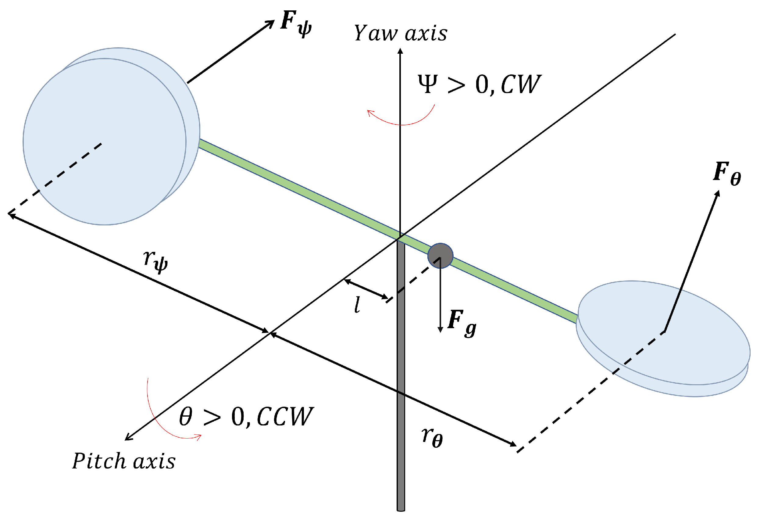
Figure 1. Free body diagram of the 2-DoF helicopter.
Aerospace 11 00206 g001
Figure 2. Tracking performance of the pitch position ( θ ) and its estimation with Δ M = 5 Hz.
Aerospace 11 00206 g002
Figure 3. Tracking performance of the yaw position ( ψ ) and its estimation with Δ M = 5 Hz.
Aerospace 11 00206 g003
Figure 4. Tracking performance of the pitch velocity ( θ ˙ ) and its estimation with Δ M = 5 Hz.
Aerospace 11 00206 g004
Figure 5. Tracking performance of the yaw velocity ( ψ ˙ ) and its estimation with Δ M = 5 Hz.
Aerospace 11 00206 g005
Figure 6. Estimation of the unknown parameter B θ with Δ M = 5 Hz.
Aerospace 11 00206 g006
Figure 7. Estimation of the unknown parameter B ψ with Δ M = 5 Hz.
Aerospace 11 00206 g007
Figure 8. Time-varying delay function.
Aerospace 11 00206 g008
Figure 9. Tracking performance of the pitch position ( θ ) and its estimation under time-varying delay.
Aerospace 11 00206 g009
Figure 10. Tracking performance of the yaw position ( ψ ) and its estimation under time-varying delay.
Aerospace 11 00206 g010
Figure 11. Tracking performance of the pitch velocity ( θ ˙ ) and its estimation under time-varying delay.
Aerospace 11 00206 g011
Figure 12. Tracking performance of the yaw velocity ( ψ ˙ ) and its estimation under time-varying delay.
Aerospace 11 00206 g012
Figure 13. Estimation of the unknown parameter B θ under time-varying delay.
Aerospace 11 00206 g013
Figure 14. Estimation of the unknown parameter B ψ under time-varying delay.
Aerospace 11 00206 g014
Table 1. Parameters of the 2-DoF helicopter.
ConstantDescriptionValueUnit
J e q , θ Total moment of inertia about pitch axis0.0384kg·m2
J e q , ψ Total moment of inertia about yaw axis0.0432kg·m2
B θ Viscous damping about pitch axis0.8000N/V
B ψ Viscous damping about yaw axis0.3180N/V
K θ θ Thrust torque of pitch motor0.2040N·m/V
K ψ ψ Thrust torque of yaw motor0.0720N·m/V
K θ ψ Thrust torque of pitch axis from yaw motor0.0068N·m/V
K ψ θ Thrust torque of yaw axis from pitch motor0.0219N·m/V
mMass of the helicopter1.3872kg
lCenter of mass length along helicopter body from a pitch axis0.1860m
gGravitational acceleration9.81m/s2
Disclaimer/Publisher’s Note: The statements, opinions and data contained in all publications are solely those of the individual author(s) and contributor(s) and not of MDPI and/or the editor(s). MDPI and/or the editor(s) disclaim responsibility for any injury to people or property resulting from any ideas, methods, instructions or products referred to in the content.