Robust Design Optimization of Viscoelastic Damped Composite Structures Integrating Model Order Reduction and Generalized Stochastic Collocation

Abstract

This study presents a novel approach that integrates model order reduction (MOR) and generalized stochastic collocation (gSC) to enhance robust design optimization (RDO) of viscoelastic damped composite structures under material and geometric uncertainties. The proposed methodology systematically reduces computational burden while maintaining the required accuracy. A projection-based MOR is chosen to alleviate the substantial computational costs associated with nonlinear eigenvalue problems. To minimize the sampling size for uncertainty propagation (UP) while effectively addressing diverse probability density distributions, a gSC method incorporating statistical moment computation techniques is developed. Pareto optimal solutions are determined by combining the proposed MOR and gSC approaches with a well-established Non-dominated Sorting Genetic Algorithm II (NSGA-II) algorithm, which accounts for robustness in handling design variables, objectives, and constraints. The results of the four examples illustrate the efficacy of the proposed MOR and gSC methods, as well as the overall RDO framework. Notably, the findings demonstrate the feasibility of this approach for practical applications, driven by a significant reduction in computational costs. This establishes a solid foundation for addressing complex optimization challenges in real-world scenarios characterized by various uncertainties.

1. Introduction

Fiber-reinforced polymer composites are increasingly employed in the aerospace industry owing to their exceptional strength-to-weight and stiffness-to-weight ratios [1]. These lightweight structures frequently endure intense vibrational environments, rendering them susceptible to structural resonance. While advanced polymeric composites possess some internal damping capacity [2], this inherent damping is often insufficient for ensuring structural safety. To effectively mitigate vibrations, the integration of viscoelastic materials into laminated structures emerges as a promising approach [3,4]. This arrangement, known as viscoelastic damped composite structures, allows for substantial shear deformation within the soft core, significantly enhancing energy dissipation efficiency. The effectiveness of such configurations is influenced by various factors, including the material properties of the viscoelastic layer, layer thickness, and the overall geometry of the composite structure. Consequently, a comprehensive understanding and optimization of these parameters are critical for improving the dynamic performance of viscoelastic damped composite structures in practical applications.

Numerical modeling and solution approaches have played a pivotal role in understanding and predicting the dynamic performance of viscoelastic damped composite structures. Recent advancements have led to the development of various efficient simplified models, such as equivalent single layer (ESL) models [5], zig-zag (ZZ) models [6], and layer-wise (LW) models [7]. Among these, the LW model has gained recognition due to its capability to automatically represent ZZ continuity throughout the thickness and accurately predict transverse stresses. A thorough review of LW theories and their numerical implementations can be found in Ref. [8]. Free vibration analysis of viscoelastic damped composite structures requires consideration of the frequency-dependent characteristics of viscoelastic materials. The introduction of these characteristics via complex material constitutive models results in a stiffness matrix that varies with the frequency parameter. Consequently, the conventional complex eigenvalue problem is transformed into a nonlinear eigenvalue problem, significantly complicating the numerical solution process. Effective solution methods for analyzing viscoelastic damped composite structures can be categorized into three main approaches: iterative solution methods [9,10,11,12,13,14,15], the contour integral method [16], and projection-based iterative solution methods [17,18,19,20,21,22,23,24,25,26,27].

• Iterative solution methods can be further categorized into fixed-point iteration, Newton iteration, and the asymptotic numerical method. The fixed-point iteration method, originating from Lin and Lim [9], is also referred to as the iterative complex eigensolution method in Ref. [10]. This method relies on an initial value assumption and iterative refinement to converge toward an accurate result. While straightforward and stable, it is also the most time-consuming approach. In contrast, the Newton iteration has a faster convergence rate but typically necessitates the computation of derivatives of the eigenvalues and eigenvectors. Detailed discussions on this method can be found in the works of Adhikari and Pascual [11] and Singh [12]. The asymptotic numerical method, also known as the high-order Newton iteration method, is a series expansion algorithm proposed by Daya and Potier-Ferry [13]. This method effectively addresses high damping and frequency-dependent damping issues through the continuous homotopy method [14]. However, it is less robust and prone to failure in scenarios with closely modal modes [15].
• The contour integral method has recently emerged as a novel solution technique for nonlinear eigenvalue problems. It generates the eigenspace using contour integrals and solves it via the Rayleigh–Ritz method, with the Sakurai–Sugiura method with the Rayleigh–Ritz projection (SSRR) algorithm introduced by Yokota and Sakurai [16] serving as a notable instance. The contour integral method offers advantages such as ease of parallelization and high computational efficiency. However, it requires subjective parameter settings, which can lead to variability in both computational stability and accuracy.
• The projection-based iterative solution method incorporates projection approximations into iterative techniques, enabling the resolution of nonlinear eigenvalue problems within a reduced subspace. Key approaches include the nonlinear Arnoldi method [17] and the nonlinear Jacobi–Davidson method [18]. Hamdaoui et al. [19] demonstrated that the computational efficiency of both the nonlinear Arnoldi and Jacobi–Davidson methods is quite similar, with both methods outperforming the asymptotic numerical method and the iterative complex eigensolution method. From the model order reduction (MOR) perspective, the Modal Strain Energy (MSE) method [20] fits within this framework, as its projection matrix construction is based on undamped or lightly damped systems of the actual structure. However, it shows reduced predictive accuracy for highly damped systems [21]. To address this limitation, Hu et al. [22] introduced a refined MSE method that accounts for damping contributions. Trindade et al. [23] proposed an iterative MSE method for active-passive vibration control problems. D’Ottavio et al. [24] utilized the iterative MSE method to the free vibration analysis of multi-core viscoelastic damped composite structures. Bilasse et al. [25] developed a series of modal projection-based reduction methods, including the real eigenmode method, improved real eigenmode method, approximate complex eigenmode method, and precise complex eigenmode method. Additionally, Boumediene et al. [26] reinforced the projection matrix with terms related to damping forces, resulting in the Enhanced MSE (E-MSE) method. A comprehensive review can be found in Ref. [27].

The flexibility of viscoelastic damped composite structures allows for effective optimization designs, which can be categorized into layout optimization for partially damped structures and parameter optimization for fully damped structures. The former primarily emphasizes damping topology optimization, which is not the focus of this article. In contrast, the latter involves critical parameter optimization, such as layer thickness and material orientation, to enhance structural performance and reduce weight. Araújo et al. [28] combined a gradient-based method with a mixed layer-wise finite element model to maximize modal loss factors, subject to specified constraints. Le Maoût et al. [29] optimized a composite sandwich plate structure using a linear search algorithm in Matlab for maximum damping loss factors. Montemurro et al. [30] integrated the genetic algorithm (GA) BIANCA method with the finite element method (FEM) for maximizing modal loss factors under stiffness and weight constraints. Hamdaoui et al. [31] focused on selecting viscoelastic materials for optimal weight and damping. Zig-zag models with FEM and Non-dominated Sorting Genetic II (NSGA-II) were used for composite beam optimization. Madeira et al. [32] conducted multi-objective designs for sandwich structures, maximizing modal loss factors while minimizing weight. Arikoglu [33] developed a multi-objective method for minimum weight and vibration response of hybrid beams using the generalized differential quadrature method. Pathan et al. [34] developed a real-coded genetic algorithm for optimal laminated composite structures. Valvano et al. [35] proposed a Decline Population Swarm Optimization method for multilayered plates, while Li and Narita [36] and Akoussan et al. [37] developed different layer-wise optimization methods for maximizing loss factors in hybrid laminated plates.

All prior studies have been conducted within a deterministic framework. However, viscoelastic damped composite structures exhibit considerable variability in materials and geometrical configurations, primarily due to the inherent randomness linked to production and processing methods. Such uncertainties can propagate through simulations during optimization loops, resulting in notable deviations from expected performance outcomes. Therefore, it is essential to develop an optimization methodology that incorporates these uncertainties in the design of viscoelastic damped composite structures.

A promising approach is robust design optimization (RDO) [38], which aims to reduce the performance sensitivity to parameter variations, thereby enhancing reliability and effectiveness in practical applications. This framework not only improves design robustness but also facilitates a deeper understanding of how uncertainties impact structural performance. Guedri et al. [39] presented a robust design methodology for mechanical structures where the uncertainties concern both the variables related to the main structure and those of viscoelastic treatments. The perturbation technique was introduced into the finite element model to perform iterative model updating. Jaboviste et al. [40] performed a robustness study using the info-gap theory to evaluate the modal damping performances for the two considered viscoelastic materials in an uncertain temperature environment.

From the only available literature, it can be noted that the substantial computational cost related to the repeated uncertainty propagation (UP) analysis during optimization iterations poses a significant challenge for RDO in viscoelastic damped composite structures. UP is a forward quantitative procedure used to predict the impact of uncertainties on responses. Currently, most UP analyses in this field primarily utilize the Monte Carlo Simulation (MCS) method, as demonstrated by Hernández et al. [41], Druesne et al. [42], and Silva et al. [43]. While MCS is favored for its straightforward implementation and high accuracy, it requires numerous evaluations of a deterministic solver across various parameter realizations, making it computationally intensive and time-consuming. To overcome this issue, we previously employed a stochastic collocation (SC) method [44] for UP analysis of modal responses [45] and frequency responses [46,47]. This approach utilizes input statistical information for sampling and polynomial basis selection, enabling the construction of a high-fidelity probabilistic surrogate model at a low computational cost. Once established, the approximation model allows for UP analysis to be conducted with negligible expense.

Despite advancements in UP analysis for viscoelastic damped composite structures, significant challenges persist, particularly when considering RDO applications. Firstly, the inherent difficulties in solving nonlinear eigenvalue problems result in prohibitive computational costs when applying the SC method in an RDO context, especially for large degrees-of-freedom (DoFs) structures. Furthermore, as the optimization process incorporates diverse material types, the emergence of unconventional random variables complicates the analysis and exposes limitations in existing SC methods. Lastly, there is a noticeable gap in research that effectively integrates UP analysis with intelligent optimization algorithms for these viscoelastic damped composite structures. To address these issues, this study introduces a novel projection-based MOR method tailored for single-sample analysis. For UP analysis, we propose a generalized stochastic collocation (gSC) method that employs statistical moment computation techniques, accommodating arbitrary random distributions. By synergistically combining model reduction techniques, advanced UP methodologies, and intelligent multi-objective optimization algorithms, this research seeks to establish a robust multi-objective optimization framework that enhances both the efficiency and reliability of viscoelastic damped composite structures.

2. Brief Review of Viscoelastic Damped Composite Structures

2.1. Viscoelastic Damping Materials

Viscoelastic damping materials are a type of polymer whose storage modulus and loss factor are significantly influenced by environmental factors such as temperature, frequency, and strain amplitude. Generally, temperature and frequency are the two most critical factors. This study primarily focuses on the effects of frequency on the performance of viscoelastic materials. It is widely recognized that changes in the frequency of applied loads do not directly alter the phase of the material but can significantly affect the motion of molecular chains, leading to observable changes in dynamic mechanical properties. In the low-frequency regime, the material behaves in a rubber-like manner, exhibiting a low storage modulus and loss factor. This behavior arises because the molecular chains can fully respond to the small frequency variations, resulting in substantial elastic deformation with negligible energy dissipation. Conversely, in the high-frequency regime, the material assumes a glassy state, marked by a significantly high storage modulus and a low loss factor. In this scenario, molecular chains cannot accommodate rapid frequency changes, resulting in limited elastic deformation and minimal energy dissipation. Within a certain frequency range, the material transitions to a glass transition state, where the storage modulus increases rapidly, and the loss factor first rises to a maximum before swiftly declining. This phenomenon occurs because the molecular chains exhibit restricted motion and cannot fully track the variations in the alternating load, leading to phase lag and increased energy dissipation.

The mechanical response of viscoelastic damping materials can be fully or partially characterized by a constitutive model using abstract mathematical language. In recent decades, several viscoelastic mathematical models have been proposed, including the Fractional Derivative model [48], the Golla–Hughes–McTavish model [49], and the Anelastic Displacement Fields model [50].

Table 1. Frequency-domain constitutive models of six viscoelastic materials [51].

Materials	Complex Modulus	Parameter	Other Properties
3M ISD-112	$G_0(1+{\displaystyle \sum _{k=1}^3\frac{{\Delta }_k\omega }{\omega -\mathrm{i}{\Omega }_k}})$	$\begin{array}{l}{G}_0=0.5 \mathrm{MPa},\\ {\Delta }_1=0.746, {\Omega }_1=468.7 \mathrm{rad}/\mathrm{s}\\ {\Delta }_2=3.265, {\Omega }_2=4742.4 \mathrm{rad}/\mathrm{s}\\ {\Delta }_3=43.284, {\Omega }_3=\mathrm{71,532.5} \mathrm{rad}/\mathrm{s}\end{array}$	$\begin{array}{l}v=0.5\\ \rho =1600{ \mathrm{kg}/\mathrm{m}}^3\end{array}$
PVB	$G_{\infty }+(G_0-G_{\infty }){(1+{(\mathrm{i}\omega \tau )}^{1-a})}^{-b}$	$\begin{array}{l}{G}_0=0.479 \mathrm{MPa},G_{\infty }=235 \mathrm{MPa},\\ \tau =0.3979 \mathrm{s},a=0.46,b=0.1946\end{array}$	$\begin{array}{l}v=0.49\\ \rho =999{ \mathrm{kg}/\mathrm{m}}^3\end{array}$
ZN-1	$G_0(1+{\displaystyle \sum _{k=1}^3{\widehat{\alpha }}_k\frac{{(\mathrm{i}\omega )}^2+2{\widehat{\zeta }}_k{\widehat{\omega }}_k\mathrm{i}\omega }{{(\mathrm{i}\omega )}^2+2{\widehat{\zeta }}_k{\widehat{\omega }}_k\mathrm{i}\omega +{\widehat{\omega }}_k^2}})$	$\begin{array}{l}{G}_0=0.5542 \mathrm{MPa}, \\ {\widehat{\alpha }}_1=3.960,{\widehat{\zeta }}_1=148.0, {\widehat{\omega }}_1=\mathrm{896,200} \mathrm{rad}/\mathrm{s}, \\ {\widehat{\alpha }}_2=65.69,{\widehat{\zeta }}_2=12.16, {\widehat{\omega }}_2=\mathrm{927,800} \mathrm{rad}/\mathrm{s},\\ {\widehat{\alpha }}_3=1.447,{\widehat{\zeta }}_3=810.4, {\widehat{\omega }}_3=\mathrm{716,300} \mathrm{rad}/\mathrm{s},\end{array}$	$\begin{array}{l}v=0.49\\ \rho =970{ \mathrm{kg}/\mathrm{m}}^3\end{array}$
DM 9740	$G_0(1+{\displaystyle \sum _{k=1}^3\frac{{\Delta }_k\omega }{\omega -\mathrm{i}{\Omega }_k}})$	$\begin{array}{l}{G}_0=1.4 \mathrm{MPa},\\ {\Delta }_1=7.262, {\Omega }_1=406.611 \mathrm{rad}/\mathrm{s}\\ {\Delta }_2=\mathrm{288,181.234}, {\Omega }_2=\mathrm{22,490,029.8} \mathrm{rad}/\mathrm{s}\\ {\Delta }_3=2.039, {\Omega }_3=46.750 \mathrm{rad}/\mathrm{s}\end{array}$	$\begin{array}{l}v=0.49\\ \rho =1101{ \mathrm{kg}/\mathrm{m}}^3\end{array}$
GE SMRD	$G_0+G_0(d-1){\displaystyle \frac{{(\mathrm{i}\omega \tau )}^{\alpha }}{1+(\mathrm{i}\omega \tau {)}^{\beta }}}$	$\begin{array}{l}{G}_0=5.0 \mathrm{MPa},d=36,\\ \alpha =0.605,\beta =0.554,\tau =2.09\times {10}^{-4} \mathrm{s}\end{array}$	$\begin{array}{l}v=0.49\\ \rho =1300{ \mathrm{kg}/\mathrm{m}}^3\end{array}$
EAR C-1002	$G_0+G_0(d-1){\displaystyle \frac{{(\mathrm{i}\omega \tau )}^{\alpha }}{1+(\mathrm{i}\omega \tau {)}^{\beta }}}$	$\begin{array}{l}{G}_0=0.8 \mathrm{MPa},d=1570,\\ \alpha =0.566,\beta =0.558,\tau =7.23\times {10}^{-10} \mathrm{s}\end{array}$	$\begin{array}{l}v=0.49\\ \rho =1300{ \mathrm{kg}/\mathrm{m}}^3\end{array}$

summarizes the constitutive models for six commonly used viscoelastic materials [51]. For clarity, the materials 3M ISD-112, PVB, ZN-1, DM 9740, GE SMRD, and EAR C-1002 are numbered as #1, #2, #3, #4, #5, and #6, respectively. Figure 1 illustrates the frequency-dependent characteristics of their storage modulus and loss factor over a range from 1 Hz to 1000 Hz. Among these materials, #6 is characterized by both low stiffness and low damping, while #2 and #5 exhibit high stiffness coupled with low damping. In contrast, #1 and #3 display low stiffness but relatively good damping properties, and #4 offers moderate stiffness with excellent damping performance. These variations in stiffness and damping characteristics are expected to significantly influence the dynamic analysis of viscoelastic damped composite structures.

2.2. Modeling and Numerical Solution

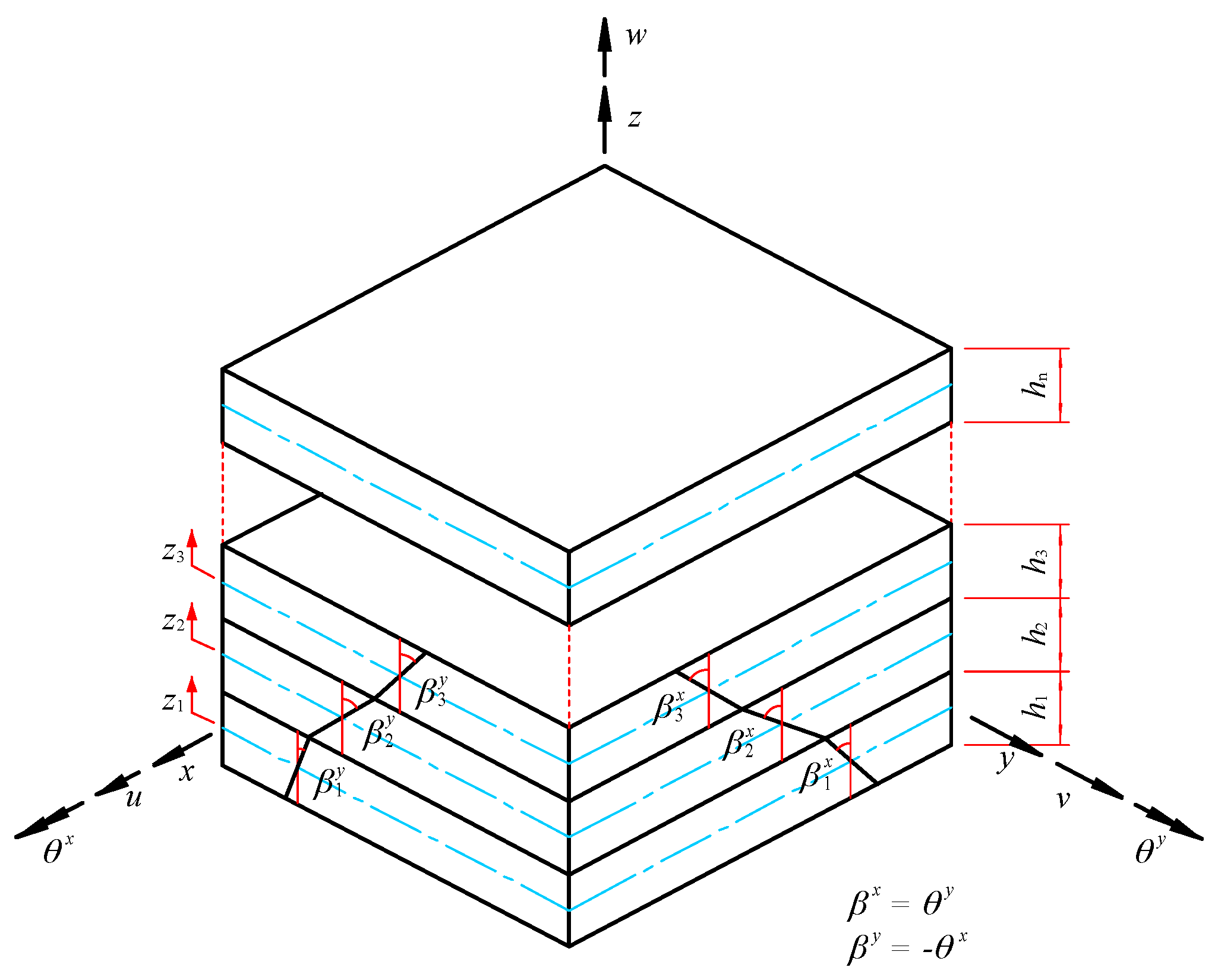
In this work, a well-validated LW finite element model, as proposed in Refs. [51,52], will be employed to model viscoelastic damped composite structures. Figure 2 presents the kinematic model of the n-layer viscoelastic damped composite structure. It is assumed that each layer follows the first-order shear deformation theory, with continuous displacements between layers. A global orthogonal coordinate system, o-xyz, is adopted, with the mid-plane of the first layer, o-xy, defined as the reference plane. The displacement of any given layer can be expressed as the sum of the displacement of the reference plane and a series of related coupled displacement terms, as shown in the equation below:

$${\mathbf{u}}_k=\left\{\begin{array}{c}{u}_k\\ v_k\\ w_k\end{array}\right\}=\left\{\begin{array}{c}{u}_0+{\displaystyle \frac{h_1}{2}}{\beta }_1^x+\sum _{j=2}^{k-1}{h}_j{\beta }_j^x+{\displaystyle \frac{h_k}{2}}{\beta }_k^x+z_k{\beta }_k^x\\ v_0+{\displaystyle \frac{h_1}{2}}{\beta }_1^y+\sum _{j=2}^{k-1}{h}_j{\beta }_j^y+{\displaystyle \frac{h_k}{2}}{\beta }_k^y+z_k{\beta }_k^y\\ w_0\end{array}\right\}$$

(1)

where $u_0$, $v_0,$ and $w_0$ represent the displacement components at the reference plane along the x, y, and z directions, respectively. The parameters ${\beta }_k^x$ and ${\beta }_k^y$ denote the angles of rotation of the normal to the mid-plane of the $k$-th layer around the y- and x-axes, respectively. $h_k$ is the thickness of the $k$-th layer, $z_k\in \left[-h_k/2,h_k/2\right]$, and $k=1,\dots ,n.$

In accordance with the conventional procedures of the finite element method, a four-node iso-parametric quadrilateral finite element is formulated, incorporating 2n + 3 DoFs for each node. Subsequently, using Hamilton’s principle, the equations of motion for the general viscoelastic damped plate are derived as follows:

$$\mathit{M}\ddot{\mathbf{u}}\left(t\right)+\mathit{K}\left(\mathrm{i}\omega \right)\mathbf{u}\left(t\right)=\mathit{f}\left(t\right)$$

(2)

where $\mathit{M}\in {\mathbb{R}}^{N\times N}$ represents the global real mass matrix with N DoFs, $\mathit{K}\left(\mathrm{i}\omega \right)\in {\mathbb{C}}^{N\times N}$ is the global complex stiffness matrix that accounts for the frequency-dependent characteristics of the viscoelastic material, $i$ denotes the imaginary unit, $\omega$ is the circular frequency, $\mathbf{u}\left(t\right)$ and $\ddot{\mathbf{u}}\left(t\right)$ are displacement and acceleration vectors, respectively, both dependent on the time $t$, $\mathit{f}\left(t\right)$ is the externally applied force. Given the free vibration of a damped viscoelastic structure, the load term on the right-hand side of the equation is equal to zero. By substituting the response $\mathbf{u}\left(t\right)=\mathbf{U}{\mathrm{e}}^{\mathrm{i}\omega t}$ into the equation, where $\mathbf{U}$ represents the amplitude vector, the eigenvalue equation is obtained as follows:

$$\left(\mathit{K}\left(\mathrm{i}\omega \right)-\lambda \mathit{M}\right)\mathit{\varphi }=\left\{\mathbf{0}\right\}$$

(3)

where $\lambda$ and $\mathit{\varphi }$ are complex eigenvalues and complex eigenvectors, respectively. The relationship between the r-th order complex eigenvalue ${\lambda }_r$ and the r-th order dynamic characteristics of the structure is shown below:

$${\lambda }_r={\omega }_r^2\left(1+\mathrm{i}{\eta }_r\right)$$

(4)

where ${\omega }_r$ is the r-th order natural frequency and ${\eta }_r$ is the r-th order modal damping ratio.

In Equation (3), $\mathit{K}\left(\mathrm{i}\omega \right)$ is a frequency-dependent function, introducing nonlinearity to the system. This makes the eigenvalue problem unsolvable through traditional methods used for linear systems with constant stiffness matrices. To overcome this, multiple iterations, commonly referred to as the Iterative Implicit Restart Arnoldi (I-IRA) method [10], are required. The entire computational process is summarized in Algorithm 1:

Algorithm 1 I-IRA method
Input:	$n$, Maximum mode order to be solved
	${\epsilon }_{\mathrm{t}}$, Convergence error tolerance
	$E_{\mathrm{V}}^{*}\left(\omega \right)$, Frequency-dependent complex modulus for viscoelastic materials
Output:	$\mathrm{First} n$ $\mathrm{natural} \mathrm{frequencies} \left\{{\omega }_1,\dots ,{\omega }_n\right\}$ $\mathrm{and} \mathrm{damping} \mathrm{ratios} \left\{{\eta }_1,\dots ,{\eta }_n\right\}$
1	$\mathrm{Set} \mathrm{the} \mathrm{initial} \mathrm{frequency} \omega =0$ Hz;
2	$\mathrm{Calculate} \mathrm{the} \mathrm{first} n$ $\mathrm{natural} \mathrm{frequencies} \left\{{\omega }_1^{\left(0\right)},\dots ,{\omega }_n^{\left(0\right)}\right\}$ (undamped system);
3	$\mathbf{For} \mathrm{each} \mathrm{mode} \mathrm{order} r=1,\dots ,n$:
4	$\mathrm{Initialize} \mathrm{the} \mathrm{iteration} \mathrm{count} i=1$ $\mathrm{and} \mathrm{the} \mathrm{modal} \mathrm{frequency} \mathrm{relative} \mathrm{error} {\epsilon }_r^{\left(1\right)}$;
5	$\mathbf{While} {\epsilon }_r^{\left(i\right)}\ge {\epsilon }_{\mathrm{t}}$:
6	$\mathrm{Substitute} {\omega }_r^{\left(i-1\right)}$ $\mathrm{into} E_{\mathrm{V}}^{*}\left(\omega \right)$ $\mathrm{to} \mathrm{obtain} \mathrm{the} \mathrm{stiffness} \mathrm{matrix} \mathit{K}\left({\omega }_r^{\left(i-1\right)}\right)$;
7	$\mathrm{Solve} \mathrm{for} \mathrm{the} \mathrm{eigenvalue} {\lambda }_r^{\left(i\right)}$ using the IRA method implemented in Matlab R2022a software;
8	$\mathrm{Compute} \mathrm{the} \mathrm{natural} \mathrm{frequency} {\omega }_r^{\left(i\right)}$ $\mathrm{and} \mathrm{relative} \mathrm{error} {\epsilon }_r^{\left(i\right)}=\left|\left({\omega }_r^{\left(i\right)}-{\omega }_r^{\left(i-1\right)}\right)/{\omega }_r^{\left(i\right)}\right|$;
9	$\mathrm{Increment} \mathrm{the} \mathrm{iteration} \mathrm{count} i=i+1$;
10	End while
11	$\mathrm{Set} {\omega }_n={\omega }_r^{\left(i-1\right)}$ $\mathrm{and} \mathrm{compute} \mathrm{the} \mathrm{damping} \mathrm{ratio} {\eta }_r$;
12	$\mathrm{Store} \mathrm{the} r\text{-}\mathrm{th} \mathrm{natural} \mathrm{frequency} {\omega }_r$ $\mathrm{and} \mathrm{the} \mathrm{damping} \mathrm{ratio} {\eta }_r$;
13	End for

3. Projection-Based Model Order Reduction Method

While the I-IRA method provides a robust solution for nonlinear eigenvalue problems, its significant computational cost, arising from multiple iterative steps, limits its feasibility in uncertainty propagation analysis and optimization design, particularly for systems with a large number of DoFs. To alleviate this computational burden, a projection-based MOR technique is proposed, which effectively reduces the dimensionality of the problem and offers a more computationally efficient approach without compromising solution accuracy.

3.1. Common Model Order Reduction Methods in Structural Dynamics

Let $n$ be the maximum mode order to be solved. For any $r$-th generalized eigenvalue problem, the projection-based MOR method posits that the required mode shape vector ${\mathit{\varphi }}_r$ can be projected into a low-dimensional subspace as follows:

$${\mathit{\varphi }}_r\approx {\mathbf{P}}_r{\mathit{\psi }}_r$$

(5)

where ${\mathbf{P}}_r$ is the $r$-th projection matrix, $\mathbf{P}\in {\mathbb{C}}^{N\times m}$ ($m\ll N$), and each column of $\mathbf{P}$ serves as an orthogonal basis for the subspace. ${\mathit{\psi }}_r$ is the $r$-th subspace coordinate vector, ${\mathit{\psi }}_r\in {\mathbb{C}}^{m\times 1}$, which determines the combination of the orthogonal basis.

To solve for ${\mathit{\varphi }}_r$, it is necessary to solve for ${\mathit{\psi }}_r$ first. Transform Equation (3) into the generalized eigenvalue equation and multiply it by ${{\mathbf{P}}_r}^T,$ yielding:

$${\overline{\mathbf{K}}}_r\left(\omega \right){\mathit{\psi }}_r={\lambda }_r{\overline{\mathbf{M}}}_r{\mathit{\psi }}_r$$

(6)

where ${\overline{\mathbf{K}}}_r\left(\omega \right)$ is the reduced frequency-dependent stiffness matrix, defined as ${\overline{\mathbf{K}}}_r\left(\omega \right)={{\mathbf{P}}_r}^T\mathbf{K}\left(\omega \right){\mathbf{P}}_r$ with ${\overline{\mathbf{K}}}_r\left(\omega \right)\in {\mathbb{C}}^{m\times m}$, ${\overline{\mathbf{M}}}_r$ is the reduced mass matrix, defined as ${\overline{\mathbf{M}}}_r={{\mathbf{P}}_r}^T\mathbf{M}{\mathbf{P}}_r$ with ${\overline{\mathbf{M}}}_r\in {\mathbb{R}}^{m\times m}$. It can be observed that through this projection transformation, the original nonlinear eigenvalue problem with $N$ DoFs is reduced to a nonlinear eigenvalue problem with $m$ DoFs. Since both the accuracy and efficiency of the solution are closely tied to the projection matrix ${\mathbf{P}}_r$, the construction of an appropriate ${\mathbf{P}}_r$ matrix is critical to this approach.

The traditional MSE method in structural dynamics constructs the projection matrix based on the undamped normal modes of the system, assuming that this projection matrix remains constant across all modal calculations:

$$\mathbf{P}={\mathbf{\Phi }}_{\mathbb{R}}=\left[{\mathit{\varphi }}_{1,\mathbb{R}},\dots ,{\mathit{\varphi }}_{nd,\mathbb{R}}\right]$$

(7)

where ${\mathbf{\Phi }}_{\mathbb{R}}$ is the matrix assembled from the normal modes of the undamped system, and $nd$ represents the maximum order of normal modes of the undamped system.

Typically, $nd$ is taken as $n$ when constructing the matrix $\mathbf{P}$. However, since the MSE method neglects the effects of damping, its direct application can lead to noticeable approximation errors when damping is pronounced or exhibits frequency-dependent characteristics. Therefore, this method is often limited to cases of low constant damping. To address this issue, Boumediene et al. [26] enhanced the projection matrix in the MSE method by incorporating terms related to the damping forces, resulting in the E-MSE method. This approach also assumes that the projection matrix for all modal calculations remains constant, where the damping-related enhancement term can be expressed as:

$${\mathbf{R}}_{\mathrm{V}}={\mathbf{K}}^{-1}\left(0\right){\tilde{\mathbf{K}}}_{\mathrm{V}}{\mathbf{\Phi }}_{\mathbb{R}}$$

(8)

Thus, the final projection matrix used in the E-MSE method can be represented as:

$$\mathbf{P}=\left[{\mathbf{\Phi }}_{\mathbb{R}},{\mathbf{R}}_{\mathrm{V}}\right]=\left[{\mathit{\varphi }}_{1,\mathbb{R}},\dots ,{\mathit{\varphi }}_{nd,\mathbb{R}},{\mathbf{K}}^{-1}\left(0\right){\tilde{\mathbf{K}}}_{\mathrm{V}}{\mathit{\varphi }}_{1,\mathbb{R}},\dots ,{\mathbf{K}}^{-1}\left(0\right){\tilde{\mathbf{K}}}_{\mathrm{V}}{\mathit{\varphi }}_{nd,\mathbb{R}}\right]$$

(9)

The E-MSE method effectively addresses the shortcomings of the original MSE approach by incorporating the influence of damping forces based on the undamped modal information. Furthermore, all enhancement terms are derived from real matrix operations, resulting in minimal computational cost. However, the E-MSE method lacks error estimation, making it challenging to apply based on actual precision requirements. Additionally, the damping force enhancement term is fixed and does not incorporate frequency-dependent aspects, which may limit its general applicability.

3.2. Proposed Projection-Based Model Order Reduction Method

Based on the considerations mentioned above, we propose a Displacement Residual Enhanced Modal Strain Energy (DRE-MSE) method built upon the MSE, E-MSE, and nonlinear Arnoldi approaches. The core idea of this method lies in reducing the original equation through the utilization of a projection basis with physical significance, encompassing the basic modal vector and the displacement residual term. As the update of the projection basis is based on the displacement residual of continuous iteration, it can gradually converge the eigensolution towards the exact solution. This dynamic adjustment effectively enhances the accuracy of modal analysis, particularly when significant damping or frequency-dependent characteristics are involved.

Algorithm 2 outlines the detailed computational process of the DRE-MSE method. Here, several important points are highlighted:

• Matrix assembly is a crucial step in the FEM process. To solve the nonlinear eigenvalue problem for the first $n$ modes, suppose that each mode requires $q$ iterations. This results in a total of $n\times q$ eigenvalue solutions. For systems with a large number of DoFs, especially when the required number of modes $n$ is substantial, the related matrix assembly in the total iterative loop can be computationally expensive. A more efficient approach is to utilize a decomposition that separates $E_{\mathrm{V}}^{*}\left(\omega \right)$ from the stiffness matrix. Since the computational cost of calculating the scalar $E_{\mathrm{V}}^{*}\left(\omega \right)$ is negligible, this significantly reduces the expense of matrix assembly during the construction of $\mathit{K}\left(\omega \right):$

  $$\mathit{K}\left(\omega \right)={\mathit{K}}_{\mathrm{E}}+E_{\mathrm{V}}^{*}\left(\omega \right){\tilde{\mathit{K}}}_{\mathrm{V}}$$

  (10)

  where ${\mathit{K}}_{\mathrm{E}}$ is the stiffness matrix associated solely with elastic materials, and ${\tilde{\mathit{K}}}_{\mathrm{V}}$ is the stiffness matrix related to viscoelastic materials, determined after introducing $E_{\mathrm{V}}^{*}\left(\omega \right)$.
• For the $r$-th reduced eigenvalue problem, as described in Equation (6), let us assume we have obtained a subspace coordinate vector ${\mathit{\psi }}_r^{\left(i\right)}$ that meets the accuracy requirements through the projection matrix ${\mathbf{P}}_r^{\left(i-1\right)}$. However, this does not imply that we can directly derive ${\mathit{\varphi }}_r^{\left(i\right)}$ using Equation (5). The influence of the iterative computation means that the order of the subspace coordinate vector obtained from the reduced eigenvalue solution may differ from that of the original modal eigenvector. To address this issue, we employ a modal tracking method to identify the matching modes. Define the correlation vector ${\mathit{v}}_{\mathit{r}}^{\left(i\right)}$ for all subspace coordinate vectors obtained at iteration step $i$ in relation to the $r$-th normal mode of the undamped system:

  $${\mathit{v}}_{\mathit{r}}^{\left(i\right)}=\left\{\left|{\mathit{\varphi }}_{r,\mathbb{R}}^T\mathbf{M}{\mathbf{P}}_r^{\left(i-1\right)}{\mathit{\psi }}_1^{\left(i\right)}\right|,\dots ,\left|{\mathit{\varphi }}_{r,\mathbb{R}}^T\mathbf{M}{\mathbf{P}}_r^{\left(i-1\right)}{\mathit{\psi }}_{2r}^{\left(i\right)}\right|\right\}$$

  (11)

  This correlation vector enables us to effectively compare and match the reduced eigenvalue solutions with the original modal shapes, ensuring that we correctly associate the computed modes with their corresponding physical counterparts.
• It is essential to select an appropriate initial projection matrix ${\mathbf{P}}^{\left(0\right)}$. Note that the column counts of the ${\mathit{v}}_{\mathit{r}}^{\left(i\right)}$ in Equation (11) expand to 2$r$, primarily to mitigate situations where the order of certain modes may change significantly. Given that the maximum value of $r$ is $n$, the initial projection matrix should have at least 2$n$ columns. As the selection of the initial projection matrix is based on the E-MSE method, which typically requires twice the maximum modal order, ${\mathbf{P}}^{\left(0\right)}$ here needs $⌊1.5n⌋$ modal modes, represented as follows:

  $${\mathbf{P}}^{\left(0\right)}=\left[{\mathit{\varphi }}_{1,\mathbb{R}},\dots ,{\mathit{\varphi }}_{⌊1.5n⌋,\mathbb{R}},{\mathit{K}}^{-1}\left(0\right){\tilde{\mathit{K}}}_{\mathrm{V}}{\mathit{\varphi }}_{1,\mathbb{R}},\dots ,{\mathit{K}}^{-1}\left(0\right){\tilde{\mathit{K}}}_{\mathrm{V}}{\mathit{\varphi }}_{⌊1.5n⌋,\mathbb{R}}\right]$$

  (12)

  where $⌊·⌋$ denotes the floor function, indicating the largest integer less than or equal to the argument.
• The key aspect of the DRE-MSE method lies in enhancing the projection matrix through the inclusion of the displacement residual term, which is derived from the force residual term. The force residual term can be computed as:

  $${\mathbf{R}\mathbf{F}}_r^{\left(i\right)}=\mathit{K}\left({\omega }_r^{\left(i\right)}\right){\mathit{\varphi }}_r^{\left(i\right)}-{\lambda }_r^{\left(i\right)}\mathbf{M}{\mathit{\varphi }}_r^{\left(i\right)}$$

  (13)

  Next, the displacement residual term can be obtained by multiplying the inverse of the stiffness matrix by the force residual term:

  $${\mathbf{R}\mathbf{U}}_r^{\left(i\right)}={\mathit{K}}^{-1}\left({\omega }_r^{\left(i\right)}\right)·\left({\mathbf{R}\mathbf{F}}_r^{\left(i\right)}\right)$$

  (14)

  However, since $\mathit{K}\left({\omega }_r^{\left(i\right)}\right)$ is a complex matrix, inverting it repeatedly during the iterative process can be computationally expensive. Therefore, this study adopts a method that only inverts the real part of the stiffness matrix:

  $${\mathbf{R}\mathbf{U}}_r^{\left(i\right)}={\left[\mathrm{R}\mathrm{e}\left(\mathit{K}\left({\omega }_r^{\left(i\right)}\right)\right)\right]}^{-1}·\left({\mathbf{R}\mathbf{F}}_r^{\left(i\right)}\right)$$

  (15)

  where $\mathrm{R}\mathrm{e}\left(·\right)$ denotes the operator that extracts the real part of a complex number.

Algorithm 2 DRE-MSE method
Input:	$n$, Maximum mode order to be solved
	${\epsilon }_{\mathrm{t}}$, Convergence error tolerance
	$E_{\mathrm{V}}^{*}\left(\omega \right)$, Frequency-dependent complex modulus for viscoelastic materials
Output:	$\mathrm{First} n$ $\mathrm{natural} \mathrm{frequencies} \left\{{\omega }_1,\dots ,{\omega }_n\right\}$ $\mathrm{and} \mathrm{damping} \mathrm{ratios} \left\{{\eta }_1,\dots ,{\eta }_n\right\}$
1	$\mathrm{Set} \mathrm{the} \mathrm{initial} \mathrm{frequency} \omega =0$ Hz;
2	$\mathrm{Calculate} \mathrm{the} \mathrm{first} ⌊1.5n⌋$ $\mathrm{eigensolutions} \mathrm{to} \mathrm{obtain} \left\{{\omega }_1^{\left(0\right)},\dots ,{\omega }_n^{\left(0\right)}\right\}$ $\mathrm{and} \left\{{\mathit{\varphi }}_{1,\mathbb{R}},\dots ,{\mathit{\varphi }}_{⌊1.5n⌋,\mathbb{R}}\right\}$;
3	$\mathrm{Compute} \mathrm{the} \mathrm{stiffness} \mathrm{matrix} {\mathit{K}}_{\mathrm{E}}$ $\mathrm{and} \mathrm{the} \mathrm{real} \mathrm{stiffness} \mathrm{matrix} {\tilde{\mathit{K}}}_{\mathrm{V}}$;
4	$\mathrm{Initialize} \mathrm{the} \mathrm{projection} \mathrm{basis} \mathrm{matrix} {\mathbf{P}}^{\left(0\right)}=\left[{\mathit{\varphi }}_{1,\mathbb{R}},\dots ,{\mathit{\varphi }}_{⌊1.5n⌋,\mathbb{R}},{\mathit{K}}^{-1}\left(0\right){\tilde{\mathit{K}}}_{\mathrm{V}}{\mathit{\varphi }}_{1,\mathbb{R}},\dots ,{\mathit{K}}^{-1}\left(0\right){\tilde{\mathit{K}}}_{\mathrm{V}}{\mathit{\varphi }}_{⌊1.5n⌋,\mathbb{R}}\right]$ and perform Gram–Schmidt orthogonalization;
5	$\mathbf{For} \mathrm{each} \mathrm{mode} \mathrm{order} r=1,\dots ,n$:
6	$\mathrm{Initialize} \mathrm{the} \mathrm{iteration} \mathrm{count} i=1$ $\mathrm{and} \mathrm{the} \mathrm{modal} \mathrm{frequency} \mathrm{relative} \mathrm{error} {\epsilon }_r^{\left(1\right)}$;
7	$\mathrm{Set} {\mathbf{P}}_r^{\left(0\right)}={\mathbf{P}}^{\left(0\right)}$;
8	$\mathbf{While} {\epsilon }_r^{\left(i\right)}\ge {\epsilon }_{\mathrm{t}}$:
9	$\mathrm{Substitute} {\omega }_r^{\left(i-1\right)}$ $\mathrm{into} E_{\mathrm{V}}^{*}\left(\omega \right)$ $\mathrm{and} \mathrm{obtain} \mathit{K}\left({\omega }_r^{\left(i-1\right)}\right)$ through matrix assemblies;
10	$\mathrm{Left}\text{-}\mathrm{multiply} \mathrm{Equation} (3) \mathrm{by} {{\mathbf{P}}_r^{\left(i-1\right)}}^T$ to obtain Equation (6);
11	$\mathrm{Calculate} \mathrm{the} \mathrm{first} 2r$ $\mathrm{eigenvalues} \left\{{\lambda }_1^{\left(i\right)},\dots ,{\lambda }_{2r}^{\left(i\right)}\right\}$ $\mathrm{and} \mathrm{reduced} \mathrm{vectors} \left\{{\mathit{\psi }}_1^{\left(i\right)},\dots ,{\mathit{\psi }}_{2r}^{\left(i\right)}\right\}$;
12	$\mathrm{Conduct} \mathrm{mode} \mathrm{tracking} \mathrm{by} \mathrm{calculating} \mathrm{the} \mathrm{correlation} \mathrm{vector} {\mathit{v}}_{\mathit{r}}^{\left(i\right)}=\left\{\left|{\mathit{\varphi }}_{r,\mathbb{R}}^T\mathbf{M}{\mathbf{P}}_r^{\left(i-1\right)}{\mathit{\psi }}_1^{\left(i\right)}\right|,\dots ,\left|{\mathit{\varphi }}_{r,\mathbb{R}}^T\mathbf{M}{\mathbf{P}}_r^{\left(i-1\right)}{\mathit{\psi }}_{2r}^{\left(i\right)}\right|\right\}$;
13	$\mathrm{Find} \mathrm{the} \mathrm{index} p$ $\mathrm{of} \mathrm{the} \mathrm{maximum} \mathrm{value} \mathrm{in} {\mathit{v}}_{\mathit{r}}^{\left(i\right)}$ $\mathrm{and} \mathrm{update} {\lambda }_r^{\left(i\right)}={\lambda }_p^{\left(i\right)}$ $, {\mathit{\varphi }}_r^{\left(i\right)}={\mathbf{P}}_r^{\left(i-1\right)}{\mathit{\psi }}_p^{\left(i\right)}$;
14	$\mathrm{Solve} \mathrm{for} \mathrm{the} \mathrm{eigenvalue} {\lambda }_r^{\left(i\right)}$ using the IRA method implemented in Matlab software;
15	$\mathrm{Compute} \mathrm{the} \mathrm{natural} \mathrm{frequency} {\omega }_r^{\left(i\right)}$$, \mathrm{and} \mathrm{relative} \mathrm{error} {\epsilon }_r^{\left(i\right)}=\left|\left({\omega }_r^{\left(i\right)}-{\omega }_r^{\left(i-1\right)}\right)/{\omega }_r^{\left(i\right)}\right|$;
16	$\mathrm{Compute} \mathrm{the} \mathrm{force} \mathrm{residual} {\mathbf{R}\mathbf{F}}_r^{\left(i\right)}=\mathit{K}\left({\omega }_r^{\left(i\right)}\right){\mathit{\varphi }}_r^{\left(i\right)}-{\lambda }_r^{\left(i\right)}\mathbf{M}{\mathit{\varphi }}_r^{\left(i\right)}$;
17	$\mathrm{Compute} \mathrm{the} \mathrm{approximate} \mathrm{displacement} \mathrm{residual} \mathrm{vector} {\mathbf{R}\mathbf{U}}_r^{\left(i\right)}={\left[\mathrm{R}\mathrm{e}\left(\mathit{K}\left({\omega }_r^{\left(i\right)}\right)\right)\right]}^{-1}·\left({\mathbf{R}\mathbf{F}}_r^{\left(i\right)}\right)$;
18	$\mathrm{Update} \mathrm{the} \mathrm{projection} \mathrm{basis} {\mathbf{P}}_r^{\left(i\right)}=\left[{\mathbf{P}}_r^{\left(i-1\right)},{\mathbf{R}\mathbf{U}}_r^{\left(i\right)}\right]$ and perform Gram–Schmidt orthogonalization;
19	$\mathrm{Increment} \mathrm{the} \mathrm{iteration} \mathrm{count} i=i+1$;
20	End while
21	$\mathrm{Set} {\omega }_r={\omega }_r^{\left(i-1\right)}$ $\mathrm{and} {\eta }_r={\eta }_r^{\left(i-1\right)}$;
22	$\mathrm{Store} \mathrm{the} r\text{-}\mathrm{th} \mathrm{natural} \mathrm{frequency} {\omega }_r$ $\mathrm{and} \mathrm{the} \mathrm{damping} \mathrm{ratio} {\eta }_r$;
23	End for

4. Uncertainty Propagation and Robust Design Optimization

4.1. Generalized Stochastic Collocation Method for Uncertainty Propagation

The SC method is gradually emerging as a mainstream technique in uncertainty propagation analysis. Nonetheless, the standard SC method is limited to scenarios where input random variables conform to five common probability density distributions (PDFs). This limitation restricts its applicability to viscoelastic damped composite structures that exhibit a range of uncommon probability density distributions. To address these challenges, this section presents a gSC method suitable for arbitrary random distributions. The core of the gSC method lies in its ability to solve Gauss integral nodes and weight coefficients corresponding to any random distribution by employing statistical moment computation techniques based on Fejér integration [53] and the Golub–Welsch algorithm [54], as well as by employing sparse grid techniques to generate multidimensional interpolation points.

4.1.1. The Stochastic Collocation Method

Consider a complete probability space $\left(\mathrm{\Omega },\mathcal{F},\mathcal{P}\right)$, where $\mathrm{\Omega }$ is the sample space, $\mathcal{F}\subset 2^{\mathrm{\Omega }}$ is a $\mathrm{\sigma }$-algebra, and $\mathcal{P}:\mathcal{F}\to \left[0,1\right]$ is a probability measure. Let $f:{\mathbb{R}}^d\to {\mathbb{R}}^1$ represent the system model. The input uncertainty of the system is defined by a random vector $\mathit{X}=\left\{X^{\left(1\right)},\dots ,X^{\left(d\right)}\right\}$ comprising $d\in {\mathbb{N}}^{+}$ independent random variables, where ${\mathrm{\Gamma }}^{\left(k\right)}=X^{\left(k\right)}\left(\mathrm{\Omega }\right)$ and ${\pi }_{X^{\left(k\right)}}\left(x^{\left(k\right)}\right)$ denotes the random domain and PDF of $X^{\left(k\right)}$, respectively. The random domain $D={\prod }_{k=1}^d{D}^{\left(k\right)}$ and the joint PDF ${\pi }_{\mathit{X}}\left(\mathit{x}\right)=\prod _{k=1}^d{\pi }_{X^{\left(k\right)}}\left(x^{\left(k\right)}\right)$ characterize the random vector $\mathit{X}$. Let ${\mathbf{\Theta }}_d=\left\{{\mathit{x}}_j\right\},j=1,\dots ,M,$ represent a set of $M$ sample points in the space $\mathrm{\Omega }$, with $\mathit{x}=\left(x^{\left(1\right)},\dots ,x^{\left(d\right)}\right)\in D\subset {\mathbb{R}}^d$ as the input sample coordinates for $k=1,\dots ,d$. The system response uncertainty is modeled as a random variable $Y$, and $y\subset {\mathbb{R}}^1$ denotes the response sample coordinates. The SC method begins with the Lagrange interpolation approximation of the system response:

$$f\left(\mathit{x}\right)\approx {\sum }_{s=1}^M{a}_s{\mathit{L}}_s\left(\mathit{x}\right)$$

(16)

where $a_s$ and ${\mathit{L}}_s\left(\mathit{x}\right)$ represent the interpolation coefficient and Lagrange polynomial basis function at the $s$-th interpolation point ${\mathit{x}}_s$, respectively. Define $\mathbb{E}$ as the expectation operator. The $p\in \mathbb{N}$ statistical moment of the system response can be expressed as:

$$\mathbb{E}\left(f^p\left(\mathit{X}\right)\right)\approx {\int }_D{\sum }_{s=1}^M{f}^p\left({\mathit{x}}_s\right){\mathit{L}}_s\left(\mathit{x}\right){\pi }_{\mathit{X}}\left(\mathit{x}\right)d\mathit{x}={\sum }_{s=1}^M{f}^p\left({\mathit{x}}_s\right){\int }_D{\mathit{L}}_s\left(\mathit{x}\right){\pi }_{\mathit{X}}\left(\mathit{x}\right)d\mathit{x}$$

(17)

The integral calculation in the above expression requires the use of weighted numerical integration. If the selected interpolation points coincide with the integration nodes, we can leverage the properties of the Lagrange basis functions to obtain:

$$\mathbb{E}\left(f\left(\mathit{X}\right)\right)\approx {\sum }_{s=1}^{M}f\left({\mathit{x}}_s\right)w_s$$

(18)

where $w_s$ denotes the weight associated with the $s$-th integration node. It is evident that this method requires evaluating the system response $M$ times to compute the first $p$ statistical moments. Thus, selecting interpolation points such that $M$ remains sufficiently small while meeting the accuracy requirements is critical to the effectiveness of this method. As mentioned, it is essential for the interpolation points to coincide with the integration nodes. In the case of one-dimensional problems, appropriate Gauss-type quadrature can be employed for commonly encountered types of random variables to directly obtain the corresponding moments. The challenge lies in devising an optimal strategy to extend these methods into multidimensional spaces while minimizing the number of nodes utilized.

When $d>1$, let $i_k$ denote the interpolation accuracy level in the $k$-th dimension, where $k=1,\dots ,d$. The coordinate set for each dimension can be defined as ${\mathrm{\Theta }}^{i_k}=\left\{x_1^{i_k},\dots ,x_{m_{i_k}}^{i_k}\right\}$, where the number of coordinates is $m_{i_k}=g\left(i_k\right)$. The full tensor product operation is the most straightforward method for constructing multidimensional interpolation points. However, it incurs significant computational costs due to the curse of dimensionality. To address this issue, sparse grid techniques have been introduced. The Smolyak algorithm [55] is a tensor-product linear combination technique for constructing coefficient grids. In interpolation applications, it achieves high approximation accuracy with significantly fewer interpolation points. Define $\mathbf{i}=\left(i_1,\dots ,i_d\right)\in {\mathbb{N}}^d$ as a multi-index vector, where each component $i_k$ represents the interpolation accuracy level in the $k$-th dimension. Let $\left|\mathbf{i}\right|=i_1+\cdots +i_d$ and define $q\in \mathbb{N}$ as the overall accuracy level. The SC method based on the isotropic Smolyak algorithm for approximating the system response through multidimensional Lagrange interpolation can be expressed as:

$${\mathrm{A}}_{q,d}\left(f\right)\left(\mathit{x}\right)={\sum }_{q+1\le \left|\mathbf{i}\right|\le q+d}{\left(-1\right)}^{q+d-\left|\mathbf{i}\right|}\left(\begin{array}{c}d-1\\ q+d-\left|\mathbf{i}\right|\end{array}\right)·\left(u^{i_1}\otimes \cdots \otimes u^{i_d}\right)\left(f\right)\left(\mathit{x}\right)$$

(19)

where ${\mathrm{A}}_{q,d}\left(f\right)\left(\mathit{x}\right)$ is the sparse grid approximation of the $d$-dimensional function $f\left(\mathit{x}\right)$ at the $q$ interpolation accuracy level. Subsequently, the first $p$ statistical moments of the approximate response can be calculated as follows:

$$\mathbb{E}\left(f^p\left(\mathit{X}\right)\right)\approx {\sum }_{q+1\le \left|\mathbf{i}\right|\le q+d}\left[{\left(-1\right)}^{q+d-\left|\mathbf{i}\right|}\left(\begin{array}{c}d-1\\ q+d-\left|\mathbf{i}\right|\end{array}\right){\sum }_{s_1=1}^{m_{i_1}}\cdots {\sum }_{s_d=1}^{m_{i_d}}{f}^p\left(x_{s_1}^{i_1},\cdots ,x_{s_d}^{i_d}\right)·\left(w_{s_1}^{i_1}\times \cdots \times w_{s_d}^{i_d}\right)\right]$$

(20)

where $s_{s_k}^{i_k}$ represents the $s_k$-th coordinate at the $i_k$ interpolation accuracy level in the $k$-th dimension, and $w_{s_k}^{i_k}$ denotes the $s_k$-th weight coefficient at the $i_k$ interpolation accuracy level in the $k$-th dimension.

In this case, the set of interpolation points for the sparse grid can be represented as:

$${\mathbf{\Theta }}_d=\mathcal{H}\left(q+d,d\right)={\bigcup }_{q+1\le \left|\mathbf{i}\right|\le q+d}{\mathrm{\Theta }}^{i_1}\times \cdots \times {\mathrm{\Theta }}^{i_d}$$

(21)

where $\mathcal{H}\left(q+d,d\right)$ denotes the set of sparse grid interpolation points in $d$ dimensions at the $q$ accuracy level.

4.1.2. The Fejér Integration for Arbitrary Random Variables

The Fejér integration is used here to calculate the higher moments of an arbitrary distribution. Considering an arbitrary random variable $X$ with a PDF ${\pi }_X\left(x\right)$ defined over the interval $\left[a,b\right]$, where $-\mathrm{\infty }\le a\le b\le \mathrm{\infty }$, the $t$-th moment ${\mu }_t$ of the input uncertainty can be expressed as:

$${\mu }_t=\mathbb{E}\left(X^t\right)={\int }_a^b{x}^t{\pi }_X\left(x\right)dx$$

(22)

It is evident that solving this one-dimensional integral analytically is quite challenging, necessitating the use of numerical integration techniques. However, when the PDF of the random variable is complex, employing Gaussian or Newton–Cotes integration for calculating higher-order statistical moments may not be reliable or practical. In such cases, using Fejér-type integrals [53,56] based on Chebyshev nodes over the interval $\left[-\mathrm{1,1}\right]$ is a preferable approach. For $n$ integration points in Fejér integrals, the $s$-th integration coordinate $z_s$ and the corresponding weight $w_s$ can be expressed as follows:

$$\left\{\begin{array}{c}{z}_s=cos\left({\displaystyle \frac{\left(2s-1\right)\mathrm{\pi }}{2n}}\right) \\ w_s={\displaystyle \frac{2}{n}}\left(1-2\sum _{k=1}^{⌊n/2⌋}{\displaystyle \frac{cos\left(2k\frac{2s-1}{2n}\right)}{4k^2-1}}\right)\end{array}\right.$$

(23)

By substituting the integration nodes and weights into Equation (22) for numerical integration, we obtain:

$${\mu }_t=\mathbb{E}\left(X^t\right)={\int }_{-1}^1{\left(\psi \left(z\right)\right)}^t\pi \left(\psi \left(z\right)\right){\psi }^{\prime }\left(z\right)dz={\sum }_{s=1}^n{\left(\psi \left(z_s\right)\right)}^t\pi \left(\psi \left(z_s\right)\right){\psi }^{\prime }\left(z_s\right)w_s$$

(24)

where $\psi \left(z\right)$ is the variable transformation function that maps $x:\left[a,b\right]$ to $z:\left[-\mathrm{1,1}\right]$, and ${\psi }^{\prime }\left(z\right)$ is the derivative of $\psi \left(z\right)$. Depending on the values of the lower limit $a$ and the upper limit $b$, $\psi \left(z\right)$ can be expressed as follows:

$$\psi \left(z\right)=\left\{\begin{array}{c}{\displaystyle \frac{b-a}{2}}z+{\displaystyle \frac{b+a}{2}},\mathrm{if}-\infty <\mathrm{a}<\mathrm{b}<\infty \\ b-{\displaystyle \frac{1-z}{1+z}},\mathrm{if}-\infty =\mathrm{a}<\mathrm{b}<\infty \\ a+{\displaystyle \frac{1+z}{1-z}},\mathrm{if}-\infty <\mathrm{a}<\mathrm{b}=\infty \\ {\displaystyle \frac{z}{1-z^2}},\mathrm{if}-\infty =\mathrm{a}<\mathrm{b}=\infty \end{array}\right.$$

(25)

4.1.3. The Golub–Welsch Algorithm

The Golub–Welsch algorithm [54] derives the corresponding Gauss integration rules from the moment information of random variables calculated by Fejér integration. This algorithm consists of two main parts: first, it derives the three-term recurrence relation for orthogonal polynomials based on the Mysovskih theory [57] from the moment information; second, it calculates the Gauss integration coordinates and weight coefficients using the recurrence coefficients. Let $\left\{{\varphi }_k\left(x\right)\right\}$ be the set of orthogonal polynomials corresponding to the input uncertainty moment information. Then, for$k\ge 1$, the recurrence relation among the orthogonal polynomials can be expressed as:

$$x{\varphi }_{k-1}\left(x\right)={\beta }_{k-1}{\varphi }_{k-2}\left(x\right)+{\alpha }_k{\varphi }_{k-1}\left(x\right)+{\beta }_k{\varphi }_k\left(x\right)$$

(26)

where $\alpha$ and $\beta$ are three-term recurrence factors. The equation needs to satisfy ${\varphi }_{-1}\left(x\right)\equiv 1$. The Golub–Welsch algorithm posits that to obtain the three-term recurrence factors for the highest $N$-order orthogonal polynomial, at least the first 2$N$ statistical moments are required. At this point, the Hankel matrix of the moments can be expressed as:

$$\mathbf{H}=\left[\begin{array}{cccc}{\mu }_0& {\mu }_1& \cdots ·& {\mu }_N\\ {\mu }_1& {\mu }_2& \cdots & {\mu }_{N+1}\\ ⋮& ⋮& ⋮& ⋮\\ {\mu }_N& {\mu }_{N+1}& \cdots & {\mu }_{2N}·\end{array}\right]$$

(27)

Note that $\mathbf{H}$ is a positive definite matrix. Performing the Cholesky decomposition ($\mathbf{H}={\mathbf{R}}^T\mathbf{R}$) yields:

$$\mathbf{R}=\left[\begin{array}{cccc}{r}_{\mathrm{1,1}}& r_{\mathrm{1,2}}& \cdots & r_{1,N+1}\\ & r_{\mathrm{2,2}}& \cdots & r_{2,N+1}\\ & & \ddots & ⋮\\ & & & r_{N+1,N+1}\end{array}\right]$$

(28)

Based on the Mysovskih theory, the elements in matrix $\mathbf{R}$ relate to the three-term recurrence coefficients of the orthogonal polynomials (corresponding to the moment information) as follows:

$$\left\{\begin{array}{c}{\alpha }_k={\displaystyle \frac{r_{k,k+1}}{r_{k,k}}}-{\displaystyle \frac{r_{k-1,k}}{r_{k-1,k-1}}}, k=1,\dots ,N\\ {\beta }_k={\displaystyle \frac{r_{k+1,k+1}}{r_{k,k}}}, k=1,..,N-1 \end{array}\right.$$

(29)

Once the three-term recurrence factors are obtained, they can be assembled into a symmetric triangular Jacobian matrix $\mathbf{J}$ as follows:

$$\mathbf{J}=\left[\begin{array}{cccccc}{\alpha }_1& {\beta }_1& & & & \\ {\beta }_1& {\alpha }_2& {\beta }_2& & & \\ & {\beta }_2& ·& ·& & \\ & & ·& ·& ·& \\ & & & ·& ·& {\beta }_{N-1}\\ & & & & {\beta }_{N-1}& {\alpha }_N\end{array}\right]$$

(30)

Thus, the Gauss integration coordinates $x_j$ are the eigenvalues of matrix $\mathbf{J}$, and the weight coefficients can be obtained using the following formula:

$$w_j=q_{1,j}^2\ast {\mu }_0$$

(31)

where $q_{1,j}$ is the first component of the $j$-th normalized eigenvector.

4.2. Robust Design Optimization

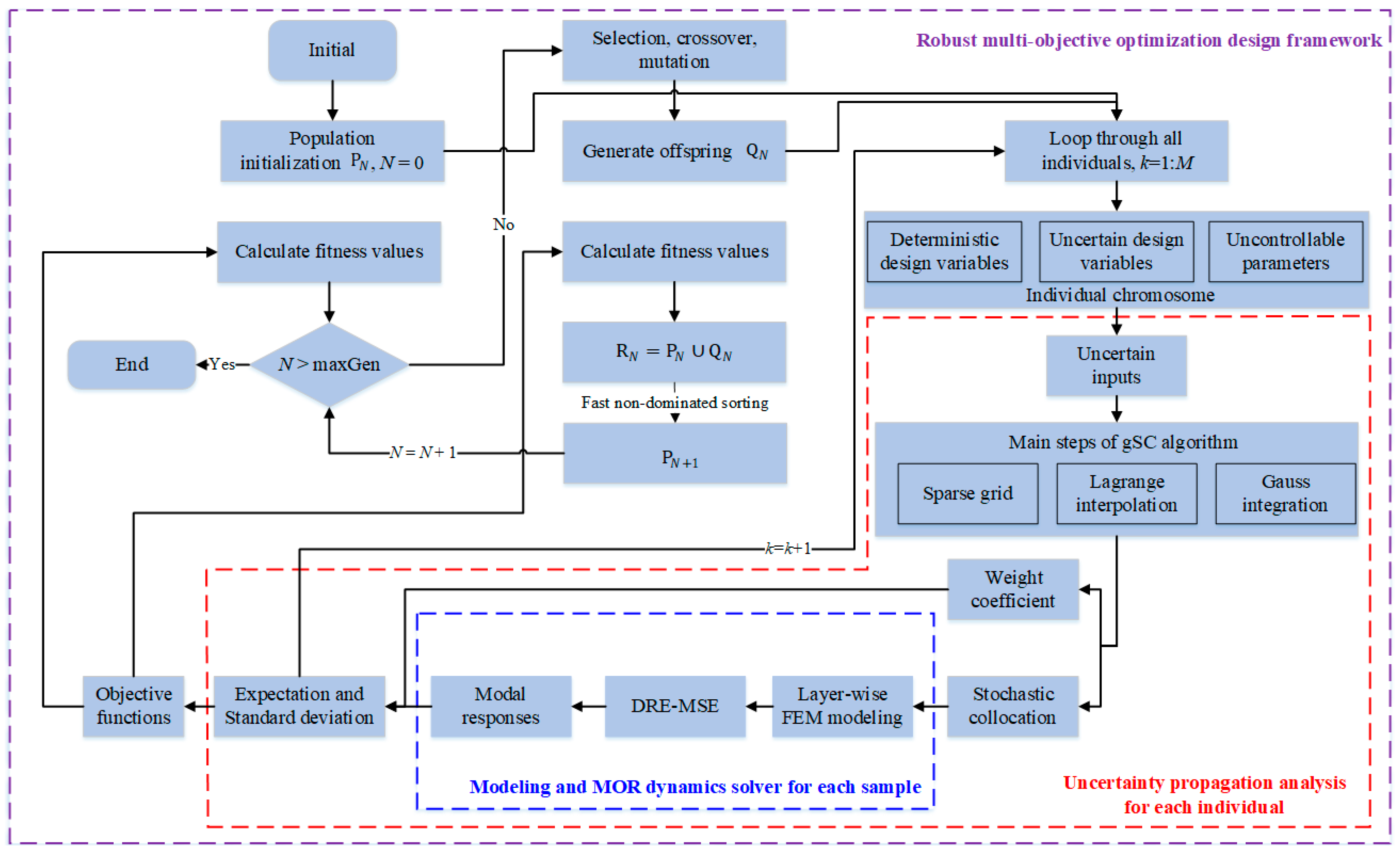
To efficiently solve the RDO problems for viscoelastic damped composite structures and ensure their effectiveness in engineering applications, this section integrates the advanced multi-objective genetic algorithm, NSGA-II, the projection-based MOR method, and the uncertainty propagation algorithms. This integration leads to the development of a high-performance, accurate, and stable multi-objective robust optimization design framework.

4.2.1. Definition and Coding of Variables

Viscoelastic damped composite structures exhibit significant design flexibility, characterized by numerous design variables such as the thickness of the damping layer, the type of damping material, the embedding position of the damping layer, and the angle of composite ply, as illustrated in Figure 3. The thickness of the viscoelastic damping layer can be determined based on design requirements and is typically treated as a continuous variable. Different viscoelastic materials possess distinct performance characteristics, making the selection of damping material a crucial discrete design variable. When only one layer of viscoelastic material is present, the damping layer is usually positioned in the middle (core layer). However, the optimal embedding position must be determined when multiple layers are involved. Additionally, the angle of composite ply significantly influences overall stiffness and damping performance. Generally, it is represented as discrete values at specific intervals. For example, with an interval of $15°$, the design variable for each ply includes the values $\left\{90°, \pm 75°, \pm 60°, \pm 45°, \pm 30°, \pm 15°, 0°\right\}$.

In RDO, the incorporation of uncertainty factors necessitates new definitions for variables. These include deterministic design variables $x_{i_1}$, uncertain design variables $u_{i_2}^0$, and uncontrollable parameters $w_{i_3}$, where $i_1=1,\dots ,n_1$, $i_2=1,\dots ,n_2$, $i_3=1,\dots ,n_3$ with $n_1,n_2,n_3\in {\mathbb{N}}^{+}$. The deterministic design variables $x_{i_1}$ are defined within the design interval $\left[x_{i_1}^{\mathrm{L}},x_{i_1}^{\mathrm{U}}\right]$ and remain constant once selected, with $x_{i_1}^{\mathrm{L}}$ and $x_{i_1}^{\mathrm{U}}$ representing the lower and upper bounds of this interval, respectively. The uncertain design variables $u_{i_2}^0$ vary within the interval $\left[u_{i_2}^{\mathrm{L}},u_{i_2}^{\mathrm{U}}\right]$ and are defined as the expected value ${\mu }_{i_2}$ of the random variable $U_{i_2}$, corresponding to the uncertain parameter $u_{i_2}$, such that $U_{i_2}~{\pi }_{u_{i_2}}\left(u_{i_2}\right)$ and $\mathbb{E}\left(U_{i_2}\right)={\mu }_{i_2}=u_{i_2}^0$. The uncontrollable parameters $w_{i_3}$ exist outside the design space but influence the outcomes of robust optimization, with their corresponding random variables denoted as $W_{i_3}$, satisfying $W_{i_3}~{\pi }_{w_{i_3}}\left(w_{i_3}\right)$. These new variable definitions are essential for RDO as they aid in the coding process of genetic algorithms applied to RDO:

• The deterministic design variables employ the same mixed coding as in the deterministic design framework;
• The uncertain design variables follow a continuous probability density distribution with a fixed Coefficient of Variation (CoV), where the expectation is encoded as real numbers within the design interval, and the standard deviation is calculated from the CoV;
• The uncontrollable parameters generally adhere to a fixed continuous probability density distribution, but may exhibit different continuous probability density distributions when correlated with deterministic design variables.

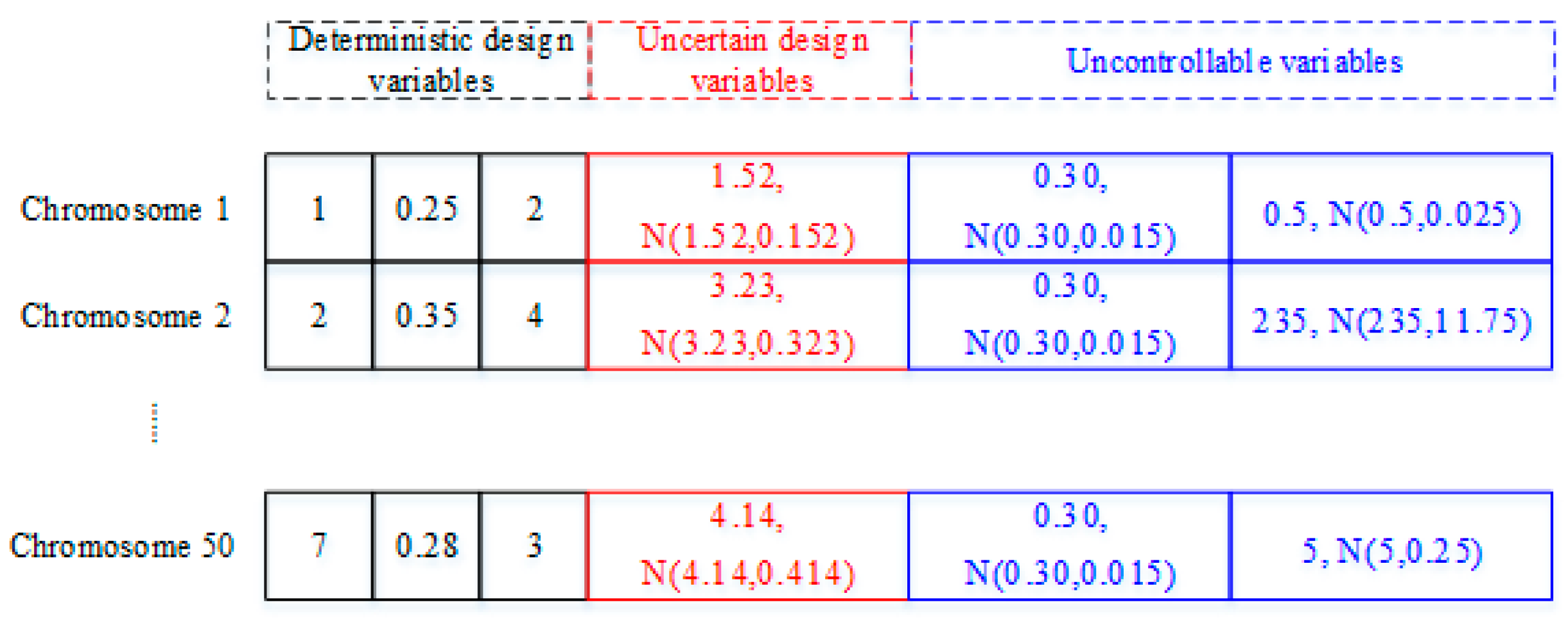
Figure 4 illustrates the composition of the initial population, comprising three deterministic design variables, one uncertain design variable, and two uncontrollable parameters. Each chromosome contains six genes: genes 1, 2, and 3 represent the mixed-coded deterministic design variables, consistent with the coding for design variables in deterministic optimization, which will not be elaborated further. Gene 4 is an uncertain design variable that is continuously encoded within the design interval $\left[1,5\right]$ and follows a normal probability density distribution with a CoV of 10% at each design point. For instance, gene 4 in chromosome 1 is $“1.52”$ drawn from$\mathrm{N}\left(1.52,0.152\right)$, in chromosome 2 is $“3.23”$ drawn from$\mathrm{N}\left(3.23,0.323\right)$, and in chromosome 3 is $“4.14”$ drawn from$\mathrm{N}\left(4.14,0.414\right)$. Gene 5 corresponds to an uncontrollable parameter that adheres to a fixed continuous probability density distribution. In chromosomes 1, 2, and 50, this gene is $“0.30”$ drawn from$\mathrm{N}\left(0.30,0.015\right)$. Gene 6 represents a different uncontrollable parameter that is correlated with gene 3 (assuming gene 3 represents the type of viscoelastic material and gene 6 denotes the modulus of that material). In chromosome 1, gene 6 (for 3M ISD-112 material) is $“0.5”$ drawn from $\mathrm{N}\left(0.5,0.025\right)$, in chromosome 2 (for PVB material) it is $“235”$ drawn from $\mathrm{N}\left(235,11.75\right)$, and in chromosome 3 (for GE SMRD material) it is $“5”$ drawn from $\mathrm{N}\left(5,0.25\right)$.

4.2.2. Robust Handling of Optimization Objectives and Constraints

The optimization design of viscoelastic damped composite structures primarily focuses on their load-bearing capacity and damping performance. Consequently, high stiffness, high strength, high damping, and lightweight characteristics are often regarded as desirable design objectives. In the context of specific structural design, these common optimization goals can be articulated as:

• Maximize modal natural frequency;
• Maximize modal damping ratio;
• Minimize structural mass.

However, due to the presence of uncertain design variables $u_{i_2}^0$ or uncontrollable parameters $w_{i_3}$, any objective function is no longer a deterministic real number but exhibits probabilistic fluctuations represented as the random variable $F\left(\mathit{x},{\mathit{u}}^0,\mathit{w}\right)$. The goal of RDO is to select appropriate nominal values for deterministic or uncertain design variables, ensuring that the random objective values optimize average performance while remaining insensitive to uncertainty factors. Thus, robustness handling of optimization objectives becomes the most critical aspect of RDO. Currently, two common methods for handling robustness in objective functions are defined by their mean and standard deviation. The first method treats the mean and standard deviation of the deterministic objective function as indicators of average performance and robustness, respectively, effectively doubling the number of objectives compared to the original deterministic optimization problem. However, an excessive number of optimization objectives can complicate the convergence of genetic algorithms and impact the final decision-making of designers. Therefore, the second method combines the mean and standard deviation of any deterministic objective function linearly, ensuring that the total number of objectives does not increase during optimization. This approach balances average performance and robustness for each objective without increasing their count. For bi-objective optimization, the objective functions processed in this manner can be expressed as:

$$\left\{\begin{array}{c}{\varphi }_1\left(\mathit{x},{\mathit{u}}^0,\mathit{w}\right)={\mu }_{F_1\left(\mathit{x},{\mathit{u}}^0,\mathit{w}\right)}+\lambda {\mathrm{\sigma }}_{F_1\left(\mathit{x},{\mathit{u}}^0,\mathit{w}\right)}\\ {\varphi }_2\left(\mathit{x},{\mathit{u}}^0,\mathit{w}\right)={\mu }_{F_2\left(\mathit{x},{\mathit{u}}^0,\mathit{w}\right)}+\lambda {\mathrm{\sigma }}_{F_2\left(\mathit{x},{\mathit{u}}^0,\mathit{w}\right)}\end{array}\right.$$

(32)

where $\mathit{x}$ is a vector containing $n_1$ deterministic design variables, $\mathit{x}={\left[x_1,x_2,\dots ,x_{n_1}\right]}^{\mathrm{T}}$, ${\mathit{u}}^0$ is a vector of $n_2$ uncertain design variables, ${\mathit{u}}^0={\left[u_1^0,u_2^0,\dots ,u_{n_2}^0\right]}^{\mathrm{T}}$, $\mathit{w}$ is a vector of $n_3$ uncontrollable parameters, $\mathit{w}={\left[w_1,w_2,\dots ,w_{n_3}\right]}^{\mathrm{T}}$, and $\lambda$ represents the preference factor for robustness handling (here, we set $\lambda =1)$. It is important to note that the standard deviation of objective functions is typically minimized. However, for certain objective functions where maximizing expected performance is desired, the negative or reciprocal of the objective function can be employed as a substitute. In this study, the reciprocal is utilized for the expected results related to natural frequency and damping ratio.

Constraints in design optimization ensure that the obtained optimal solution is physically feasible. The constraints fall into three categories: upper and lower limits on design variables, inequality constraints, and equality constraints. Together, they define the feasible region of solutions. In this study, these constraints in RDO are simplified using nominal values.

4.2.3. Robust Multi-Objective Optimization Design Framework

Based on the above discussion, we summarize the robust multi-objective optimization design framework for viscoelastic damped composite structures, as illustrated in Figure 5.

5. Examples and Results

This section includes four examples: the first and second examples validate the effectiveness of the projection-based MOR algorithm and gSC algorithm, respectively, while the third and fourth examples apply the robust multi-objective optimization design framework to both a simple and a complex viscoelastic damped structure. It should be noted that all calculations in this study were conducted on a computer equipped with a quad-core Intel i7-6700 processor (3.40 GHz) and 16.0 GB of RAM.

5.1. Four-Sided Simply Supported Sandwich Damped Panel

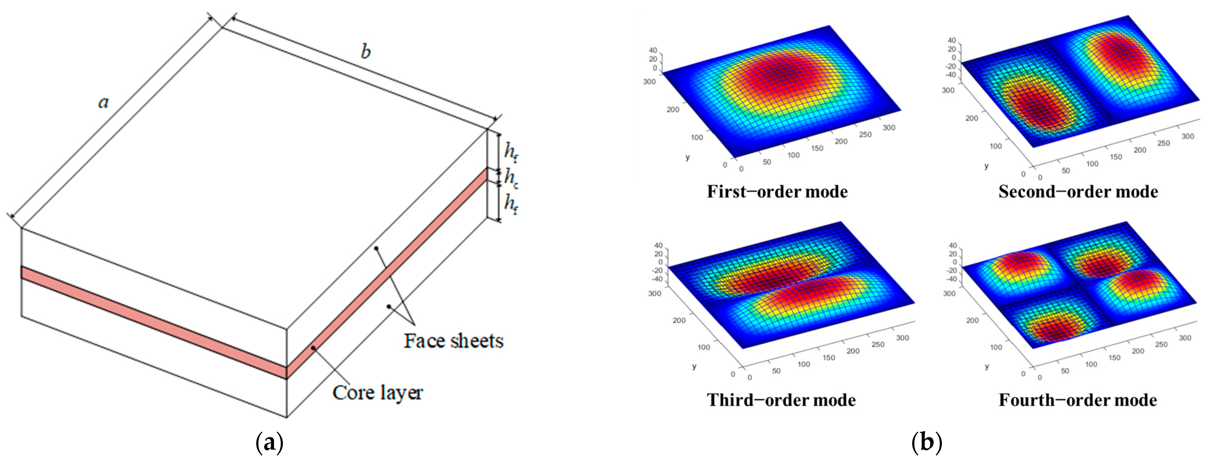
To validate the proposed model reduction method, a four-sided simply supported (SSSS) sandwich damped panel is analyzed, as illustrated in Figure 6a. The in-plane dimensions are set as a = 348 mm and b = 304.8 mm, while the thickness dimensions are $h_{\mathrm{f}}=0.762 \mathrm{m}\mathrm{m}$ for the face sheets and $h_{\mathrm{c}}=0.254 \mathrm{m}\mathrm{m}$ for the core layer. The material parameters for the elastic panel are: $E_{\mathrm{f}}=68.9\mathrm{GPa}$, ${\nu }_{\mathrm{f}}=0.3$, ${\rho }_{\mathrm{f}}=2740\mathrm{kg}/{\mathrm{m}}^3$. The core material comprises six frequency-dependent viscoelastic damping materials, as listed in Table 1. Figure 6b presents the first four modes for the undamped system, which will be tracked as modal vectors by the proposed MOR methods.

Initially, four methods—namely I-IRA, MSE, E-MSE, and DRE-MSE—are utilized to compute the first four modal frequencies and damping ratios of the structure. For the I-IRA and DRE-MSE methods, which automatically iterate based on specified convergence tolerances, a convergence tolerance of 10⁻² is employed. Conversely, the MSE and E-MSE methods focus exclusively on the number of retained modal vectors, with the MSE method utilizing four undamped modal vectors and the E-MSE method employing eight. The results and computational costs derived from the I-IRA method are taken as the reference solution to evaluate the computational accuracy and efficiency of the MSE, E-MSE, and DRE-MSE methods. The structural mesh size is established as 32 × 28.

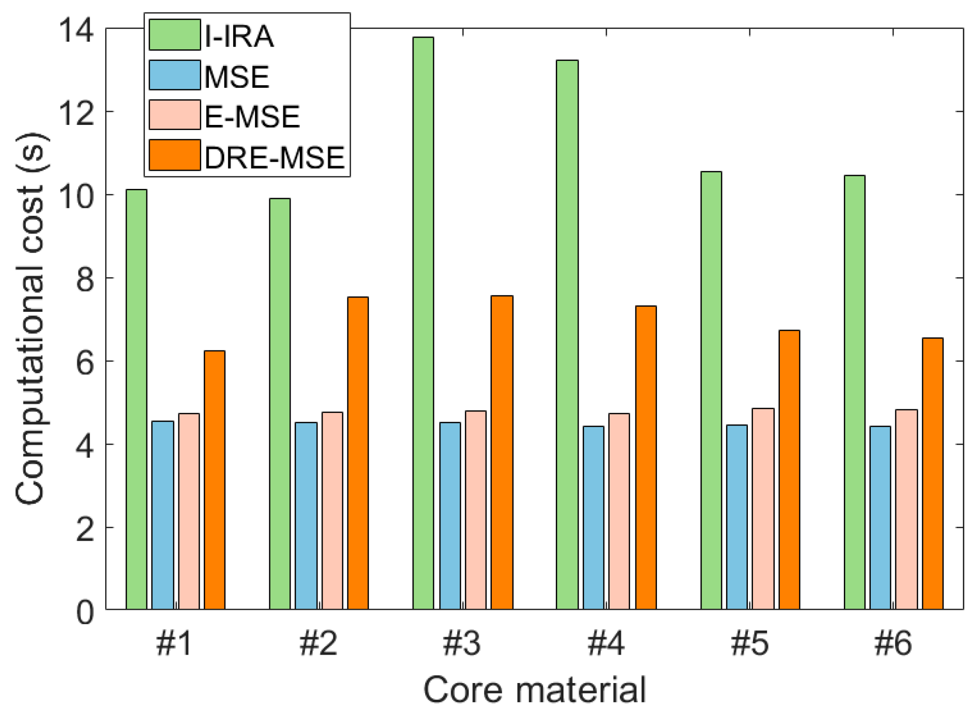
Figure 7 outlines the computational costs associated with four methods applied to six different frequency-dependent viscoelastic core sandwiched structures. Among these, the I-IRA method is the most computationally intensive, requiring 10.12, 10.17, 13.45, 12.39, 10.25, and 10.76 s for structures using materials #1 to #6, respectively. In contrast, the MSE and E-MSE methods demonstrate substantially lower computational demands. Specifically, the E-MSE method takes 4.72, 4.75, 4.80, 4.72, 4.85, and 4.83 s for the same set of materials, while the MSE method shows similar efficiency, requiring 4.55, 4.51, 4.52, 4.42, 4.46, and 4.42 s. The DRE-MSE method, although slightly more expensive than the MSE and E-MSE methods, remains considerably lower than the I-IRA method, with times of 6.59, 7.73, 8.24, 7.67, 7.02, and 6.94 s for materials #1 to #6. In terms of average computational time, the MSE and E-MSE methods achieve reductions of 60% and 57%, respectively, compared to the I-IRA method, while the DRE-MSE method reduces computation time by 34%.

Table 2. First four modal frequencies and damping ratios of viscoelastic sandwich panels with six different frequency-dependent core materials: A comparative analysis of four nonlinear eigenvalue solution methods.

Viscoelastic Materials	I-IRA		MSE		E-MSE		DRE-MSE
	${\mathit{f}}_{\mathit{r}}$ (Hz)	${\mathit{\eta }}_{\mathit{r}}$	${\mathit{f}}_{\mathit{r}}$ (Hz)	${\mathit{\eta }}_{\mathit{r}}$	${\mathit{f}}_{\mathit{r}}$ (Hz)	${\mathit{\eta }}_{\mathit{r}}$	${\mathit{f}}_{\mathit{r}}$ (Hz)	${\mathit{\eta }}_{\mathit{r}}$
3M ISD−112	53.71	0.218	52.58	0.274	53.71	0.217	53.71	0.218
	110.46	0.283	108.46	0.353	110.44	0.282	110.46	0.283
	126.67	0.294	124.49	0.361	126.64	0.294	126.67	0.294
	176.79	0.302	173.89	0.367	176.77	0.302	176.79	0.302
PVB	82.74	5.581 × 10−3	513.02	0.140	167.94	0.142	82.74	5.579 × 10−3
	190.17	5.767 × 10−3	980.12	0.125	353.18	0.118	190.18	5.766 × 10−3
	223.25	5.570 × 10−3	1095.84	0.122	398.60	0.112	223.25	5.557 × 10−3
	326.48	7.720 × 10−3	1396.99	0.117	544.43	0.103	326.48	7.750 × 10−3
ZN−1	61.63	0.288	58.21	0.562	61.51	0.288	61.63	0.288
	132.17	0.378	125.58	0.707	132.69	0.381	132.17	0.378
	152.74	0.402	144.88	0.727	152.18	0.406	152.74	0.402
	214.16	0.423	203.42	0.746	213.46	0.425	214.16	0.424
DM 9740	79.49	0.079	114.64	1.179	79.91	0.210	79.37	0.078
	184.56	0.098	264.22	2.026	184.26	0.239	184.54	0.098
	217.87	0.099	304.66	2.285	217.07	0.209	217.84	0.099
	319.57	0.126	407.60	2.911	312.76	0.397	319.40	0.125
GE SMRD	80.79	0.036	106.08	0.496	81.41	0.073	80.77	0.034
	186.41	0.034	319.10	0.554	189.16	0.079	186.39	0.034
	219.12	0.032	396.28	0.546	221.65	0.067	219.10	0.033
	319.93	0.039	622.09	0.510	329.68	0.112	319.94	0.042
EAR C−1002	57.22	0.069	57.18	0.080	57.18	0.080	57.18	0.080
	114.85	0.106	114.75	0.120	114.75	0.120	114.75	0.120
	131.19	0.113	131.07	0.127	131.07	0.127	131.07	0.127
	180.81	0.119	180.64	0.132	180.64	0.132	180.64	0.132

presents the results of the first four modal natural frequencies and damping ratios calculated using four methods for six different frequency-dependent viscoelastic material sandwich structures. It can be observed that the MSE method yields relatively accurate natural frequency results for cases #1 and #6, although the errors in the modal damping ratios are substantial yet acceptable. For case #3, the natural frequency deviates somewhat from the reference solution, and the error in the modal damping ratio is significant. In cases #2, #4, and #5, both the natural frequencies and modal damping ratios diverge considerably from the reference solution.

The E-MSE method achieves highly accurate modal natural frequency and damping ratio results for cases #1, #3, and #6. In cases #4 and #5, the modal natural frequency results are acceptable, but the errors in the modal damping ratios are quite large. For case #2, both the modal natural frequency and damping ratio exhibit substantial deviations. In contrast, the DRE-MSE method demonstrates complete consistency with the reference solutions for both the modal natural frequencies and damping ratios across all six viscoelastic material scenarios.

In summary, the MSE method struggles to accurately calculate the natural frequencies in most cases and fails to do so for all modal damping ratios. The E-MSE method is applicable only to cases #1, #3, and #6, which may be related to the relatively low storage moduli of the viscoelastic materials depicted in Figure 1. The DRE-MSE method, on the other hand, proves suitable for all scenarios, meeting accuracy requirements while maintaining high computational efficiency.

A further investigation was carried out to assess the sensitivity of the computational efficiency of the proposed DRE-MSE method concerning DoFs and required accuracy. The analysis still focused on the first four modal natural frequencies and damping ratios of structures incorporating six different viscoelastic materials. To enhance clarity and conciseness, only the average errors associated with these frequencies and damping ratios are presented.

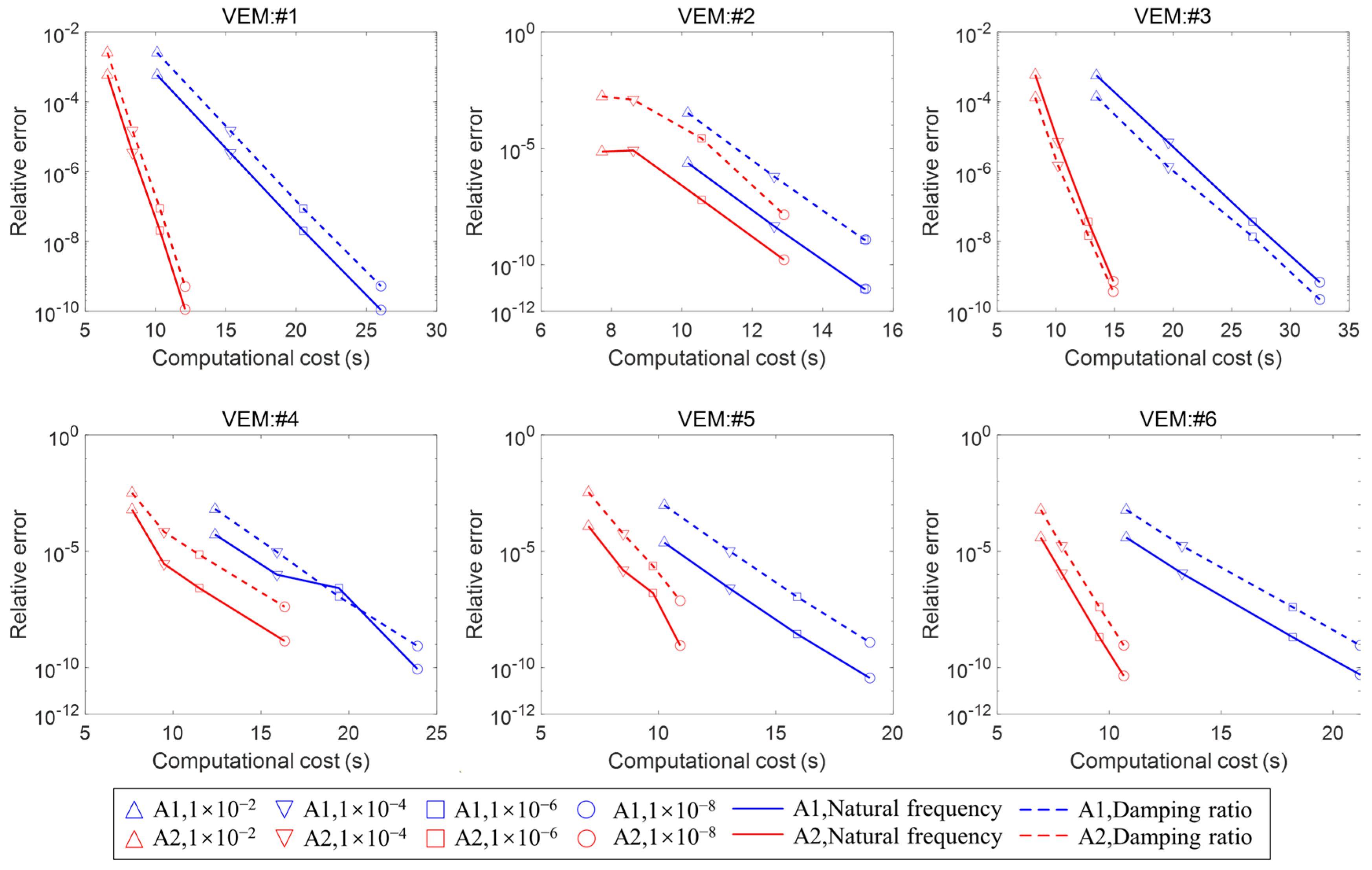
Figure 8 depicts the relationship between the actual average relative errors and computation times obtained using the DRE-MSE method under different convergence tolerance requirements ${\epsilon }_{\mathrm{t}}$ (specifically 1 × 10⁻², 1 × 10⁻⁴, 1 × 10⁻⁶, and 1 × 10⁻⁸) for a mesh size of 32 × 28 (9570 DoFs). Additionally, the corresponding results from the I-IRA method are included for comparative reference. It is essential to clarify the legend. Among these, A1 (blue) and A2 (red) represent the I-IRA and DRE-MSE methods, respectively, with different markers indicating the various convergence tolerances. Solid lines denote the average error data for modal natural frequencies, while dashed lines represent the average error data for modal damping ratios. The results reveal several key insights. On one hand, for both algorithms, the actual errors decrease as the convergence tolerance ${\epsilon }_{\mathrm{t}}$ is reduced, indicating that the control parameter ${\epsilon }_{\mathrm{t}}$ can effectively adjust the accuracy of the predictions. On the other hand, in all cases, the DRE-MSE method consistently requires less computation time than the I-IRA method. However, for high accuracy requirements, such as in cases #2, #3, and #5 at ${\epsilon }_{\mathrm{t}}$ values of “1 × 10⁻⁶” and “1 × 10⁻⁸”, the actual computational accuracy of the DRE-MSE method is slightly lower than that of the I-IRA method. Nevertheless, this issue may not be critical in practical engineering applications, as achieving such high precision in modal results is often unnecessary. Overall, the DRE-MSE method demonstrates significantly higher computational efficiency compared to the I-IRA method. At larger ${\epsilon }_{\mathrm{t}}$ values, which are typically required in actual situations, the computational accuracies of both methods are quite similar, with actual errors remaining below the convergence tolerance. However, at very small ${\epsilon }_{\mathrm{t}}$ values, the accuracy of the DRE-MSE method is relatively lower. Figure 9 shows the relationship between the relative errors and computation times for six sandwich structures (37,050 DoFs) under different ${\epsilon }_{\mathrm{t}}$ values. Additionally, it is evident that as the DoFs increase, the computation times for both methods exhibit a significant rise. For the average computation times of the six different viscoelastic damped composite structures, the I-IRA method shows calculation times of 11.19, 14.95, 19.33, and 22.98 s under progressively higher error requirements for 9570 DoF structures, while the DRE-MSE method requires averages of 7.36, 8.84, 10.74, and 12.97 s, resulting in cost reductions of 34%, 41%, 44%, and 43%, respectively, compared to the I-IRA method. In contrast, for 37,050 DoF structures, the I-IRA method records computation times of 51.44, 71.19, 93.10, and 111.76 s under the same error requirements, while the DRE-MSE method averages 31.93, 39.52, 48.75, and 60.80 s, yielding reductions of 38%, 44%, 47%, and 45% compared to the I-IRA method. In addition, an interesting phenomenon is observed: in all cases except VEM #3, the predicted frequency is consistently more accurate than the predicted damping ratio. This is because the frequency can be predicted very precisely even when projected with nominal modes, and the constantly updated projection basis will make it even more accurate. However, the accuracy of the damping result must be progressively enhanced through continuous (residual term) enhanced projection. Of course, this update of the projection basis is not mechanically accurate, and VEM #3 can be considered an occasional exception. That is, the last update of the projection basis before convergence is very good for damping prediction.

In summary, the proposed DRE-MSE method effectively addresses the nonlinear eigenvalue problems of various viscoelastic damped composite structures while maintaining computational accuracy. Furthermore, the DRE-MSE method demonstrates robustness regarding computational cost improvements, showing insensitivity to the set error convergence limits and the scale of structural degrees of freedom.

5.2. Four-Sided Fixed Viscoelastic Damped Laminated Plate

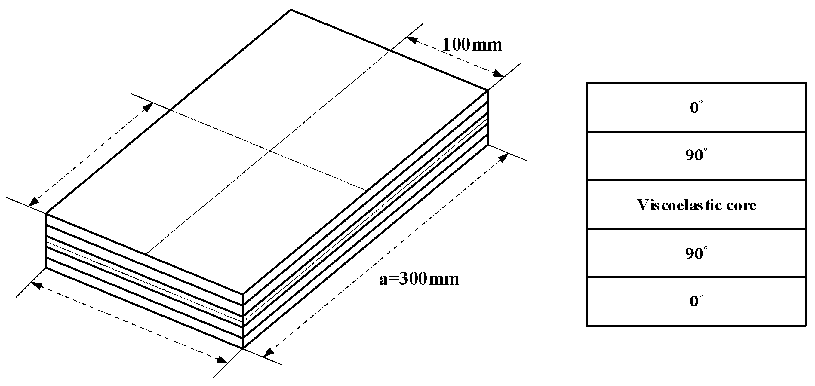
As shown in Figure 10, a four-sided fixed viscoelastic damped laminated plate is considered, measuring 300 mm in length and 200 mm in width, with boundary conditions fixed on all four sides. The laminated structure consists of five layers in the thickness direction, with the stacking sequence of [0°/90°/core/90°/0°]. Each layer has a thickness of 0.2 mm. The fiber-reinforced laminated layers are made of carbon/epoxy material [58], while the core layer is composed of material #1 (3M ISD-112) from Table 1. In this analysis, uncertainty parameters include not only the core layer thickness and the mechanical properties of the viscoelastic material but also the mechanical properties of the composite material, as detailed in

Table 3. Uncertain parameters for the viscoelastic damped laminated plate.

Type	Parameters	Random Distribution	Sources
Core layer	$h_{\mathrm{c}}$ (mm)	$h_{\mathrm{c}}~\mathrm{N}(0.127,{0.00635}^2)$	Assumed
	$G_0$ (MPa)	$G_0~\mathrm{N}\left(0.5,{0.025}^2\right)$	Assumed
Fiber-reinforced laminated layers	$E_{11}$ (GPa)	$E_{11}~\mathrm{Wb}\left(158.9,20.7\right)$	[58]
	$E_{22}$ (GPa)	$E_{22}~\mathrm{Wb}\left(9.0,14.4\right)$
	$G_{12}$ (GPa)	$\mathrm{l}\mathrm{n}{G}_{12}~\mathrm{N}\left(1.49,{0.09}^2\right)$
	$G_{13}$ (GPa)	$\mathrm{l}\mathrm{n}{G}_{13}~\mathrm{N}\left(1.49,{0.09}^2\right)$
	$G_{23}$ (GPa)	$\mathrm{l}\mathrm{n}{G}_{23}~\mathrm{N}\left(1.356,{0.1}^2\right)$

.

Before UP analysis, a deterministic modal analysis was initially conducted using the nominal values of the uncertain parameters. The convergence tolerance requirement ${\epsilon }_{\mathrm{t}}$ for the DRE-MSE algorithm was set at 1 × 10⁻⁴, and a mesh convergence analysis confirmed that a mesh size of 24 × 16 fulfilled the computational requirements, yielding a total of 4250 DoFs. To validate the effectiveness of the gSC method, eight sets of MCS will be performed for comparison, with sample sizes of 10, 50, 100, 500, 1000, 5000, 10,000, and 100,000, where the results from the 100,000-sample simulation will serve as the reference solution. To analyze the convergence of the gSC method, UP analysis will employ four interpolation levels, denoted as $q=1,2,3 \mathrm{a}\mathrm{n}\mathrm{d} 4$. The corresponding sample sizes are 15, 118, 654, and 2877 in this seven-dimensional UP problem.

Figure 11 illustrates the convergence results for the natural frequencies. At $q=1,$ with a total of $m=15$ nodes, the expectations obtained via the gSC method for the first four modes converged to values of 1.72 × 10⁻⁵, 2.54 × 10⁻⁵, 8.61 × 10⁻⁷, and 7.84 × 10⁻⁶, while the corresponding standard deviations converged to 2.40 × 10⁻³, 2.27 × 10⁻³, 5.00 × 10⁻⁴, and 1.07 × 10⁻³. In contrast, the expectations and standard deviations obtained via the MCS were approximately 1 to 2 orders of magnitude higher at $m=\mathrm{10,000}$. For the damping ratios, the expectations and standard deviations obtained from the MCS at $m=\mathrm{10,000}$ also exhibited approximately 1 order of magnitude higher levels. Overall, the gSC method demonstrated a significantly faster convergence rate compared to MCS, even in a scenario characterized by seven random dimensions.

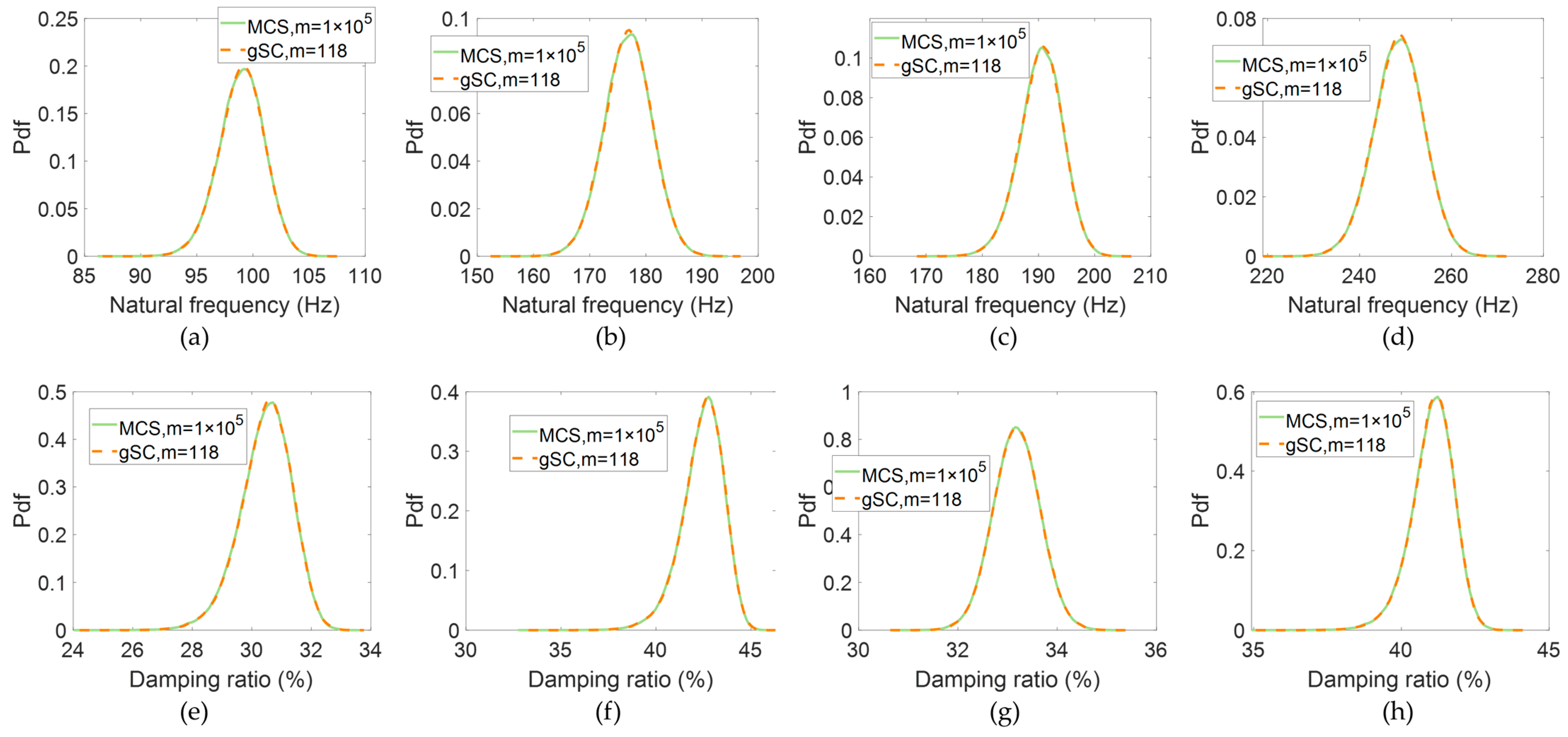
Notably, the computational results had already converged when $q$ was iterated to 2, thereby establishing a surrogate requiring only 118 samples via the gSC method. The desired PDFs for responses of natural frequency and damping ratio can be derived from a sufficient number of samples. Figure 12 presents these PDF results obtained using both the MCS and gSC methods. The close agreement between the results from both methods reinforces the validity of the gSC method as a reliable tool for UP analysis of viscoelastic damped composite structures.

5.3. Robust Design Optimization of a Cantilever Viscoelastic Sandwich Beam Plate

This example explores the optimal design of a cantilever viscoelastic sandwich beam plate, concentrating on the first mode response. As illustrated in Figure 13, the cantilever viscoelastic sandwich beam plate consists of two elastic face sheets and a soft core layer. The initial design specifies the in-plane geometric dimensions as follows: length $l=177.8 \mathrm{m}\mathrm{m}$, width $w=12.7 \mathrm{m}\mathrm{m}$, with thickness $h_{\mathrm{f}}=1.524 \mathrm{m}\mathrm{m}$ and $h_{\mathrm{c}}=0.127 \mathrm{m}\mathrm{m}$. The material parameters for the elastic face sheets are: Young’s modulus $E_{\mathrm{f}}=69 \mathrm{G}\mathrm{P}\mathrm{a}$, Poisson’s ratio $v_{\mathrm{f}}=0.3$, and density ${\rho }_{\mathrm{f}}=2766 \mathrm{k}\mathrm{g}/{\mathrm{m}}^3$. The core material employed is 3M ISD-112. The primary objective of this example is to evaluate the distinctions between deterministic and robust optimization designs while evaluating the effects of various sources of uncertainty on the optimization outcomes. This will provide insights into the implications of neglecting certain uncertainty factors. The DRE-MSE method is used to evaluate the fundamental modal natural frequencies and damping ratios, with an error tolerance set to ${\epsilon }_{\mathrm{t}}=1 \times {10}^{-4}$.

In the deterministic scenario, the core layer thickness $h_{\mathrm{c}}$ and the elastic layer thickness $h_{\mathrm{f}}$ are defined as design variables, denoted as $x_1$ and $x_2$, with respective value ranges of [0.05 mm, 8 mm] and [0.05 mm, 2 mm]. The mathematical formulation for this deterministic optimization is:

$$\left\{\begin{array}{c}\mathrm{find} \mathit{x} \\ \mathrm{m}\mathrm{i}\mathrm{n}\mathrm{i}\mathrm{m}\mathrm{i}\mathrm{z}\mathrm{e} \left\{F_1\left(\mathit{x}\right),F_2\left(\mathit{x}\right)\right\} \\ \mathrm{s}\mathrm{u}\mathrm{b}\mathrm{j}\mathrm{e}\mathrm{c}\mathrm{t} \mathrm{t}\mathrm{o} \mathit{x}={\left[x_1,x_2\right]}^{\mathrm{T}} \\ 0.05\le x_1\le 8 \left(\mathrm{m}\mathrm{m}\right) \\ 0.05\le x_2\le 2 \left(\mathrm{m}\mathrm{m}\right) \end{array}\right.$$

(33)

For uncertain scenarios, three cases are analyzed. Case 1 studies the uncertainty of the viscoelastic material alone. Here, both the core layer thickness $h_{\mathrm{c}}$ and the elastic layer thickness $h_{\mathrm{f}}$ remain deterministic design variables, represented as $x_1$ and $x_2$, with value ranges as established in the deterministic scenario. The viscoelastic material modulus $G_0$ is treated as an uncontrollable parameter, designated as $w_1$. The corresponding random variable $W_1$ follows a normal distribution, $W_1~\mathrm{N}(0.5,{0.025}^2)$, with units in MPa. The optimization formulation is:

$$\left\{\begin{array}{c}\mathrm{find} \mathit{x} \\ \mathrm{m}\mathrm{i}\mathrm{n}\mathrm{i}\mathrm{m}\mathrm{i}\mathrm{z}\mathrm{e} \left\{{\varphi }_1\left(\mathit{x},\mathit{w}\right),{\varphi }_2\left(\mathit{x},\mathit{w}\right)\right\} \\ \mathrm{s}\mathrm{u}\mathrm{b}\mathrm{j}\mathrm{e}\mathrm{c}\mathrm{t} \mathrm{t}\mathrm{o} \mathit{x}={\left[x_1,x_2\right]}^{\mathrm{T}}, \mathit{w}={\left[w_1\right]}^{\mathrm{T}} \\ 0.05\le x_1\le 8 \left(\mathrm{m}\mathrm{m}\right) \\ 0.05\le x_2\le 2 \left(\mathrm{m}\mathrm{m}\right) \\ W_1~N\left(0.5,{0.025}^2\right) \left(\mathrm{M}\mathrm{P}\mathrm{a}\right)\end{array}\right.$$

(34)

Case 2 focuses on the uncertainty of the core layer thickness. In this scenario, the elastic layer thickness $h_{\mathrm{f}}$ continues to be a deterministic design variable, denoted as $x_1$, with the same value range as in the deterministic case. In contrast, the core layer thickness $h_{\mathrm{c}}$ is treated as an uncertain design variable, defined as $u_1^0$, with a value range of [0.05 mm, 8 mm]. The random variable $U_1$ is assumed to follow a normal distribution with a CoV of 5%. The optimization formulation is stated as:

$$\left\{\begin{array}{c}\mathrm{find} \mathit{x} \mathrm{and} {\mathit{u}}^0 \\ \mathrm{m}\mathrm{i}\mathrm{n}\mathrm{i}\mathrm{m}\mathrm{i}\mathrm{z}\mathrm{e} \left\{{\varphi }_1\left(\mathit{x},{\mathit{u}}^0\right),{\varphi }_2\left(\mathit{x},{\mathit{u}}^0\right)\right\} \\ \mathrm{s}\mathrm{u}\mathrm{b}\mathrm{j}\mathrm{e}\mathrm{c}\mathrm{t} \mathrm{t}\mathrm{o} \mathit{x}={\left[x_1\right]}^{\mathrm{T}}, {\mathit{u}}^0={\left[u_1^0\right]}^{\mathrm{T}} \\ 0.05\le x_1\le 8 \left(\mathrm{m}\mathrm{m}\right) \\ 0.05\le x_2\le 2 \left(\mathrm{m}\mathrm{m}\right) \\ U_1~N\left({\mu }_1,{{\sigma }_1}^2\right),\mathbb{E}\left(U_1\right)={\mu }_1=u_1^0\\ {\mathrm{C}\mathrm{o}\mathrm{V}}_{U_1}=\left({\sigma }_1/u_1^0\right)\times 100\%=5\%\end{array}\right.$$

(35)

In Case 3, both the uncertainties related to the viscoelastic material and the core layer thickness are accounted for. The elastic layer thickness $h_{\mathrm{f}}$ remains a deterministic design variable, while the core layer thickness $h_{\mathrm{c}}$ and the viscoelastic material modulus $G_0$ are treated as the uncertain design variable and the uncontrollable parameter, respectively. The definitions, value ranges, and probability density distributions for the random variables remain consistent with the previous cases. The optimization formulation is expressed as:

$$\left\{\begin{array}{c}\mathrm{find} \mathit{x} \mathrm{and} {\mathit{u}}^0 \\ \mathrm{m}\mathrm{i}\mathrm{n}\mathrm{i}\mathrm{m}\mathrm{i}\mathrm{z}\mathrm{e} \left\{{\varphi }_1\left(\mathit{x},{\mathit{u}}^0,\mathit{w}\right),{\varphi }_2\left(\mathit{x},{\mathit{u}}^0,\mathit{w}\right)\right\} \\ \mathrm{s}\mathrm{u}\mathrm{b}\mathrm{j}\mathrm{e}\mathrm{c}\mathrm{t} \mathrm{t}\mathrm{o} \mathit{x}={\left[x_1\right]}^{\mathrm{T}}, {\mathit{u}}^0={\left[u_1^0\right]}^{\mathrm{T}}, \mathit{w}={\left[w_1\right]}^{\mathrm{T}} \\ 0.05\le x_1\le 8 \left(\mathrm{m}\mathrm{m}\right) \\ 0.05\le x_2\le 2 \left(\mathrm{m}\mathrm{m}\right) \\ U_1~N\left({\mu }_1,{{\sigma }_1}^2\right),\mathbb{E}\left(U_1\right)={\mu }_1=u_1^0\\ {\mathrm{C}\mathrm{o}\mathrm{V}}_{U_1}=\left({\sigma }_1/u_1^0\right)\times 100\%=5\%\\ W_1~N\left(0.5,{0.025}^2\right) \left(\mathrm{M}\mathrm{P}\mathrm{a}\right)\end{array}\right.$$

(36)

Finally,

Table 4. Variable settings for both the deterministic design and three RDO cases.

Scenario	Deterministic Design Variable	Uncertain Design Variable	Uncontrollable Parameter
Deterministic design	Core and elastic layer thickness, $x_1$ and $x_2$	−	−
RDO case 1	Core and elastic layer thickness, $x_1$ and $x_2$	−	Viscoelastic material modulus, $w_1$
RDO case 2	Elastic layer thickness, $x_1$	Core layer thickness, $u_1^0$	−
RDO case 3	Elastic layer thickness, $x_1$	Core layer thickness, $u_1^0$	Viscoelastic material modulus, $w_1$

summarizes the variable settings for both the deterministic optimization design and the three robust optimization design cases, offering clarity on the characteristics of the design variables in each scenario.

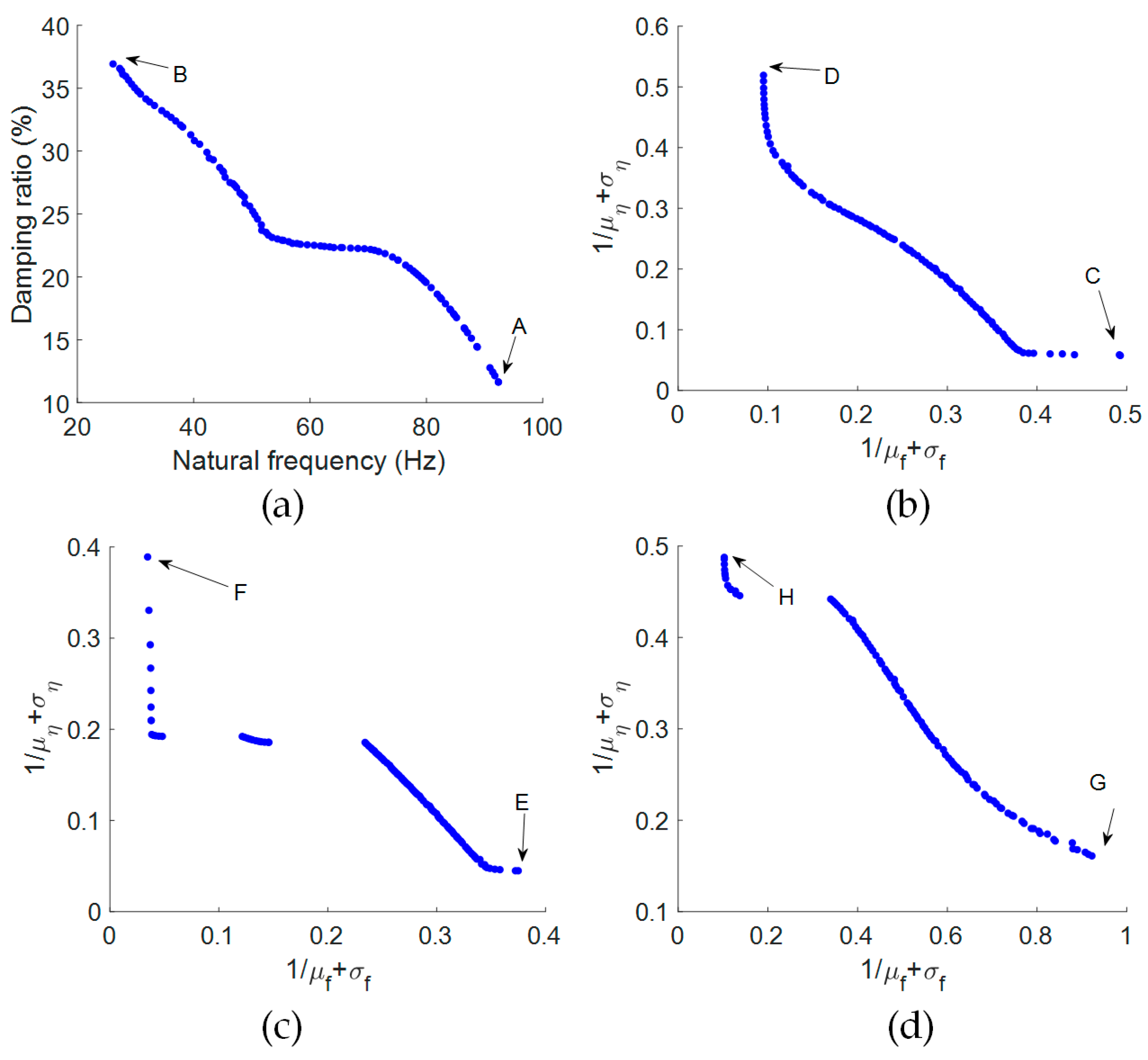
Figure 14 illustrates the convergence of Pareto optimal solutions for deterministic optimization design and three RDO cases (50 generations). For further analysis, we have labeled the maximum first natural frequency in the deterministic optimization design as A and the maximum first damping ratio as B in Figure 14a. In Figure 14b, the minimum robustness objective corresponding to the first damping ratio in RDO case 1 is marked as C, while the minimum robustness objective corresponding to the first natural frequency is labeled as D. Figure 14c marks the minimum robustness objective for the first damping ratio in RDO case 2 as E, and the corresponding minimum for the first natural frequency as F. Finally, in Figure 14d, the minimum robustness objective corresponding to the first damping ratio in RDO case 3 is denoted as G, with the corresponding minimum for the first natural frequency marked as H.

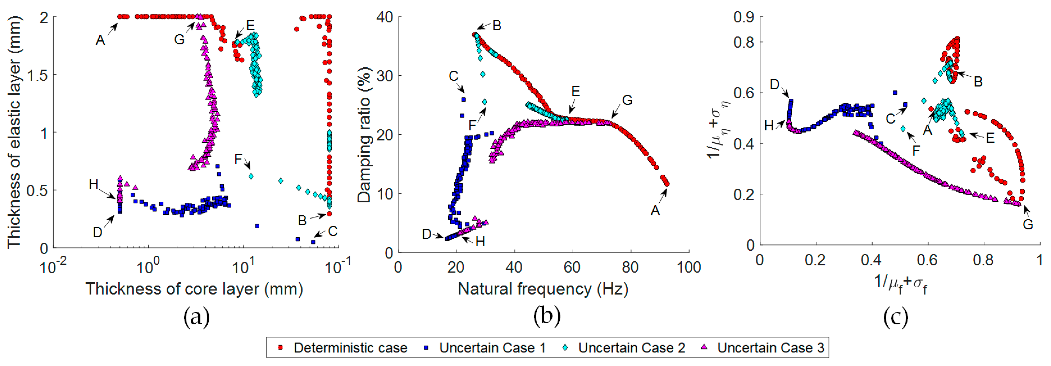
To comprehensively compare the differences between deterministic optimization design and RDO, as well as to analyze the impacts of omitting certain uncertainty factors, we conducted a series of simulation experiments using the 100 population individuals from the 50th generation. Initially, the converged individuals from the three RDO cases were employed in deterministic modal analysis to derive their natural frequencies and damping ratios under deterministic conditions. Subsequently, the converged individuals from the deterministic optimization design and the RDO cases 1 and 2 were utilized for UP analysis, specifically focusing on the uncertain input in the third case, which represents a real-world scenario. Following the application of robustness treatment, we identified the robustness objectives for these individuals within the context of the RDO case 3.

Figure 15 illustrates the optimal population individuals and subsequent simulation results for both the deterministic optimization design and the three RDO cases. Specifically, Figure 15a presents the design space corresponding to the optimal solutions of the four scenarios. Figure 15b depicts the deterministic solutions derived from these design spaces under deterministic conditions. Figure 15c shows the uncertainty solutions for these design spaces in the context of RDO case 3. The analysis reveals significant differences between deterministic optimization design and RDO. Moreover, the extent of uncertainty factors considered plays a crucial role in influencing the optimization results. The deterministic optimization design proves optimal only in deterministic scenarios. However, it performs markedly worse under uncertain conditions compared to RDO, which effectively accounts for uncertainty factors. Consequently, the more thoroughly uncertainty factors are integrated into the design process, the more robust the performance of the resulting optimization solutions becomes.

Table 5. Results of deterministic and three RDO cases for design scheme A−F.

Scheme	Design Variable		Deterministic Case		RDO Case 1		RDO Case 2		RDO Case 3
	${\mathit{h}}_{\mathbf{c}}$ (mm)	${\mathit{h}}_{\mathit{f}}$ (mm)	$\mathit{f}$ (Hz)	$\mathit{\eta }$ (%)	${\mathit{\varphi }}_1$	${\mathit{\varphi }}_2$	${\mathit{\varphi }}_1$	${\mathit{\varphi }}_2$	${\mathit{\varphi }}_1$	${\mathit{\varphi }}_2$
A	0.05	2.00	92.37	11.64	−	−	−	−	0.61	0.54
B	8.00	0.29	26.13	36.93	−	−	−	−	0.68	0.68
C	5.40	0.05	22.37	25.94	0.49	0.06	−	−	0.52	0.55
D	0.05	0.31	16.69	2.32	0.10	0.52	−	−	0.11	0.57
E	0.84	1.78	57.93	22.52	−	−	0.37	0.05	0.72	0.44
F	1.20	0.62	29.64	25.55	−	−	0.03	0.39	0.51	0.46
G	0.33	2.00	72.57	21.83	−	−	−	−	0.92	0.16
H	0.05	0.40	20.96	3.22	−	−	−	−	0.10	0.49

presents the deterministic results alongside three sets of uncertainty results for design schemes A–F.

5.4. Robust Design Optimization of Damping Brackets for Infrared Devices

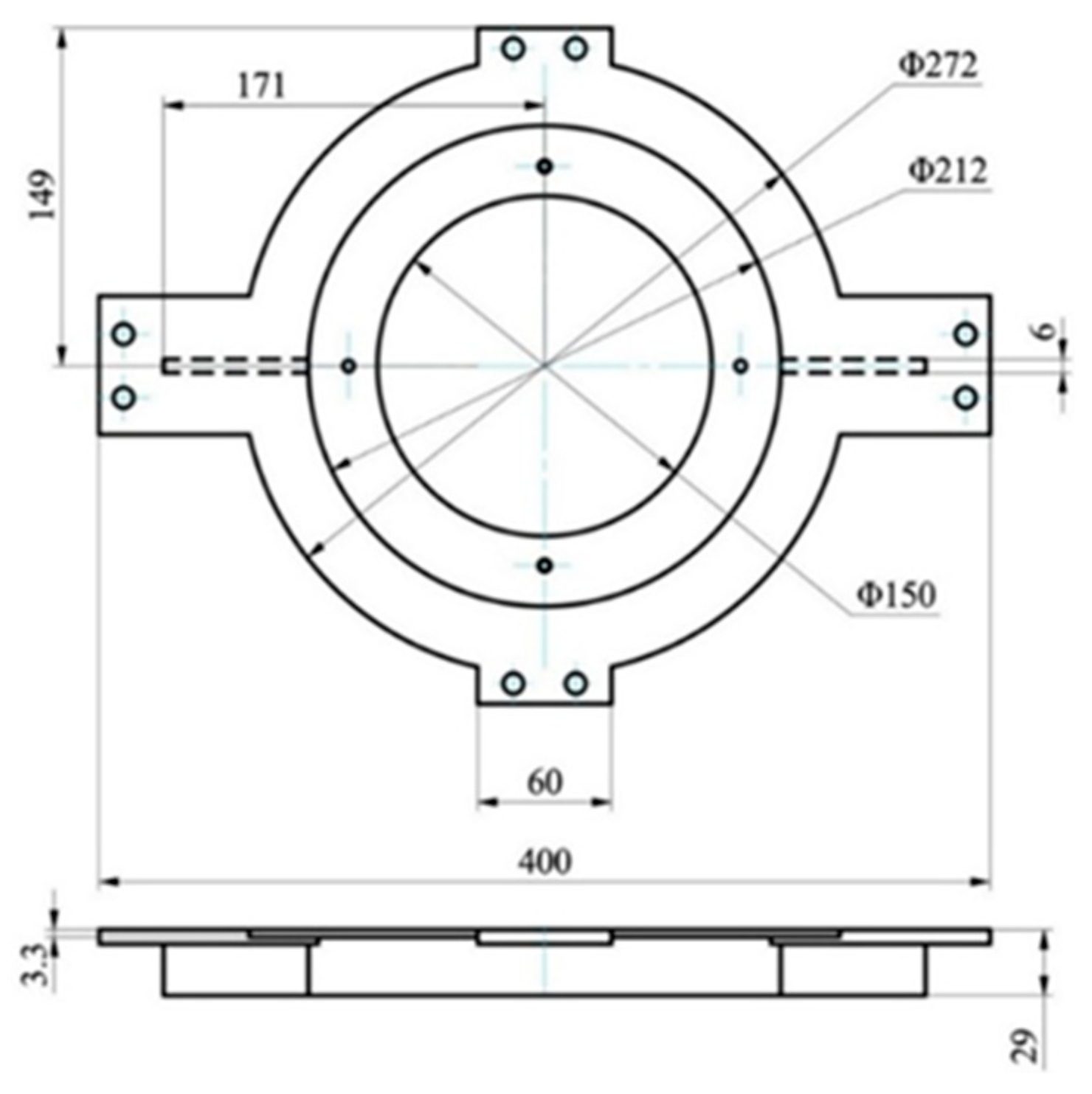
The present case study focuses on a viscoelastic damped bracket designed for the installation of airborne electronic equipment, as shown in Figure 16. This bracket comprises five components: the connecting plate, face plate, side plates, base plate, and reinforcement ribs. The connecting plate is affixed to the external structure using eight M9 bolts, while the base plate is connected to the electronic equipment structure with four M5 bolts. The primary structure of the bracket is fabricated from composite laminates with the following material properties: $E_{11}=140 \mathrm{GPa}$, $E_{22}=E_{33}=10 \mathrm{GPa}$, $G_{12}=G_{13}=G_{23}=5.6 \mathrm{GPa}$, $v_{12}=0.3$, and $\rho =1560 \mathrm{kg}/{\mathrm{m}}^3$. The layering sequence and total laminate thickness for each component are detailed in

Table 6. Layup and thickness for each component of the infrared devices brackets.

Components	Layup (°)	Thickness (mm)
Connecting plate	$[+45/-45/{\left(0/90\right)}_3/-45/+45/\mathrm{core}/+45/-45/{\left(0/90\right)}_3/-45/+45/$ $+45/-45/{\left(0/90\right)}_3/-45/+45/+45/-45/{\left(0/90\right)}_3/-45/+45/]$	6.3
Face plate	$\left[+45/-45/{\left(0/90\right)}_3/-45/+45/\mathrm{core}/+45/-45/{\left(90/0\right)}_3/-45/+45\right]$	3.3
Side plate	${\left[\pm 45/{\left(0/90\right)}_3/\mp 45\right]}_{\mathrm{s}}$	3
Base plate	$\left[+45/-45/{\left(0/90\right)}_3/-45/+45/\mathrm{core}/+45/-45/{\left(90/0\right)}_3/-45/+45\right]$	3.3
Reinforcement ribs	${\left[\pm 45/{\left(0/90\right)}_3/\mp 45\right]}_{\mathrm{s}2}$	6

. The core material, 3M ISD-112, is embedded within the connecting, face, and base plates, measuring 0.3 mm in thickness. Each individual laminate layer has a thickness of 0.15 mm. During the finite element modeling process, the electronic equipment was simulated using concentrated mass elements, with local details such as bolt holes omitted. Fixed support constraints were applied at the external bolt holes, resulting in a layer-wise model with a total of 25,530 DoFs.

Due to the complexity of this actual structure, it is necessary to first conduct a validation for the DRE-MSE method. Subsequently, the first ten modal natural frequencies and damping ratios were computed using the DRE-MSE methods, with an error tolerance set to ${\epsilon }_{\mathrm{t}}=1 \times {10}^{-4}$. The results, presented in

Table 7. The first ten natural frequencies and damping ratios for the viscoelastic damped bracket.

Mode Order	DRE-MSE (29.17 s)		I-IRA (55.22 s)
	Frequency (Hz)	Damping Ratio (%)	Frequency (Hz)	Damping Ratio (%)
1	143.2379	1.7650	143.2385	1.7600
2	146.1872	2.0692	146.1872	2.0693
3	147.8029	2.0177	147.8027	2.0178
4	154.7933	2.0261	154.7933	2.0262
5	529.8576	3.6587	529.8574	3.6576
6	619.5348	4.9441	619.5620	4.9339
7	632.1182	4.3458	632.1183	4.3449
8	808.1331	6.2848	808.1376	6.2827
9	870.0285	3.6407	870.0313	3.6400
10	905.7332	5.3702	905.7384	5.3695

, indicate a strong agreement between the outcomes derived from the I-IRA and DRE-MSE methods. Notably, the former method required 55.22 s, whereas the latter was completed in only 29.17 s.

To enhance the robustness of both stiffness and damping performance, a comprehensive reevaluation of the type and thickness of the core layer material within the connecting plate, face plate, and base plate will be undertaken. The problem does not include deterministic design variables and uncontrollable parameters. The core types in the connecting plate, face plate, and base plate are the same and defined as the uncertain design variable $u_1^0$. Considering four possible viscoelastic materials (#1, #3, #4, and #5), $u_1^0$ is encoded as integers 1, 2, 3, and 4, corresponding to different values of the random variable $U_1$:

• When $u_1^0=1$, the core is made of material #1, with $U_1~\mathrm{N}\left(0.5,{0.025}^2\right)$;
• When $u_1^0=2$, the core is made of material #3, with ${\mathrm{U}}_1~\mathrm{N}\left(0.5542,{0.02771}^2\right)$;
• When $u_1^0=3$, the core is made of material #4, with ${\mathrm{U}}_1~\mathrm{N}\left(1.4,{0.07}^2\right)$;
• When $u_1^0=4$, the core is made of material #5, with ${\mathrm{U}}_1~\mathrm{N}\left(5.0,{0.25}^2\right)$;

The core layer thickness for the connecting plate, face plate, and base plate are also uncertain design variables, defined as $u_2^0,$ $u_3^0$, and $u_4^0$, with real-valued encoding within the range [0.2 mm, 0.5 mm]. For any real value within the feasible domain, the random variables $U_k(k=2,3,4)$ are defined as: $U_2~\mathrm{N}({\mu }_2,{\left(0.05{\mu }_2\right)}^2)$, $U_3~\mathrm{N}({\mu }_3,{\left(0.05{\mu }_3\right)}^2)$, and $U_4~\mathrm{N}({\mu }_4,{\left(0.05{\mu }_4\right)}^2)$, with $\mathbb{E}\left(U_2\right)={\mu }_2=u_2^0$, $\mathbb{E}\left(U_3\right)={\mu }_3=u_3^0$, and $\left(U_4\right)={\mu }_4=u_4^0$.

To maximize the robustness of the objective functions for the first modal natural frequency and damping ratio, the final specific optimization problem is as follows:

$$\left\{\begin{array}{c}\mathrm{f}\mathrm{i}\mathrm{n}\mathrm{d} {\mathit{u}}^0 \\ \mathrm{minimize}\left\{{\varphi }_1\left({\mathit{u}}^0\right),{\varphi }_2\left({\mathit{u}}^0\right)\right\} \\ \mathrm{subject} \mathrm{to} {\mathit{u}}^0={\left[u_1^0,u_2^0,u_3^0,u_4^0\right]}^{\mathrm{T}} \\ u_1^0\in \left\{1,2,3,4\right\} \\ 0.2\le u_k^0\le 0.5 \left(\mathrm{m}\mathrm{m}\right),k=2,3,4\\ u_1^0=1,U_1~\mathrm{N}\left(0.5,{0.025}^2\right) \left(\mathrm{M}\mathrm{P}\mathrm{a}\right)\\ u_1^0=2,U_1~\mathrm{N}\left(0.5542,{0.02771}^2\right) \left(\mathrm{M}\mathrm{P}\mathrm{a}\right)\\ u_1^0=3,U_1~\mathrm{N}\left(1.4,{0.07}^2\right) \left(\mathrm{M}\mathrm{P}\mathrm{a}\right) \\ u_1^0=4,U_1~\mathrm{N}\left(5.0,{0.25}^2\right) \left(\mathrm{M}\mathrm{P}\mathrm{a}\right) \\ U_k~\mathrm{N}\left({\mu }_k,{{\sigma }_k}^2\right),\mathbb{E}\left(U_k\right)={\mu }_k=u_k^0,k=2,3,4\\ {\mathrm{C}\mathrm{o}\mathrm{V}}_k=\left({\sigma }_k/u_k^0\right)\times 100\mathrm{\%}=5\%,k=2,3,4\end{array}\right.$$

(37)

The algorithm parameter settings are as follows: In the DRE-MSE method, the error tolerance is established at 1 × 10⁻⁴. In the NSGA-II algorithm, the population size is set to 100, and the maximum number of evolutionary generations is defined as 50. Figure 17 presents the robust Pareto optimal results for the fundamental frequency and damping characteristics based on the selection of core layer material types and thicknesses of the three plate components. Specifically, the optimization outcomes incorporating various types of viscoelastic damping materials are distinguished by different colors. It is observed that all four types of viscoelastic damping materials appear in the optimal solution, displaying distinct clustering patterns. The red color denotes the optimization results featuring 3M ISD−112 viscoelastic material, which demonstrates excellent stiffness robustness but relatively poor damping robustness. This indicates low dispersion in the fundamental frequency while exhibiting significant dispersion in the fundamental damping characteristics. In contrast, the purple color represents the optimization results utilizing GE SMRD viscoelastic material, which shows outstanding damping robustness but significantly reduced stiffness robustness. Such a configuration is particularly appealing for design products that prioritize the dispersion of fundamental damping characteristics over frequency considerations. Additionally, both blue and cyan colors, representing the results with ZN-1 and DM 9740 viscoelastic damping materials, respectively, exhibit relatively superior robustness in both stiffness and damping, reflecting a more balanced design intent.

Subsequently, we identified the design solutions exhibiting either the best stiffness robustness or the best damping robustness from the results presented in Figure 17, which utilized different viscoelastic damping materials. These solutions are denoted by the labels A, B, C, D, E, F, G, and H, with the specific design variable parameters provided in

Table 8. Robust design results for schemes A–H.

Scheme	Design Variables				RDO
	$\mathbf{Core} \mathbf{Type}, {\mathit{u}}_1$	${\mathit{u}}_2$ (mm)	${\mathit{u}}_2$ (mm)	${\mathit{u}}_2$ (mm)	${\mathit{\varphi }}_1$	${\mathit{\varphi }}_2$
A	1	0.5000	0.3224	0.5000	0.0841	0.7097
B	1	0.2000	0.2000	0.2000	0.1239	0.5612
C	2	0.5000	0.3313	0.5000	0.1243	0.4222
D	2	0.2000	0.2000	0.2000	0.1806	0.3960
E	3	0.5000	0.2000	0.5000	0.5216	0.3380
F	3	0.2175	0.3565	0.2301	0.6778	0.2279
G	4	0.2145	0.5000	0.5000	0.6791	0.1478
H	4	0.2194	0.4513	0.3880	0.6957	0.1202

.

6. Conclusions

In summary, this study presents a novel approach for robust design optimization (RDO) of viscoelastic damped composite structures aiming to enhance the robustness of dynamic characteristics, which are susceptible to variabilities in material properties and geometrical configurations. Specifically, we introduce a projection-based model order reduction (MOR) method tailored for single-sample analysis challenged by nonlinear eigenvalue problems. For uncertainty propagation (UP) analysis, we develop a generalized stochastic collocation (gSC) method that employs statistical moment computation techniques, accommodating arbitrary random distributions. The synergistic combination of advanced model reduction techniques, UP methodologies, and intelligent multi-objective optimization algorithms enhances computational efficiency while ensuring necessary accuracy.

The results from four examples demonstrate the efficacy of the proposed MOR and gSC methods, as well as the overall RDO framework. Importantly, the RDO results provide a comprehensive analysis of the impact of considering uncertainty factors in design processes. They demonstrate that the RDO approach effectively reduces the sensitivity of structural performance to various uncertainties, thereby enhancing the reliability and robustness of the designs. These findings illuminate the critical importance of integrating uncertainty considerations into the design optimization process.

References

1. Rajak, D.K.; Pagar, D.D.; Menezes, P.L.; Linul, E. Fiber-Reinforced Polymer Composites: Manufacturing, Properties, and Applications. Polymers 2019, 11, 1667. [Google Scholar] [CrossRef] [PubMed]
2. Chandra, R.; Singh, S.P.; Gupta, K. Damping Studies in Fiber-Reinforced Composites—A Review. Compos. Struct. 1999, 46, 41–51. [Google Scholar] [CrossRef]
3. Nakra, B.C. Vibration Control in Machines and Structures Using Viscoelastic Damping. J. Sound Vib. 1998, 211, 449–466. [Google Scholar] [CrossRef]
4. Zhou, X.Q.; Yu, D.Y.; Shao, X.Y.; Zhang, S.Q.; Wang, S. Research and Applications of Viscoelastic Vibration Damping Materials: A Review. Compos. Struct. 2016, 136, 460–480. [Google Scholar] [CrossRef]
5. Abrate, S.; Di Sciuva, M. Equivalent Single Layer Theories for Composite and Sandwich Structures: A Review. Compos. Struct. 2017, 179, 482–494. [Google Scholar] [CrossRef]
6. Birman, V.; Kardomateas, G.A. Review of Current Trends in Research and Applications of Sandwich Structures. Compos. Part B-Eng. 2018, 142, 221–240. [Google Scholar] [CrossRef]
7. Khandan, R.; Noroozi, S.; Sewell, P.; Vinney, J. The Development of Laminated Composite Plate Theories: A Review. J. Mater. Sci. 2012, 47, 5901–5910. [Google Scholar] [CrossRef]
8. Liew, K.M.; Pan, Z.Z.; Zhang, L.W. An Overview of Layerwise Theories for Composite Laminates and Structures: Development, Numerical Implementation and Application. Compos. Struct. 2019, 215, 240–259. [Google Scholar] [CrossRef]
9. Lin, R.M.; Lim, M.K. Complex Eigensensitivity-Based Characterization of Structures with Viscoelastic Damping. J. Acoust. Soc. Am. 1996, 100, 3182–3191. [Google Scholar] [CrossRef]
10. Vasques, C.M.A.; Moreira, R.A.S.; Rodrigues Dias, J. Viscoelastic Damping Technologies—Part I: Modeling and Finite Element Implementation. J. Adv. Res. Mech. Eng. 2010, 1, 76–95. [Google Scholar]
11. Adhikari, S.; Pascual, B. Eigenvalues of Linear Viscoelastic Systems. J. Sound Vib. 2009, 325, 1000–1011. [Google Scholar] [CrossRef]
12. Singh, K.V. Eigenvalue and Eigenvector Computation for Discrete and Continuous Structures Composed of Viscoelastic Materials. Int. J. Mech. Sci. 2016, 110, 127–137. [Google Scholar] [CrossRef]
13. Daya, E.M.I.; Potier-Ferry, M. A Numerical Method for Nonlinear Eigenvalue Problems Application to Vibrations of Viscoelastic Structures. Comput. Struct. 2001, 79, 533–541. [Google Scholar] [CrossRef]
14. Mallil, E.; Lahmam, H.; Damil, N.; Potier-Ferry, M. An Iterative Process Based on Homotopy and Perturbation Techniques. Comput. Methods Appl. Mech. Eng. 2000, 190, 1845–1858. [Google Scholar] [CrossRef]
15. Mehrmann, V.; Schroder, C. Nonlinear Eigenvalue and Frequency Response Problems in Industrial Practice. J. Math. Ind. 2011, 1, 7. [Google Scholar] [CrossRef]
16. Yokota, S.; Sakurai, T. A Projection Method for Nonlinear Eigenvalue Problems Using Contour Integrals. JSIAM Lett. 2013, 5, 41–44. [Google Scholar] [CrossRef]
17. Voss, H. An Arnoldi Method for Nonlinear Eigenvalue Problems. Bit Numer. Math. 2004, 44, 387–401. [Google Scholar] [CrossRef]
18. Voss, H. A Jacobi-Davidson Method for Nonlinear and Nonsymmetric Eigenproblems. Comput. Struct. 2007, 85, 1284–1292. [Google Scholar] [CrossRef]
19. Hamdaoui, M.; Akoussan, K.; Daya, E.M.I. Comparison of Non-Linear Eigensolvers for Modal Analysis of Frequency Dependent Laminated Viscoelastic Sandwich Plates. Finite Elem. Anal. Des. 2016, 121, 75–85. [Google Scholar] [CrossRef]
20. Johnson, C.D.; Kienholz, D.A. Finite Element Prediction of Damping in Structures with Constrained Viscoelastic Layers. AIAA J. 1982, 20, 1284–1290. [Google Scholar] [CrossRef]
21. Rikards, R.; Chate, A.; Barkanov, E. Finite Element Analysis of Damping the Vibrations of Laminated Composites. Comput. Struct. 1993, 47, 1005–1015. [Google Scholar] [CrossRef]
22. Hu, B.; Dokainish, M.A.; Mansour, W.M. A Modified MSE Method for Viscoelastic Systems: A Weighted Stiffness Matrix Approach. J. Vibration Acoust. 1995, 117, 226–231. [Google Scholar] [CrossRef]
23. Trindade, M.A.; Benjeddou, A.; Ohayon, R. Modeling of Frequency-Dependent Viscoelastic Materials for Active-Passive Vibration Damping. J. Vibration Acoust. 2000, 122, 169–174. [Google Scholar] [CrossRef]
24. D’Ottavio, M.; Krasnobrizha, A.; Valot, E.; Polit, O.; Vescovini, R.; Dozio, L. Dynamic Response of Viscoelastic Multiple-Core Sandwich Structures. J. Sound Vib. 2021, 491, 115753. [Google Scholar] [CrossRef]
25. Bilasse, M.; Daya, E.M.I.; Azrar, L. Linear and Nonlinear Vibrations Analysis of Viscoelastic Sandwich Beams. J. Sound Vib. 2010, 329, 4950–4969. [Google Scholar] [CrossRef]
26. Boumediene, F.; Cadou, J.M.; Duigou, L.; Daya, E.M.I. A Reduction Model for Eigensolutions of Damped Viscoelastic Sandwich Structures. Mech. Res. Commun. 2014, 57, 74–81. [Google Scholar] [CrossRef]
27. Rouleau, L.; Deü, J.F.; Legay, A. A Comparison of Model Reduction Techniques Based on Modal Projection for Structures with Frequency-Dependent Damping. Mech. Syst. Signal Process. 2017, 90, 110–125. [Google Scholar] [CrossRef]
28. Araujo, A.L.; Soares, C.M.M.; Soares, C.A.M.; Herskovits, J. Optimal Design and Parameter Estimation of Frequency Dependent Viscoelastic Laminated Sandwich Composite Plates. Compos. Struct. 2010, 92, 2321–2327. [Google Scholar] [CrossRef]
29. Le Maoût, N.; Verron, E.; Bègue, J. Simultaneous Geometrical and Material Optimal Design of Hybrid Elastomer/Composite Sandwich Plates. Compos. Struct. 2011, 93, 1153–1157. [Google Scholar] [CrossRef]
30. Montemurro, M.; Koutsawa, Y.; Belouettar, S.; Vincenti, A.; Vannucci, P. Design of Damping Properties of Hybrid Laminates Through a Global Optimization Strategy. Compos. Struct. 2012, 94, 3309–3320. [Google Scholar] [CrossRef]
31. Hamdaoui, M.; Robin, G.; Jrad, M.; Daya, E.M.I. Optimal Design of Frequency Dependent Three-Layered Rectangular Composite Beams for Low Mass and High Damping. Compos. Struct. 2015, 120, 174–182. [Google Scholar] [CrossRef]
32. Madeira, J.F.A.; Araújo, A.L.; Soares, C.M.M.; Soares, C.A.M. Multiobjective Optimization of Viscoelastic Laminated Sandwich Structures Using the Direct MultiSearch Method. Comput. Struct. 2015, 147, 229–235. [Google Scholar] [CrossRef]
33. Arikoglu, A. Multi-Objective Optimal Design of Hybrid Viscoelastic/Composite Sandwich Beams by Using the Generalized Differential Quadrature Method and the Non-Dominated Sorting Genetic Algorithm II. Struct. Multidiscip. Optim. 2017, 56, 885–901. [Google Scholar] [CrossRef]
34. Pathan, M.V.; Patsias, S.; Tagarielli, V.L. A Real-Coded Genetic Algorithm for Optimizing the Damping Response of Composite Laminates. Comput. Struct. 2018, 198, 51–60. [Google Scholar] [CrossRef]
35. Valvano, S.; Orlando, C.; Alaimo, A. Design of a Noise Reduction Passive Control System Based on Viscoelastic Multilayered Plate Using PDSO. Mech. Syst. Signal Process. 2019, 123, 153–173. [Google Scholar] [CrossRef]
36. Li, J.; Narita, Y. Analysis and Optimal Design for the Damping Property of Laminated Viscoelastic Plates Under General Edge Conditions. Compos. Part B Eng. 2013, 45, 972–980. [Google Scholar] [CrossRef]
37. Akoussan, K.; Hamdaoui, M. Improved Layer-Wise Optimization Algorithm for the Design of Viscoelastic Composite Structures. Compos. Struct. 2017, 176, 342–358. [Google Scholar] [CrossRef]
38. Beyer, H.G.; Sendhoff, B. Robust Optimization—A Comprehensive Survey. Comput. Methods Appl. Mech. Eng. 2007, 196, 3190–3218. [Google Scholar] [CrossRef]
39. Guedri, M.; Lima, A.M.G.; Bouhaddi, N.; Rade, D.A. Robust Design of Viscoelastic Structures Based on Stochastic Finite Element Models. Mech. Syst. Signal Process. 2010, 24, 59–77. [Google Scholar] [CrossRef]
40. Jaboviste, K.; Sadoulet-Reboul, E.; Peyret, N.; Arnould, C.; Collard, E.; Chevallier, G. On the Compromise Between Performance and Robustness for Viscoelastic Damped Structures. Mech. Syst. Signal Process. 2019, 119, 65–80. [Google Scholar] [CrossRef]
41. Hernández, W.P.; Castello, D.A.; Ritto, T.G. Uncertainty Propagation Analysis in Laminated Structures with Viscoelastic Core. Comput. Struct. 2016, 164, 23–37. [Google Scholar] [CrossRef]
42. Druesne, F.; Hamdaoui, M.; Lardeur, P. Variability of Dynamic Responses of Frequency Dependent Viscoelastic Sandwich Beams with Material and Physical Properties Modeled by Spatial Random Fields. Compos. Struct. 2016, 152, 316–323. [Google Scholar] [CrossRef]
43. Silva, V.A.C.; Lima, A.M.G.; Bouhaddi, N.; Lacerda, H.B. Uncertainty Propagation and Experimental Verification of Nonlinear Viscoelastic Sandwich Beams. Mech. Syst. Signal Process. 2019, 132, 654–669. [Google Scholar] [CrossRef]
44. Xiu, D.B.; Hesthaven, J.S. High-Order Collocation Methods for Differential Equations with Random Inputs. SIAM J. Sci. Comput. 2005, 27, 1118–1139. [Google Scholar] [CrossRef]
45. Wang, T.Y.; Xu, C.; Hamdaoui, M.; Guo, N.; Gu, L.X. Uncertainty Propagation in Modal Analysis of Viscoelastic Sandwich Structure Using a Stochastic Collocation Method. J. Sandwich Struct. Mater. 2021, 23, 1141–1165. [Google Scholar] [CrossRef]
46. Wang, T.Y.; Xu, C.; Guo, N.; Hamdaoui, M.; Daya, E.M.I. Uncertainty Propagation of Frequency Response of Viscoelastic Damping Structures Using a Modified High-Dimensional Adaptive Sparse Grid Collocation Method. Mech. Adv. Mater. Struct. 2020, 29, 506–524. [Google Scholar] [CrossRef]
47. Wang, T.Y.; Xu, C.; Guo, N. A Novel Frequency-Labeled Adaptive Sparse Grid Collocation Method for Uncertainty Quantification of the Frequency Response of General Viscoelastic Damping Structures. Int. J. Mech. Sci. 2021, 193, 106168. [Google Scholar] [CrossRef]
48. Bagley, R.L.; Torvik, P.J. Fractional Calculus—A Different Approach to the Analysis of Viscoelastically Damped Structures. AIAA J. 1983, 21, 741–748. [Google Scholar] [CrossRef]
49. Golla, D.F.; Hughes, P.C. Dynamics of Viscoelastic Structures—A Time-Domain, Finite Element Formulation. J. Appl. Mech. 1985, 52, 897–906. [Google Scholar] [CrossRef]
50. Lesieutre, G.A.; Mingori, D.L. Finite Element Modeling of Frequency-Dependent Material Damping Using Augmenting Thermodynamic Fields. J. Guid. Control Dyn. 1990, 13, 1040–1050. [Google Scholar] [CrossRef]
51. Xu, C.; Wu, M.Z.; Hamdaoui, M. Mixed Integer Multi-Objective Optimization of Composite Structures with Frequency-Dependent Interleaved Viscoelastic Damping Layers. Comput. Struct. 2016, 172, 81–92. [Google Scholar] [CrossRef]
52. Xu, C.; Lin, S.; Yang, Y.Z. Optimal Design of Viscoelastic Damping Structures Using Layerwise Finite Element Analysis and Multi-Objective Genetic Algorithm. Comput. Struct. 2015, 157, 1–8. [Google Scholar] [CrossRef]
53. Gautschi, W. Orthogonal Polynomials: Computation and Approximation; Oxford University Press: Oxford, UK, 2004. [Google Scholar]
54. Golub, G.H.; Welsch, J.H. Calculation of Gauss Quadrature Rules. Math. Comput. 1969, 23, 221. [Google Scholar] [CrossRef]
55. Smolyak, S.A. Quadrature and Interpolation Formulas for Tensor Products of Certain Classes of Functions. Dokl. Akad. Nauk 1963, 148, 1042–1045. [Google Scholar]
56. Wan, H.P.; Ren, W.X.; Todd, M.D. Arbitrary Polynomial Chaos Expansion Method for Uncertainty Quantification and Global Sensitivity Analysis in Structural Dynamics. Mech. Syst. Signal Process. 2020, 142, 106732. [Google Scholar] [CrossRef]
57. Mysovskih, I.P. On the Construction of Cubature Formulas with the Smallest Number of Nodes. Dokl. Akad. Nauk 1968, 178, 1252–1254. [Google Scholar]
58. Sasikumar, P.; Suresh, R.; Gupta, S. Stochastic Model Order Reduction in Uncertainty Quantification of Composite Structures. Compos. Struct. 2015, 128, 21–34. [Google Scholar] [CrossRef]
Figure 1. Frequency−dependent characteristics of six viscoelastic materials over the range from 1 Hz to 1000 Hz. (a) Storage modulus; (b) Loss factor.
Aerospace 11 01038 g001
Figure 2. The kinematic model of the n-layer viscoelastic damped composite structure.
Aerospace 11 01038 g002
Figure 3. Four types of design variables diagram. (a) Two design variables of thickness and material of viscoelastic damping layer; (b) Two design variables of embedded position of viscoelastic damping layer and angle of composite ply.
Aerospace 11 01038 g003
Figure 4. Composition of 50 chromosomes in an RDO: deterministic design variables, uncertain design variables, and uncontrollable parameters.
Aerospace 11 01038 g004
Figure 5. Robust multi-objective optimization design framework for viscoelastic damped composite structures.
Aerospace 11 01038 g005
Figure 6. A four−sided simply supported sandwich viscoelastic damped panel. (a) Geometric diagram; (b) First four undamped modes.
Aerospace 11 01038 g006
Figure 7. Computational costs of four methods for six different frequency-dependent viscoelastic sandwich core structures.
Aerospace 11 01038 g007
Figure 8. Relationship between average relative errors and computation costs using DRE-MSE and I-IRA methods under different convergence tolerance requirements for structures with 9570 DoFs.
Aerospace 11 01038 g008
Figure 9. Relationship between average relative errors and computation costs using DRE-MSE and I-IRA methods under different convergence tolerance requirements for structures with 37,050 DoFs.
Aerospace 11 01038 g009
Figure 10. Geometry and layout of a four-sided fixed viscoelastic damped laminated plate.
Aerospace 11 01038 g010
Figure 11. Comparison of the convergence of the MCS and gSC methods. (a) Expectations for natural frequencies; (b) Standard deviations for natural frequencies; (c) Expectations for damping ratios; (d) Standard deviations for natural frequencies.
Aerospace 11 01038 g011
Figure 12. PDFs results obtained using both the MCS and gSC methods. (a) PDF of the first natural frequency; (b) PDF of the second natural frequency; (c) PDF of the third natural frequency; (d) PDF of the fourth natural frequency; (e) PDF of the first damping ratio; (f) PDF of the second damping ratio; (g) PDF of the third damping ratio; (h) PDF of the fourth damping ratio.
Aerospace 11 01038 g012
Figure 13. Schematic diagram of the beam plate.
Aerospace 11 01038 g013
Figure 14. Pareto optimal solutions for deterministic and three uncertain scenarios. (a) Deterministic optimization case; (b) RDO case 1; (c) RDO case 2; (d) RDO case 3.
Aerospace 11 01038 g014
Figure 15. Comparison of optimal designs under four scenarios. (a) Design spaces for the four scenarios; (b) Optimal design points in the nominal objectives of the deterministic case; (c) Optimal design points in the robust objectives of RDO Case 3.
Aerospace 11 01038 g015
Figure 16. Diagram of the dimensions of the infrared devices brackets.
Aerospace 11 01038 g016
Figure 17. Robust Pareto optimal results for fundamental frequency and damping characteristics.
Aerospace 11 01038 g017