Abstract
Complex microscopic simulation models of strategic Air Traffic Management (ATM) performance assessment and decision-making are hindered by several factors. One of the most important is the existence of hidden parameters—such as aircraft take-off weight (TOW) and the selected cost index (CI)—which, if known, would allow for more effective performance modeling methodologies for assessing Key Performance Indicators (KPIs) at various levels of abstraction/detail, e.g., system-wide, or at the level of individual flights. This research proposes a data-driven methodology for the estimation of flights’ hidden parameters combining mechanistic and advanced Artificial Intelligence/Machine Learning (AI/ML) models. Aiming at microsimulation models, our goal is to study the effect of these estimations on the prediction of flights’ KPIs. In so doing, we propose a novel methodology according to which data-driven methods are trained given optimal trajectories (produced by mechanistic models) corresponding to known hidden parameter values, with the aim of predicting hidden parameters’ values of unseen trajectories. The results show that estimations of hidden parameters support the accurate prediction of KPIs regarding the efficiency of flights: fuel consumption, gate-to-gate time and distance flown.
Keywords:
prediction; hidden parameters; KPIs; take-off weight; cost index; deep learning; simulation 1. Introduction
Air Traffic Management (ATM) aims at maintaining a safe and efficient flow of traffic. However, it typically entails a set of constraints that may affect the environment by the increment of CO2 emissions. In this context, ATM modernization initiatives such as SESAR in Europe and NextGen in the U.S. introduce new concepts and solutions intended to reduce environmental inefficiencies. Consequently, the performance of such concepts/solutions should be regularly evaluated against environmental goals and other ATM objectives. This performance assessment helps to identify gaps between current outcomes and high-level targets, thereby guiding necessary corrective actions to bridge these gaps.
In this regard, the International Civil Aviation Organization (ICAO) initiated a global effort in 2003 to create a performance-based approach for the future of the global ATM system [,], which was supported by the Civil Air Navigation Services Organization (CANSO) []. Reflecting these global efforts, Europe has adopted the Single European Sky (SES) Performance Scheme, a structured approach to set, measure, baseline, and benchmark ATM performance targets []. An extensive review comparing performance frameworks developed by ICAO, CANSO, the SES Performance Scheme, and the SESAR 2020 performance framework is provided in []. This review identifies over 150 Key Performance Indicators (KPIs) used for managing and monitoring performance across 11 distinct key performance areas (KPAs). Similarly, the NextGen program in the U.S. has also developed numerous KPIs to monitor the effectiveness of its deployment efforts [,].
Hence, the development of performance modeling methodologies, able to grasp the interdependencies between different KPAs and translate ATM concepts and technologies into their impact on KPIs, has been a long-time objective of the ATM research community. Generally speaking, the modeling approaches to this problem can be classified into two main categories: macroscopic and microscopic. Macroscopic models (e.g., []) represent the behavior of a system by formulating the relationships between aggregated variables without explicitly modeling the individual system components. On the contrary, microscopic models (e.g., [,]) adopt an explicit representation of the actions and interactions of the individual elements that compose a system with the aim to observe the performance that emerges at the macroscopic level. Several SESAR exploratory research projects, such as APACHE (www.sesarju.eu/projects/apache, accessed on 12 September 2024), Vista (https://www.sesarju.eu/projects/vista, accessed on 12 September 2024) and EvoATM (www.sesarju.eu/projects/evoATM, accessed on 12 September 2024), have employed different types of microscopic models (e.g., agent-based models) to understand the influence of new ATM concepts and solutions on the performance of the system as a whole, showing the ability of these models to capture a rich variety of behaviors in a very realistic manner. However, the practical application of complex simulation models to strategic ATM performance assessment and decision-making is hindered by several factors. One of the most important is that these microscopic models often need parameters that are hidden: even if they could, in principle, be measured, certain aspects of the ATM system may not be observable for practical reasons. This is the case, for example, for business-sensitive data related to the behavior of airspace users (AUs) that are of paramount importance for the construction of microsimulation models, such as aircraft take-off weight (TOW) and the selected cost index (CI (The cost index, which is of importance here, is a parameter chosen by the airspace user and reflects the relative importance of the cost of time with respect to fuel costs []. High values of CI mean that the cost of time is significantly more important than the cost of fuel. This is translated into higher speeds and different lateral/vertical profiles)), among others. See for instance the fuel and distance efficiency metrics proposed in [], which represent an advance in the state of the art in measuring ATM performance, but which required a knowledge or estimation of these hidden parameters.
In the last decade, with the rising interest in artificial intelligence, transport and traffic modelers have begun to apply a variety of machine-learning techniques for hidden parameter estimation that are proving successful in improving the capabilities of microsimulation models [,,]. However, the exploration of these techniques in the field of ATM is only very recent. A common approach in many simulation exercises is to set these unknown or non-observable parameters based on some typical values recommended in the literature, due to the difficulties to conduct a rigorous and systematic calibration on them []. However, these parameters can differ significantly across AUs. The question, as in any calibration exercise, is essentially how to explore the parameter space of each AU model in order to find the combination of parameter values that better matches the observed trajectory choices of that AU. The problem is therefore similar to that of efficiently exploring the model input–output space. This problem has been addressed in SIMBAD []. In this paper, we propose a data-driven methodology for the estimation of flights’ hidden parameters combining mechanistic and advanced Artificial Intelligence/Machine Learning (AI/ML) models, studying also the effect of these estimations on the prediction of flights’ KPIs.
The problem of estimating flights’ hidden parameters has been addressed in [], who aimed to estimate take-off weight (TOW) and speed profile during climb, using a stochastic gradient boosting tree algorithm. This aims at a prediction (before take-off) approach without considering flight plans, i.e., AUs’ preferences and intentions. Instead of TOW, researchers in [] aimed at estimating aircraft mass using example trajectories. However, since the actual values of the hidden parameters were not known, they fit their model to estimate the adjusted mass in terms of the observed energy rate of future trajectory points. A similar approach is considered in [], where machine-learning methods are used, in a manner that is close to what we do here and what we have done in []. Also targeting the estimation of aircraft mass, the authors in [] used Quick Access Recorder (QAR) data, taking advantage of a combination of model-based and data-driven approaches. Specifically, they used a multi-layer perceptron neural network (MLPNN) to approximate the model-based estimation function. Other proposals for estimating TOW include statistical approaches in [], using Gaussian Process Regression (GPR) and data from aircraft take-off ground roll. Similarly to our study, they also considered the prediction of fuel flow rates. Also, Sun et al. [,,,] proposed statistical methods to estimate aircraft mass, given that Artificial Intelligence/Machine Learning (AI/ML) need ground truth values, which in general are not known.
Given that the main objective of this research is to explore the use of AI/ML techniques for the estimation of flights’ hidden parameters, with the aim of predicting flights’ KPIs, in contrast to previous approaches, we propose training AI/ML methods using example trajectories produced by mechanistic models, with known values of the target hidden parameters. Specifically, we exploit flight plans, revealing AUs’ intentions, and data from all the flight phases. In so doing, we do not use “proxies” to measure the accuracy of models (e.g., fuel consumption, energy rate or the trajectory itself). This allows us to use the hidden variables’ estimations for different purposes. Here, we study the effect of hidden variables’ estimations on the prediction of the following KPIs: (a) fuel consumption, (b) distance flown, (c) and gate-to-gate time.
More specifically, this paper presents a novel data-driven methodology for the estimation of payload (The payload refers to all the mass that is taken by an airplane, excluding fuel. The amount of payload and the amount of fuel that is embarked to fly over a specific distance are limited by the aircraft maximum take-off weight (see also in http://www.aerostudents.com/courses/aerospace-design-and-systems-engineering-elements-1/PayloadRangeDiagrams.pdf, accessed on 12 September 2024)) mass (PL) and cost index (CI) parameters, combining mechanistic and AI/ML models. Both the CI and PL are crucial in terms of KPIs’ estimation and in particular to fuel estimation.
According to the proposed methodology, mechanistic models produce optimal trajectories with respect to specific hidden parameters values, and data-driven methods are trained to predict the hidden parameters’ values, given these flight trajectories. In a previous article [], we have evaluated several AI/ML methods to estimate PL and CI, examining how these estimations affect the prediction of KPIs regarding the efficiency of flights. This paper goes beyond the work reported in [] by proposing a novel deep-learning method for the estimation of the PL and CI, in comparison to the best method reported in []. The results show the effects of hidden variables’ predictions on the accurate prediction of flights’ KPIs, which is of outmost importance to modeling and inferring the performance of flights in relation to ATM concepts.
The contributions that this paper makes are summarized as follows:
- First, it contributes a specific methodology for the data-driven estimation of hidden parameters, using mechanistic models for the provision of training examples.
- Second, AI/ML and deep-learning methods are devised, tuned and evaluated for the estimation of hidden parameters. Specifically, a novel deep-learning method based on graph convolution networks is proposed and evaluated for the estimation of hidden parameters, also in comparison to the best ML method studied in [].
- Third, data-driven AI/ML models are evaluated in the context of the overall methodology where specific flights’ KPIs are predicted, providing a set of comprehensive, comparative results: This shows how the hidden parameters’ estimations of advanced AI/ML methods affect the accurate prediction of specific KPIs.
The structure of this paper is as follows: Section 2 includes (a) the presentation of the overall methodology towards training AI/ML models for the estimation of hidden parameters and the prediction of KPIs, (b) describes the datasets exploited for training/testing the AI/ML models, and (c) presents the problem formulation and the AI/ML methods used for the estimation of hidden parameters. Section 3 presents results from these methods for the estimation of flights’ hidden parameters. Section 4 discusses findings and shows how hidden parameters estimated by the AI/ML methods affect the prediction of flights’ KPIs. Section 5 concludes the paper with final remarks and future work.
2. Materials and Methods
2.1. Methodology
Figure 1 specifies the overall methodology for the estimation of hidden parameters and prediction of flights’ KPIs. It specifies the pipelines with components for the provision of training/testing data, AI/ML methods, as well as components for the prediction of KPIs.
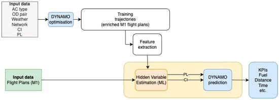
Figure 1.
Overall data-driven methodology for the estimation of hidden variables and prediction of KPIs.
Specifically, Figure 1 shows two pipelines: One for the training of AI/ML models (top) and one (bottom) for using the models for estimating hidden parameters, which concludes with the prediction of KPIs. These pipelines comprise the usage of DYNAMO in optimization and prediction modes.
DYNAMO [] is an aircraft trajectory prediction and optimization engine capable of computing trajectories using realistic and accurate weather, and aircraft performance data with efficiency. DYNAMO is based on an aircraft point-mass model (3 DoF), and its design enables it to be used on real-time applications and/or when a large set of trajectories needs to be generated for simulation, benchmarking purposes, or for training AI/ML methods, as we do here. DYNAMO is highly flexible and configurable and allows the user to specify a great variety of constraints and objective functions.
In the context of the proposed methodology, DYNAMO is used to (a) create training/testing datasets to train/evaluate the AI/ML models, as shown in the first (upper) pipeline in Figure 1; and (b) to predict flights’ KPIs in a mechanistic way, as shown in the second (lower) pipeline of that figure.
Operating in optimization mode, DYNAMOoptimization provides trajectories (flight plans) whose points are enriched with several variables (specified subsequently), along with known values of the hidden parameters’ cost index (CI) and payload mass (PL) for each trajectory. These trajectories and parameters’ target values are used for training the AI/ML models. Flight plans provided by DYNAMOoptimization are called DYNAMO_FP trajectories. The input variables for DYNAMOoptimization are as follows:
- Weather data: Gridded binary (GRIB) meteorological file with wind, pressure and temperature at different geographical locations and altitudes;
- Cost Index (CI);
- Payload mass (PL);
- Aircraft type;
- Origin–destination (OD) pair;
- Airspace structure (free route areas, entry/exit points, airways in non-free route areas, etc.);
- Route charges (if flying in Europe).
DYNAMO optimizes the trajectory following a conventional speed profile, where the typical 250 kt speed limitation below FL100 is observed; climbs and descents are flown at economic (ECON) speeds following a typical Calibrated Airspeed (CAS)–Mach number profile []; and cruise is flown at the cruise ECON Mach. These ECON speeds (CAS or Mach) are influenced by several factors, including the aircraft’s mass, the longitudinal wind, the altitude and the CI. Similar to state-of-the-art flight management systems, DYNAMO obtains these speeds from pre-optimized look-up tables considering such variables, as indicated in detail in []. Then, the optimal altitude profile (including the location of the top of climb and top of descent, along with eventual step climbs during cruise) is obtained by a simple tree-exploration using some heuristics. This approach significantly accelerates the trajectory optimization process.
The second pipeline takes as input a trajectory (flight plan) and uses the trained AI/ML model to estimate the hidden parameters’ values. This time, DYNAMO operates in prediction mode (denoted by DYNAMOprediction) to estimate for the given trajectory the target flight KPIs, given the estimated hidden parameters.
It must be noted that the role of DYNAMOoptimization is to produce datasets of trajectories that are optimal for different combinations of hidden parameter values. These trajectories serve as typical examples to train AI/ML models to estimate hidden parameters for any trajectory. Therefore, after the training of models, DYNAMOoptimization is not necessary for the estimation of hidden parameters and the prediction of KPIs. Also, DYNAMOprediction can be replaced by any other mechanistic model that, given trajectories and the corresponding values of hidden parameters, can predict flights’ KPIs. However, the incorporation of different optimization and prediction models is part of future work. For the purposes of this work, DYNAMOoptimization and DYNAMOprediction are independent modules and do not share any kind of information.
2.2. Datasets
The datasets exploited from these pipelines are as follows:
- Weather conditions data;
- Flight plans;
- Simulated flight data (DYNAMO_FP).
The first dataset provides weather conditions on a predefined spatial grid of fixed positions and time intervals. The data have been retrieved from the Copernicus Climate Change Service (C3S) at ECMWF, covering 28 days in the period of January 2018 to December 2018. This data source provides hourly estimates of many atmospheric, land and oceanic climate variables. The data cover the Earth on a 30 km grid and resolve the atmosphere using 137 levels from the surface up to a height of 80 km.
For the second dataset, EUROCONTROL provides for operational stakeholders an accurate picture of past and future air traffic demand over the European continent via the Demand Data Repository (DDR2). The flight plans in this dataset are provided in the ALLFT+ format (ver. 4). Each record in an ALLFT+ file reports the flight plan of a single flight in 181 columns. Each flight plan comprises at most three profiles: (a) Filed Tactical Flight Model (FTFM or M1); (b) Regulated Tactical Flight Model (RTFM or M2); and (c) Current Tactical Flight Model (CTFM or M3).
For the purposes of this study, we use only M1 flight plans for a specific origin–destination pair: Charles de Gaulle (LFPG) to Istanbul Ataturk airports (LTBA). These are depicted in Figure 2. The choice of M1 plans is not a restriction, since other types of trajectories could be chosen, but we consider that M1 plans better pronounce the preferences of AUs.
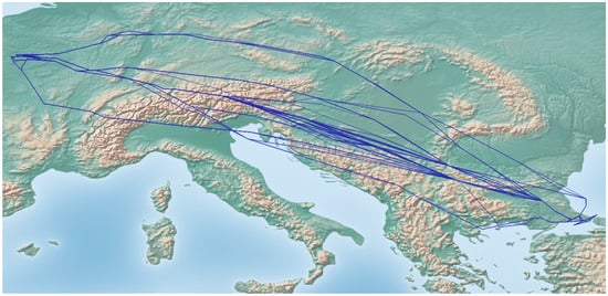
Figure 2.
M1 trajectories in the flight plans’ dataset shown in blue.
Finally, the third dataset includes DYNAMO_FP. The DYNAMO_FP dataset reports 201 distinct flights, which connect Charles de Gaulle (LFPG) and Istanbul Ataturk airports (LTBA), corresponding to the ALLFT+ M1 flight plans shown in Figure 2, operated during any of the 28 days for which weather conditions are available.
Specifically, DYNAMO_FP includes DYNAMOoptimization simulated trajectories, corresponding to the 201 ALLFT+ M1 flight plans, for the 250 possible combinations of 50 CI (ranging from 0 to 100 kg/min, with a discretization interval of 2 kg/min) and 5 PL distinct values, expressed as a fraction of the maximum payload mass (ranging from 0 to 1, with a discretization interval of 0.2). This dataset comprises 50.250 files, i.e., one file for each simulated trajectory for a given combination of CI and PL values.
As provided by DYNAMO, each record reports the position of the aircraft for a specific time (UTC), its altitude (both geometric and pressure altitudes), vertical and horizontal speed and throttle, the computed phase of the trajectory, as well as weather conditions for the given altitude, position and time.
Since some of the variables enriching DYNAMO_FP trajectories are not provided for actual flight plans or can be approximated given flight plans, an additional dataset of pre-processed trajectories has been computed with trajectories enriched with variables that can be computed from real-world M1 flight plans. This is done for all DYNAMO_FP trajectories and for each of the known combinations of CI and PL values, ignoring the variables per trajectory point provided by DYNAMO—except 3D positional ones.
This pre-processing stage involves the enrichment of positional data in M1 flight plans’ and simulated trajectories’ datasets. It specifically (a) associates positional data with weather conditions reported in the first dataset, (b) provides a rough estimation of flight phases based on the altitude profile of each flight, and (c) computes the features that are exploited for the estimation of hidden parameters.
The estimation of flight phases is a crucial pre-processing task applied to all trajectories. The phases of a flight in this approach are reduced to those in the set {climbing above FL100, cruising, descending above FL100}, with the aim to exploit the intention of the movement of the aircraft in each phase. For example, the phase “climbing_above_FL100” for each flight indicates the intention of the aircraft to rapidly climb, while the “cruising” phase indicates the intention of preserving its current flight level. We do not consider the movement of the aircraft in phases below FL100, as maneuvers in these phases may complicate model training without adding significant information. Indicative results for estimating the phases of flights are provided in Figure 3.
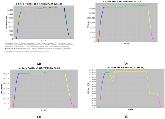
Figure 3.
The phases for two indicative flights as provided by DYNAMO (a,c) and as computed by the pre-processing method (b,d): (a) shows in detail all phases, as indicated by DYNAMO. The case shown in (b) is a good estimation compared to what DYNAMO specifies, but the case shown in (d) shows an incorrect estimation of flight phases compared to what is specified by DYNAMO, as shown in (c).
Therefore, the flight plans’ (DYNAMO_FP) dataset results in two distinct datasets, which are distinguished by the set of variables per trajectory point: One with trajectory variables provided by DYNAMOoptimization, and the other with trajectory variables provided by the pre-processing method. Both datasets are being used for training/testing distinct AI/ML models, although the later one is the one closer to operational conditions. The next section specifies the variables provided per dataset for the estimation of hidden parameters.
2.3. Problem Formulation
The goal is the estimation of the hidden parameters, CI and PL, given a flight plan and trajectory variables (in our case, either those provided by DYNAMOoptimization or those provided by the pre-processing module). This can be cast as a regression problem that targets the prediction of a vector of parameters Y, given a vector of input variables X.
In other words, the aim is to approximate a function f, such that:
where e constitutes a noise term or represents imperfections on data.
Y = f(X) + e,
In our case, the vector Y is a one- or two-dimensional output variable that corresponds to one or, respectively, two hidden parameters, while X is a feature vector that is derived from either the 11 variables that enrich each point of DYNAMO_FP trajectories (denoted as DYNAMO_FP(11) trajectories), shown in Table 1, or from the 8 variables that enrich each point of pre-processed DYNAMO_FP trajectories (denoted as DYNAMO_FP(8) trajectories), shown in Table 2.

Table 1.
Trajectory variables for DYNAMO_FP(11).
Table 2.
Trajectory variables for DYNAMO_FP(8).
According to the proposed methodology, the values of hidden parameters are known for the example trajectories provided for training. The goal is to learn models that generalize beyond the training dataset, approximating the function f(X) to estimate the values of hidden parameters of (unseen) trajectories with features X.
It must be noted that AI/ML methods for the estimation of both CI and PL do not take as input the variables specified in Table 1 and Table 2, but features derived from all these variables. Thus, for instance, absolute position variables are not used in their raw form, and thus estimations do not depend on them. This is specified subsequently in relation to each of the methods.
2.4. AI/ML Methods
This section provides a description of the machine-learning methods proposed to estimate the hidden parameters CI and PL. In conjunction with that, it specifies the trajectory features exploited and control variables involved in the validation exercises per method.
2.4.1. Graph Convolutional Network (GCN)
Using this method, inspired by [], the variables’ estimation problem is simulated as a decision of collaborative agents, each performing a regression task. This is an ensemble method, where homogeneous (i.e., sharing the same model parameters) regressors (agents) reach their own predictions using their own local observations (perceived features) of the flight trajectory. Agents collaborate to reach a joint decision regarding the estimation of variables. Collaboration results through communication of agents taking advantage of the neighboring relation. Agents are specified to be neighbors when their observations overlap, i.e., when they are related to the same or overlapping parts of the trajectory, or when their observations are from subsequent parts of the trajectory. In so doing, neighbor agents may have complimentary observations for the same part of the trajectory, or they may each have observations from a distinct part of the trajectory. The communication of agents is imprinted on a social adjacency graph with the connection of neighbor agents’ respective nodes via edges. The connectivity between agents is part of the method’s configuration, and subsequently we discuss these different options.
The intuition behind the interaction of neighboring agents is the conviction that they interplay with and affect each other towards predicting the values of the hidden parameters, taking advantage of their own and neighbors’ observations. Therefore, the specification of the agents’ (a) individual observations and (b) the adjacency matrix are crucial to the efficacy of the method.
To specify these aspects, the trajectory can be segregated into different parts, either vertically, corresponding for instance to the different flight phases or to more arbitrary parts of the flight; or horizontally, where each part incorporates few of the features regarding the whole flight trajectory. These options can be combined, so there are several alternatives to segregate trajectories. In any case, each agent gets as input its own/local observations from its corresponding part of the trajectory.
Having said that, we must clarify that this method, as well as all methods reported in [], do not consider the sequential nature of the trajectory, but they do consider the trajectory as a whole entity, whose features determine the values of hidden parameters.
To decide on agents, local agents’ observations and their adjacency relation, preliminary experiments have shown that having agents taking observations from distinct phases, and defining the agents’ neighbors according to the adjacency of flight phases, provides the best results. We conjecture that this happens due to the fact that hidden parameters play a definite role in shaping the vertical and lateral profiles of the trajectory in distinct flight phases. Specifically, the proposed method comprises three agents, each corresponding to a distinct flight phase (climbing, cruising and descent) as defined by DYNAMO_FP trajectories or as estimated by pre-processing those trajectories, respectively. The neighbors of an agent are those agents corresponding to phases that are adjacent to the phase of the agent. To provide agents with local observations, the corresponding sub-trajectories for the distinct flight phases are identified, and each flight phase is split into three parts, exploiting the aircraft altitude, as follows: Given that the altitude for a specific trajectory phase ranges in [a, b], each trajectory point is assigned to one of d classes, where each class c in {1, …, d} contains points with altitude values in the interval [a + (δ − 1) × c, a + δ × c), where δ = abs(b − a)/d.
The features computed per class are the mean and IQR (Q3 − Q1) for each of the variables in trajectory points.
Setting d = 3, this results, for the DYNAMO_FP(11) trajectories, in [11(variables) × 2(features per variable) × 3(phase parts)] features provided to each of the three agents as local observations, together with the total duration of each of the three phase parts, i.e., 69 features. Accordingly, for the DYNAMO_FP(8) trajectories, each agent gets [8(variables) × 2(features per variable) × 3(phase parts)] features, together with the total duration of each of the three phase parts, i.e., 51 features.
The overall architecture of this method is shown in Figure 4. The architecture of each agent (shown in Figure 4, bottom up) comprises an MLP encoder, two convolution layers and a dense regression layer whose outputs are the values of the hidden variables.
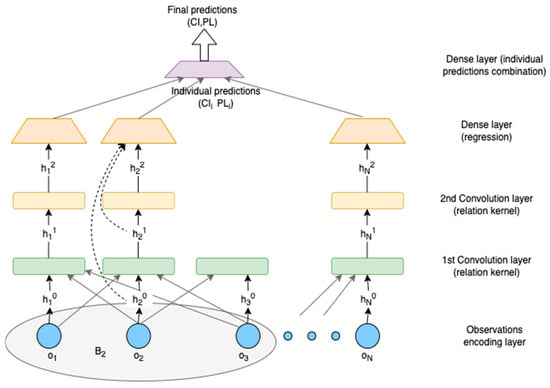
Figure 4.
The overall GCN method.
The proposed Graph Convolutional Network (GCN) method receives as input a feature matrix F, N × L, where N is the number of agents and L is the number of features provided as agents’ local observations o, together with an N × N adjacency matrix A(i, j), representing agents’ social graph G = (V, E), where V denotes the set of nodes corresponding to agents and E the set of edges connecting neighbor agents. Subsequently, the set of agent’s i neighbors is denoted as Bi.
According to Figure 4, the agent’s i local observations oi are passed through the encoding layer. The encoded observations hi0 with the adjacency matrix are provided to the first convolution layer. In addition, this layer gets as input the encoded observations hj0 from each agent j in Bi, increasing the agent’s i receptive field. This is a first round of agents’ communication. The output of the agent’s i first convolution layer is an updated feature vector hi1 provided to the second convolution layer, together with the output of agents’ j in Bi first-level convolution layer output hj1. In doing so, after this second round of communication, agents get information about 2-degrees neighbors and further increase their receptive field. We may add more layers, but two are sufficient, also given the small G we consider in our problem setting.
Convolution layers with multi-head dot-product attention kernels abstract the interactions (relations) among agents and extract high-order relation representations encoded into the latent features. This is important to the efficacy of the method, given that each agent learns to pay attention to observations from those parts of the trajectory (flight phases) that play important roles to its estimation concerning the values of hidden parameters.
To compute the attention values per head m in M = {0, 1, 2}, with j in B+i, i.e., including agent i and its neighbors, hi is projected to a query Qi, key Ki, and value Vi of equal size, which are split into M heads, of equal size, denoted by Qim, Kim, Vim, m = 1, …, M. The attention value of the m-th head is computed as follows:
where τ is a scaling factor, and and are m-th attention head trainable weights that project inputs into query and key matrices, respectively.
The output of the convolution procedure is computed as follows:
where σ is the activation function, i.e., one layer MLP with Rectified Linear Units (ReLUs), hi is the output of the convolutional layer i, and Wm denotes m-th attention head trainable value weights.
The dense regression layer receives as input the output of the two convolution layers and the encodings of the agent’s own observations to perform a regression task for the prediction of hidden variables’ values. This produces agents’ individual predictions, which are then combined at the last dense layer to provide the final estimation of hidden variables.
The control variables for the GCN are (a) the number of agents and the local observations per agent (which depend on how the trajectory is segregated), (b) the number of epochs, (c) the batch size, (d) the learning rate, as well as the (e) optimizer used and the configuration of (f) the MLP and of (g) the dense regression layers, i.e., number of layers, units and activation functions.
2.4.2. Gradient-Boosting Method (GBM)
Gradient-boosting trees are a machine-learning technique for optimizing the predictive value of a model through successive steps in the learning process. This is one of the methods studied in our previous work [], providing the best results for the estimation of hidden parameters. Here, we provide some background on this method, as it serves as the baseline with which GCN is compared with.
Typically, a decision tree is used as the basic weak machine-learning model, which makes decisions based on a series of rules that are organized in a tree shape. The gradient-boosting method (GBM) works in a stage-wise manner, iteratively adding a tree that aims to correct the errors of prior trees and then combining all trees in a weighted average to make the final prediction. The advantage of boosting methods is that the new model that is being added focuses on correcting the mistakes of the previous models. In contrast, other ensemble methods train the models in isolation, and this might simply lead to each model making the same mistakes.
For this method, our incentive is to manage each DYNAMO trajectory as a set of 1 − d representative features instead of a multi-dimensional sequence. Therefore, the features for DYNAMO(11) trajectories comprise the following ones: The median and the interquartile range (IQR, Q3 − Q1) per flight phase, for each of the 11 variables presented in Table 1, and the duration of each flight phase, which results in 3 additional features. This results in [11(variables) × 2(features per variable) × 3(phases) + 3], i.e., 69 input features representing the whole trajectory and a dependent output vector of two values: CI and PL. For DYNAMO(8), respectively, it results in [8(variables) × 2(features per variable) × 3(phases) + 3], i.e., 51 input features per trajectory.
The control variables in this case are: (a) the number of boosting stages to perform, denoted as n_estimators; (b) the minimum number of samples required at a leaf node, denoted as min_samples_leaf; (c) the minimum number of samples required to split an internal node, denoted as min_samples_split; (d) the maximum depth of the individual regression estimators that limits the number of nodes in a tree, denoted as max_depth; and (e) the learning_rate. The variables (b), (c) and (d) are considered tree-specific parameters in terms of ensemble modeling, as they affect each individual tree structure in the model, while (a) and (b) are the boosting parameters, as they affect the boosting operation.
3. Results
3.1. Experimental Setting
Every flight plan comprises approx. 600 points, and every such point is enriched with the trajectory variables shown in Table 1 for DYNAMO_FP(11) and in Table 2 for DYNAMO_FP(8). These variables are used for the calculation of the corresponding features, as specified in Section 2.4.
The two trajectory datasets have been split into training and testing subsets. Given 68 ALLFT+ M1 trajectories chosen for the purposes of validating trajectory modeling methods (not described in this paper) and given all possible combinations of CI and PL values for these flights, there are approx. 15700 DYNAMO_FP trajectories that have been used to test the hidden parameters’ estimation methods.
Τhe loss function considered is the mean absolute error (MAE). The results for DYNAMO_FP(11) and DYNAMO_FP(8) datasets are provided separately. This also serves the purpose of estimating the delta between estimated parameters using (a) flight plans enriched with all the variables provided by optimization methods, against (b) real-world flight plans whose variables are provided by pre-processing (approximation) methods.
The input features were scaled to the [0, 1] interval, while the estimated hidden parameters were left unscaled. Experiments showed that scaling CI and PL made no difference in estimating the hidden parameters, while scaling the input was mandatory for almost all methods. Finally, the models’ estimations were rounded to the closest integer for CI and to the 1st decimal position for PL.
The control variables’ values per method are specified in Table 3.
Table 3.
AI/ML methods’ parameters.
3.2. Experimental Results
The experimental results of all methods using the test set of DYNAMO_FP(11) trajectories are presented in Table 4, and those using the test set of DYNAMO_FP(8) trajectories are presented in Table 5. These tables show the performance of the two methods in terms of MAE in all DYNAMO_FP test trajectories. Numbers in bold indicate the best reported score.
Table 4.
Performance of AI/ML methods in DYNAMO_FP(11).
Table 5.
Performance of AI/ML methods in DYNAMO_FP(8).
Specifically, the results report the following quantities per method:
- MAE value (mean),
- MAE standard deviation (std),
- Interquartile MAE range IQR = Q3 − Q1,
- MAE range (max–min).
The results are also shown in Figure 5 and Figure 6 using boxplots. These figures show the MAE values (y-axis) for the CI variable (left) and PL variable (right) for each of the AI/ML methods used, indicated in the x-axis.
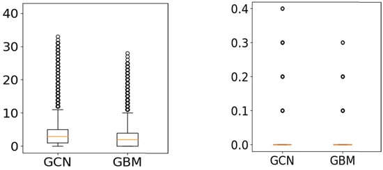
Figure 5.
Boxplots of results for DYNAMO(11). The Y axis corresponds to the MAE of the hidden parameters’ estimation (left: CI (kg/min), right: PL), and the X axis indicates the ML method used.
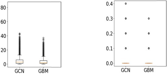
Figure 6.
Boxplots of results for DYNAMO(8). The Y axis corresponds to the MAE of the hidden parameters’ estimation (left: CI, right: PL), and the X axis indicates the ML method used.
From the results obtained, we can conclude that both methods achieve a good balance in estimating CI and PL in all cases. GBM manages to estimate CI more accurately in both datasets with a small std (thus exhibiting robustness and stability). It reports an MAE below 4% for CI and approx. 2% for PL. This concludes that GBM is very competitive, and the mean absolute error reported for CI is less than two times the discretization interval of the CI values provided in the training data (actually, 1.8 times the discretization interval, which is equal to 2), or less than 4%. Regarding PL, GBM reports results whose mean is much less than the discretization interval of the values provided in the training data (actually, 0.11 of the discretization interval, which is equal to 0.2), or less than 0.002% (i.e., 0.2 units in [0, 1]). However GCN manages to report nearly the same or even lower (in the case of DYNAMO_FP(8)) mean error for the estimation of PL. This is important given that DYNAMO_FP(8) cases are closer to reality and given the effect of PL in estimating important KPIs (discussed subsequently).
Also, the results show that both methods show consistent behavior when trained and tested using the features provided by DYNAMO and when trained and tested using the features provided by the pre-processing methods.
GCN reports results that are very close to those of GBM for the prediction of CI (the MAE differs by 0.8 units), while they are nearly the same or better (in the case of DYNAMO_FP(8)) for the prediction of the PL.
This shows that GBM and GCN can be used for the estimation of hidden parameters for real-world flight plans, even if variables are approximated by pre-processing methods. Additionally, studying the effects of their estimations on the prediction of KPIs reveals interesting results due to subtle issues regarding the accuracy of estimating hidden variables, which are discussed in the following section.
4. Discussion
This section reports on how the estimations of hidden parameters provided by the trained models support the prediction of flights’ KPIs using standard prediction error metrics (i.e., MAE). As already specified in the introduction, the KPIs are fuel consumption, flown distance, and gate-to-gate time.
To study the effects of hidden parameters’ estimation on KPIs’ prediction, we provide the results for the flight plans with known hidden parameters’ values. In this case, where hidden parameters’ values are known, the aim is to study how the difference between known and estimated values of the hidden parameters is reflected in differences between predicted and actual KPIs. Predicted KPIs are those that are provided by DYNAMOprediction considering the estimated values of hidden parameters, and true KPIs are those provided by DYNAMOprediction considering the known values of hidden parameters per trajectory. Actually, the comparison is between KPIs predicted using estimated hidden parameters and true KPIs computed using the actual values of hidden parameters, all provided by DYNAMOprediction.
The hidden parameters’ prediction models, i.e., GBM and GCN, are used to estimate the hidden parameters of the DYNAMO_FP(8) test trajectories. We consider the trajectories in the test set of DYNAMO_FP(8) only, since this is closer to the real-world case of model deployment. The overall comparison process described is shown in Figure 7.
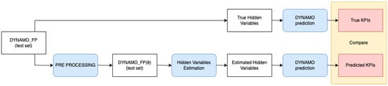
Figure 7.
The process for estimating the effect of hidden parameters’ estimation errors on the prediction of KPIs.
Given that DYNAMOprediction predictions for flown distance and gate-to-gate time do not differ when DYNAMOprediction considers the true or the estimated values of parameters, below we report only differences regarding the fuel consumption prediction.
Table 6 shows the effect of hidden parameters’ estimation errors on the predictions of fuel consumption: rows correspond to absolute differences in estimating CI, columns correspond to absolute differences in estimating PL, the values in cells show the mean absolute percentage of error (MAPE) in the fuel consumption prediction for all cases with the corresponding differences in CI and PL. In addition, each cell reports the percentage of testing cases with the corresponding CI and PL errors. The results show that both hidden parameters conjunctively play a role in fuel consumption estimation. However, PL plays a more critical role: large errors in PL are translated into large differences in predicted fuel consumption.
Table 6.
The effect of hidden parameters’ estimation errors on the prediction of fuel [kg]: Rows correspond to absolute differences in estimating CI, columns correspond to absolute differences in estimating PL, and each cell indicates two values: (a) the mean absolute percentage error of predicted vs. actual fuel for all trajectories with the corresponding differences in CI and PL, and (b) the percentages of trajectories with those CI and PL differences. N/A means there were no cases with this combination of CI and PL absolute differences. Colors indicate the magnitude of error on the prediction of fuel: Light (dark) color indicate small (resp. large) error.
It is interesting to note that although GCN scores a slightly worst performance compared to GBM in relation to the prediction of hidden variables, it results in a better prediction of fuel consumption on average.
Delving into the results, we can observe the following facts: (a) Considering the absolute differences in predicted vs. true PL, although GBM does not result in an MAE larger than 0.3 for the prediction of PL, GCN reports 0.07% test cases with an MAE equal to 0.4 for PL and an MAPE for fuel consumption of approximately 6.5, while (b) GCN encounters more test cases that result in a smaller MAPE for predicted fuel consumption compared to GBM for differences in the prediction of PL of less than 0.4. Finally, the test cases with small differences in predicted PL (i.e., in columns 0 and 0.1) are more for GCN compared to the respective cases of GBM, and most of these cases score a small absolute difference in the prediction of CI, in the range of 0–9. Overall, these facts show a distribution of test cases into classes of PL/CI estimation errors, which results in a lower expected error for GCN compared to GBM regarding the estimation of fuel consumption.
This is shown in Table 7, which reports on the weighted average score for predicting fuel consumption using estimated parameters from both methods, per absolute difference of predicted vs. true PL and predicted vs. true CI. Numbers in bold indicate the best scores. Weighted average scores are computed by averaging the weighted sum of absolute differences in fuel prediction, where percentages of cases providing the difference in prediction serve as weights. The results show that on expectation GCN is considerably better than the other methods in the prediction of fuel consumption considering either the errors in the predicted CI or the errors in the predicted PL.
Table 7.
Weighted average score of methods in predicting fuel consumption.
Furthermore, as Figure 8 shows, the distributions of fuel consumption in all cases, either with the estimated hidden parameters or with the true hidden parameters, are the same, and this occurs (following a t-test on these predictions) with a probability 0.99.
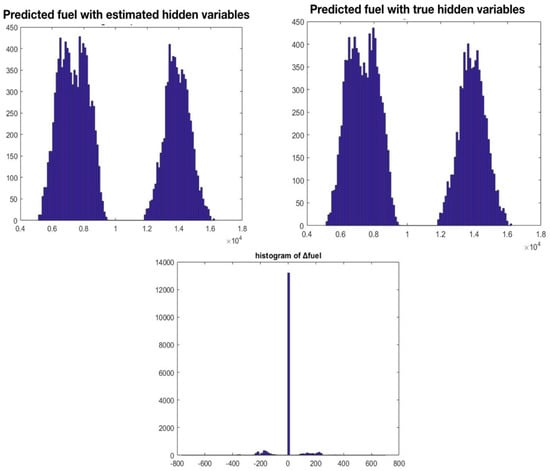
Figure 8.
The distributions of predicted fuel consumption [kg] given the estimations of hidden parameters (top left) and the true hidden parameters (top right), as well as the distribution of the absolute difference in the predicted fuel (bottom).
The above results verify the efficacy of the hidden parameters’ estimation methods GCN and GBM in supporting the prediction of trajectory-related KPIs. The MAPE for fuel consumption is below 1%, while for flown distance and gate-to-gate-time it is 0%. Therefore, we can conclude that the proposed AI/ML methods for the estimation of hidden parameters support the prediction of trajectory KPIs with a high accuracy, with GCN supporting the more accurate predictions in expectation.
This result also provides firm evidence of the hypothesis that the reported hidden parameters’ estimation errors have insignificant consequences on the prediction of KPIs. This is especially important since it demonstrates that the methodology is robust against the high cruise ECON Mach sensitivity to fuel flow (or specific range) variations. As reported in [], due to the flat nature of the specific range curve near the Maximum Range Cruise and Long Range Cruise optimum speeds, cruise ECON Mach can significantly vary for low CI values, depending on the actual accuracy of the aircraft performance model used. Hence, the method proposed in this paper is particularly useful for obtaining aggregated KPIs to address ATM performance, even if the aircraft performance model is not directly derived from OEM (original equipment manufacturer) data, such as the BADA model.
5. Conclusions
This paper explores the use of machine-learning techniques for the estimation of flights’ hidden parameters from historical data. Specifically, it presents a data-driven methodology for the estimation of flights’ hidden parameters, combining mechanistic and AI/ML models. In the context of this methodology, the paper proposes and evaluates AI/ML methods to estimate payload mass and cost index. In addition, the paper examines how these estimations affect the prediction of KPIs regarding the efficiency of flights: fuel consumption, gate-to-gate time and distance flown. The results show the accuracy of the proposed methods and the benefits of the proposed methodology.
Future work aims to explore (a) the use of different prediction and optimization mechanistic models for the purposes of the proposed methodology, (b) alternative configurations for GCN, so as to identify agents and their neighbors using different chunks of trajectories, (c) the concurrent use of multiple configurations, as well as (d) other deep AI/ML methods for the estimation of hidden parameters in conjunction with the estimation of other hidden variables enriching trajectories.
Author Contributions
Conceptualization, G.V. and X.P.; methodology, X.P. and G.V.; software, I.I., T.T., G.V. and K.B.; validation, I.I., T.T. and K.B.; resources, G.V., X.P., M.M. and G.S.; writing—original draft preparation, G.V. and T.T.; writing—review and editing, all authors; visualization, T.T.; supervision, G.V. and X.P.; project administration, G.V. and X.P.; funding acquisition, G.V. and X.P. All authors have read and agreed to the published version of the manuscript.
Funding
This work has received funding from SESAR Joint Undertaking (JU) within the SIMBAD project under grant agreement ID 894241. The JU receives support from the European Union’s Horizon 2020 research and innovation programme and SESAR JU members other than the Union.
Data Availability Statement
The DYNAMO_FP datasets presented in the study, as well GCN and GBM implementations, will be made openly available in [repository name, e.g., FigShare] at [DOI/URL] when this article is accepted for publication.
Conflicts of Interest
The authors declare no conflicts of interest. The funders had no role in the design of the study; in the collection, analyses, or interpretation of data; in the writing of the manuscript; or in the decision to publish the results.
References
- ICAO. Manual on Air Traffic Management System Requirements, 1st ed.; ICAO: Montreal, QC, Canada, 2008. [Google Scholar]
- ICAO. Manual on Global Performance of the Air Navigation System, 1st ed.; ICAO: Montreal, QC, Canada, 2009. [Google Scholar]
- CANSO. Recommended Key Performance Indicators for Measuring ANSP Operational Performance; Technical Report; CANSO: Utrecht, The Netherland, 2015. [Google Scholar]
- European Commission. Commission Implementing Regulation (EU) No 390/2013 of 3 May 2013; European Union: Brussels, Belgium, 2015. [Google Scholar]
- APACHE Consortium. Review of Current KPIs and Proposal for New Ones. APACHE Project, Technical Report D3.1 v02.00.00. July 2018. Available online: http://hdl.handle.net/2117/114127 (accessed on 12 September 2024).
- RTCA. Measuring NextGen Performance: Recommendations for Operational Metrics and Next Steps; Technical Report BCPMWG; AIRBUS S.A.S: Blagnac, France, 2011. [Google Scholar]
- FAA. NextGen Performance Snapshots Reference Guide. 2017. Available online: https://www.faa.gov/sites/faa.gov/files/2021-11/FAA_Report_to_Congress_on_NextGen_Performance_Metrics.pdf (accessed on 12 September 2024).
- Zhang, H.; Xu, Y.; Yang, L.; Liu, H. Macroscopic Model and Simulation Analysis of Air Traffic Flow in Airport Terminal Area; Forward Series; Wiley Online: New Jersey, NJ, USA, 2014. [Google Scholar]
- Grether, D.; Furbas, S.; Nagel, N. Agent-based Modelling and Simulation of Air Transport Technology. Procedia Comp. Sci. 2013, 19, 821–828. [Google Scholar] [CrossRef][Green Version]
- Delgado, L.; Gurtner, G.; Mazzarisi, P.; Zaoli, S.; Valput, D.; Cook, A.; Lillo, F. Network-wide assessment of ATM mechanisms using an agent-based model. J. Transp. Manag. 2021, 95, 102108. [Google Scholar] [CrossRef]
- Airbus. Getting to Grips with the Cost Index-Issue II; Technical Report, Flight Operations Support & Line Assistance; Radio Technical Commission for Aeronautics: Washington, DC, USA, 1998. [Google Scholar]
- Prats, X.; Dalmau, R.; Barrado, C. Identifying the sources of flight inefficiency from historical aircraft trajectories. A set of distance- and fuel-based performance indicators for post-operational analysis. In Proceedings of the 13th USA/Europe Air Traffic Management Research and Development Seminar, Vienna, Austria, 17–21 June 2019; Eurocontrol and FAA: Vienna, Austria, 2019. [Google Scholar]
- Feng, T.; Timmermans, H.J. Comparison of advanced imputation algorithms for detection of transportation mode and activity episode using GPS data. Transp. Plan. Tech. 2016, 39, 180–194. [Google Scholar] [CrossRef]
- Hernández, Y.; Djukic, T.; Casas, J. Local traffic patterns extraction with network-wide consistency in large urban networks. Transp. Res. Procedia 2018, 34, 259–266. [Google Scholar] [CrossRef]
- Antunes, F.; Amorim, M.; Pereira, F.C.; Ribeiro, B. Active learning metamodeling for policy analysis: Application to an emergency medical service simulator. Simul. Model. Pract. Theory 2019, 97, 101947. [Google Scholar] [CrossRef]
- COPTRA Consortium. COPTRA Deliverable D2.1. Techniques to Determine Trajectory Uncertainty and Modelling. Technical Report, Edition 01.00.00. 2017. Available online: https://www.researchgate.net/publication/317091485_COPTRA_D21_Techniques_to_determine_trajectory_uncertainty_and_modelling (accessed on 12 September 2024).
- SIMBAD. Combining Simulation Models and Big Data Analytics for ATM Performance Analysis. Available online: https://www.sesarju.eu/projects/SIMBAD (accessed on 12 September 2024).
- Alligier, R.; Gianazza, D. Learning aircraft operational factors to improve aircraft climb prediction: A large scale multi-airport study. Transp. Res. Part C Emerg. Technol. 2018, 96, 72–95. [Google Scholar] [CrossRef]
- Alligier, R.; Gianazza, D.; Durand, N. Machine Learning and Mass Estimation Methods for Ground-Based Aircraft Climb Prediction. IEEE Trans. Intell. Transp. Syst. 2015, 16, 3138–3149. [Google Scholar] [CrossRef]
- Gheorghe, A.I. Prediction of Aircraft Take-Off Weight using Machine Learning. MSc Thesis, TU Delft, Delft, The Netherlands, 2024. Available online: https://resolver.tudelft.nl/uuid:3a2b3d2e-e4f3-4042-9172-f03ccc67cda1 (accessed on 12 September 2024).
- Tranos, T.; Vouros, G.A.; Blekas, K.; Santipantakis, G.; Melgosa, M.; Prats, X. Data driven estimation of flights’ hidden parameters. In Proceedings of the 12th SESAR Innovation Days (SIDs), Budapest, Hungary, 5–8 December 2022. [Google Scholar]
- He, X.; He, F.; Zhu, X.; Li, L. Data-driven Method for Estimating Aircraft Mass from Quick Access Recorder using Aircraft Dynamics and Multilayer Perceptron Neural Network. arXiv 2020, arXiv:2012.05907. Available online: https://api.semanticscholar.org/CorpusID:228376122 (accessed on 12 September 2024).
- Chati, Y.S.; Balakrishnan, H. Statistical modeling of aircraft take-off weight. In Proceedings of the 12th USA/Europe Air Traffic Management Research and Development Seminar, Berkeley, CA, USA, 27–30 June 2017. [Google Scholar]
- Sun, J.; Ellerbroek, J.; Hoekstra, J. Modeling and Inferring Aircraft Takeoff Mass from Runway ADS-B Data. June 2016. Available online: https://www.researchgate.net/publication/305403975_Modeling_and_Inferring_Aircraft_Takeoff_Mass_from_Runway_ADS-B_Data (accessed on 12 September 2024).
- Sun, J.; Blom, H.A.; Ellerbroek, J.; Hoekstra, J.M. Particle filter for aircraft mass estimation and uncertainty modeling. Transp. Res. Part C Emerg. Technol. 2019, 105, 145–162. Available online: https://api.semanticscholar.org/CorpusID:197454207 (accessed on 12 September 2024). [CrossRef]
- Sun, J.; Ellerbroek, J.; Hoekstra, J. Bayesian Inference of Aircraft Initial Mass. June 2017. Available online: https://www.researchgate.net/publication/317600026_Bayesian_Inference_of_Aircraft_Initial_Mass (accessed on 12 September 2024).
- Sun, J.; Ellerbroek, J.; Hoekstra, J.M. Aircraft initial mass estimation using Bayesian inference method. Transp. Res. Part C Emerg. Technol. 2018, 90, 59–73. [Google Scholar] [CrossRef]
- Dalmau, R.; Melgosa, M.; Vilardaga, S.; Prats, X. A Fast and Flexible Aircraft Trajectory Predictor and Optimiser for ATM Research Applications. In Proceedings of the ICRAT 2018—8th International Conference for Research in Air Transportation, Castelldefels, Espanya, 26–29 June 2018; pp. 1–8. Available online: http://hdl.handle.net/2117/122638 (accessed on 12 September 2024).
- Jiang, J.; Dun, C.; Huang, T.; Lu, Z. Graph Convolutional Reinforcement Learning. arXiv 2018, arXiv:1810.09202. [Google Scholar]
- Kingma, D.P.; Ba, J. Adam: A Method for Stochastic Optimization. arXiv 2014, arXiv:1412.6980. [Google Scholar]
- Mouillet, V.; Nuić, A.; Casado, E.; López Leonés, J. Evaluation of the Applicability of a Modern Aircraft Performance Model to Trajectory Optimization. In Proceedings of the 2018, IEEE/AIAA 37th Digital Avionics Systems Conference (DASC), London, UK, 23–27 September 2018; pp. 1–10. [Google Scholar] [CrossRef]
Disclaimer/Publisher’s Note: The statements, opinions and data contained in all publications are solely those of the individual author(s) and contributor(s) and not of MDPI and/or the editor(s). MDPI and/or the editor(s) disclaim responsibility for any injury to people or property resulting from any ideas, methods, instructions or products referred to in the content. |
© 2024 by the authors. Licensee MDPI, Basel, Switzerland. This article is an open access article distributed under the terms and conditions of the Creative Commons Attribution (CC BY) license (https://creativecommons.org/licenses/by/4.0/).