Article

Adaptive Robust Time-Varying Formation Control of Quadrotors under Switching Topologies: Theory and Experiment

1
School of Aeronautic Science and Engineering, Beihang University, Beijing 100191, China
2
Institute of Unmanned System, Beihang University, Beijing 100191, China
*
Author to whom correspondence should be addressed.
Aerospace 2023, 10(8), 735; https://doi.org/10.3390/aerospace10080735
Submission received: 30 June 2023 / Revised: 14 August 2023 / Accepted: 15 August 2023 / Published: 21 August 2023

Abstract

:
This paper investigates a practical time-varying formation control method for quadrotors subjected to disturbances, uncertainties, and switching-directed topologies. A fully distributed formation control scheme is proposed using a linear-velocity independent position controller (LVIPC) and a nonsingular terminal sliding mode attitude controller (NTSMAC). A distributed observer is adopted to eliminate the measurement of linear-velocity states, and only local neighbor states are needed to realize formation flight. A time-varying nonsingular terminal sliding mode manifold is designed to suppress the reaching phase and ensure the finite-time convergence. Adaptive estimators are employed to remove the reliance on the prior knowledge of the upper bound of lumped uncertainties. It is then proven that all the closed-loop signals are bounded under the proposed method. Comparative experimental results based on a practical outdoor hardware solution are presented to confirm the effectiveness of the suggested control algorithm.

1. Introduction

In recent years, the formation control technology of unmanned aerial vehicles (UAVs) has received widespread attention. Compared to a single UAV, a formation of multiple UAVs has greater application efficiency and enormous potential in the aerospace domain due to its capacity for aerial environmental surveillance, cooperative remote sensing, and even military applications [1,2,3].
As a typical small UAV, a quadrotor (QR) has advantages such as its light weight, simple structure, maneuverability, and hovering capability [4], making it an ideal platform for formation control. Due to its well-known under-actuation, strong coupling, and nonlinear characteristics [5], the QR system can be transformed into a dual-loop structure. However, the position control (outer-loop) highly relies on attitude tracking (inner-loop) [6], which makes control design challenging. Nevertheless, most existing results on QR formation control assumed that QR has an attitude autopilot [7,8,9] and only focuses on the position control design. The few studies that involved attitude control usually adopted simplified models under the “small-angle approximation” assumption [10,11,12], which narrows the application scope. Moreover, in practical application, environmental disturbances and system uncertainties heavily impact QR’s flight, with the attitude control system being particularly sensitive to these effects [13]. Therefore, a robust attitude controller based on a full nonlinear model is critical for QRs to achieve the desired formation flight. A variety of robust control strategies have been studied recently, including H- control [14,15], sliding mode control (SMC) [16,17], super-twisting control [18,19], and integral backstepping control [20,21]. Among these, SMC is widely used in the control of satellites, aircrafts, and robots owing to its fast response, easy implementation, and robustness. Nevertheless, conventional SMC based on linear hyperplanes can only guarantee asymptotic convergence [22,23]. In order to obtain finite-time convergence, the nonlinear hyperplane-based terminal sliding mode (TSM) and its variants—the nonsingular terminal sliding mode (NTSM) and the fast nonsingular terminal sliding mode (FNTSM) techniques—have emerged. In [24], the finite-time tracking control of a QR under input delay, uncertainty, and disturbance was addressed by combining NTSM with adaptive laws. In [25], adaptive super-twisting NTSM tracking control was designed for a QR with bounded disturbances to decrease the chattering phenomena. In [26,27], adaptive FNTSM controllers were adopted to ensure the finite-time convergence of the QR’s attitude states subjected to disturbances. However, there are still obstacles and limitations to its practical application. Firstly, the system state is sensitive to disturbances and uncertainties during the reaching phase, before entering the sliding phase, which degrade the robustness of the system [28,29,30]. Secondly, these methods can only ensure that the convergence time is bounded but cannot be easily adjusted, which may cause inconvenience in engineering applications. To address these problems, a novel time-varying nonsingular terminal sliding mode (TVNTSM) manifold is adopted in this paper. To the best of our knowledge, the application of TVNTSM in formation control is still very scarce [31,32,33].
The role of the formation position controller of the QR is to exchange information with neighboring QRs, to obtain the tracking error, and to generate the command signal for inner-loop and thrust. In the past few decades, owing to its scalability and distributed nature [34,35], the consensus theory has stood out from among various formation control approaches, including behavior-based [36,37], virtual structure [38,39], and leader-follower [40,41] approaches. In [42], the formation control of multiple QRs subjected to perturbations was executed with the use of a consensus error model and adaptive laws. In [43], modified model predictive control was applied to realize the formation flight of networked QRs subjected to disturbances. In [44], the predefined-time formation control for QR clusters was realized by employing the state observer and SMC. However, the formation pattern was time-invariant in these works. In practical applications such as target enclosing [45] and area coverage [46], the formation pattern needs to be adjustable in order to obtain a wider range of detection angles and to be able to capture more varied information. In [47], a PD-like controller was designed for the time-varying formation control (TVFC) of multiple UAVs with delays and uncertainties. In [48], the distributed finite-time TVFC of multiple QRs with aperiodic sampled data was studied. In [49], the neural adaptive TVFC of multiple QRs with faults was studied in a practical application. However, only fixed topology was adopted in the results. To maintain a reliable connection, the interconnection should be switchable to accommodate the varying distance between UAVs and possible signal blocking during the formation adjustment [50]. In [51,52,53], the eigenvalues of the Laplacian matrix of networks were required to achieve formation control. However, such global information is hard to obtain in large-scale formations [54]. In [55,56,57], the fully distributed schemes without global information were investigated. Nevertheless, these methods still have limitations. Firstly, in addition to position state, formation members also need to measure velocity state, which can be inaccessible due to the measure noise. Secondly, these methods lack practical flight verification, and most of the existing experimental results are based on indoor solutions such as motion capture systems or UWB positioning. However, these indoor experimental schemes cannot well reflect wind disturbance and other factors in outdoor natural environments. Therefore, outdoor experiments based on practical hardware is conducted in this paper.
Based on the above discussions, this paper investigates a fully distributed and adaptive robust time-varying formation control method for QRs with switching topology. Compared to existing research, the main contributions of this paper, both in theory and application, are as follows:
  • In terms of theory, firstly, for easy application, adaptive laws were adopted to remove the reliance on the prior knowledge of the unknown upper bound of lumped uncertainties. Secondly, the TVNTSM manifold was designed to suppress the impact of the reaching phase on system robustness and guarantee the convergence of the system state in adjustable finite time, thereby improving practicality. Thirdly, distributed observers were employed to eliminate the measurement of linear velocity, with the possibility of realizing formation control without any global topology information, thereby making it fully distributed. Fourthly, both formation pattern and directed topology could be dynamically adjusted, making it suitable for scenarios such as target enclosing, area coverage, and target tracking.
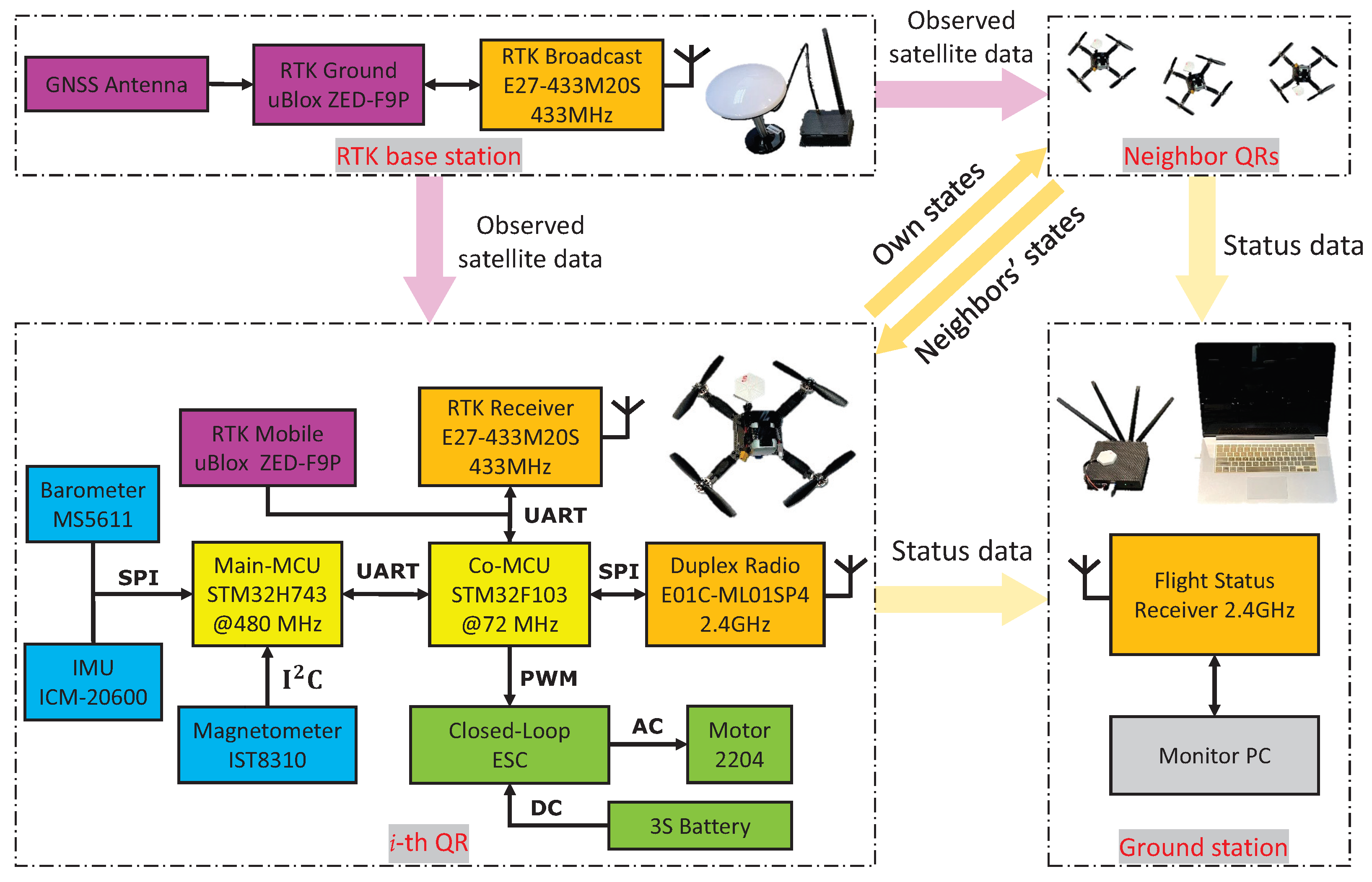
  • In terms of application, this study differs from most previous research that only conducted experimental verification in ideal indoor environments based on motion capture or UWB positioning. Instead, an outdoor scheme was designed for this study, with all QRs flying in natural disturbed environments. Their positions were provided by the RTK system in accordance with actual working conditions. In addition, unlike most previous research that relied on a robot operating system (ROS) with high hardware requirements or Wi-Fi with a limited range to establish the interconnection of UAVs, this paper utilized bi-directional wireless modules to build the QR network, such that total control could be achieved through micro control unit (MCU)-based hardware solutions, which is currently the mainstream solution used in the drone industry.

2. Preliminaries and Problem Formulation

2.1. Notations

Let a b denote the Kronecker product of matrices a and b , and λ m i n ( ) and λ m a x ( ) respectively indicate the minimum and maximum eigenvalues of a matrix. Let 0 denote the zero matrix with a proper size, and s ( ) and c ( ) denote sin ( ) and cos ( ) . I m denotes the m-dimensional identity matrix. denotes the absolute value of a real number, the Euclidean norm of a vector, and F the Frobenius norm of a matrix. Let ( ) k denote the k-th row of a matrix. For a vector X = [ X 1 , , X n ] T , let s i g β ( X ) = [ s i g β ( X 1 ) , , s i g β ( X n ) ] T with s i g β ( X i ) = X i β s i g n ( X i ) .

2.2. Graph Theory

A directed graph of N QR followers can be defined by G F = Q , E , A with the node set Q = q 1 , q 2 , , q N , the edge set E Q × Q , and the weighted adjacency matrix A . A = [ a i j ] R N × N is defined as a i j = > 0 , if ( q i , q j ) E , otherwise a i j = 0 . a i i = 0 for all i Σ = 1 , 2 , , N . The set of neighbors of the i-th QR is defined by N i = q j | ( q i , q j ) E . The Laplacian matrix of G F is denoted by L F = [ l i j F ] R N × N , with l i j F = a i j ( i j ) and l i i F = q j N i a i j . The total flight time interval of the QRs is defined as [ 0 , T t ) , which can be divided into an infinite sequence of bounded time intervals [ t p , t p + 1 ) ( p Π ) , where Π represents all natural numbers, with t 0 = 0 . The dwell time T d meets 0 < T d t p + 1 t p T t , and the graph is fixed during [ t p , t p + 1 ) . G A F is denoted as the set of all possible graphs, with the index set being Γ G A F Π . S ( t ) : R 0 + Γ G A F is defined as the switching signal. The follower graph, Laplacian matrix, and neighbor set of the i-th QR at time t are G S ( t ) F , L S ( t ) F , and N i S ( t ) , respectively. If the leader q 0 is a neighbor of the i-th QR at time t, then the connection weight b i = 1 , otherwise, b i = 0 . The whole graph of N QRs and the leader at time t is G S ( t ) , with the corresponding Laplacian matrix being L S ( t ) = 0 0 L S ( t ) L L S ( t ) F , where L S ( t ) L = [ b 1 , b 2 , , b N ] T . Let W S ( t ) = L S ( t ) + B S ( t ) , with B S ( t ) = d i a g b 1 , b 2 , , b N . If there is a node that has a path to all other nodes, it is said that G S ( t ) has a directed spanning tree.
Lemma 1. 
W S ( t ) is positive-definite when there is a directed spanning tree in G S ( t ) , with the leader q 0 being the root node.
Assumption 1. 
All the possible graphs of G S ( t ) have a directed spanning tree rooted at q 0 .

2.3. Problem Formulation

Consider N QRs following a leader, with their topology described by G S ( t ) . The nonlinear dynamics of the QR can be obtained as follows through Newton’s laws [58]:
P ˙ i = V i V ˙ i = g e 3 K i t V i + R i t T i m i e 3
η ˙ i = R i r Ω i J i Ω ˙ i + C i r Ω i + K i r Ω i = τ i + τ i d
where i Σ , P i = [ x i , y i , z i ] T , V i = [ v i x , v i y , v i z ] T , and η i = [ ϕ i , θ i , ψ i ] T are position, linear velocity, and Euler angle in an earth-fixed frame, respectively. Ω i = [ p i , q i , r i ] T represents the angular velocity in a body-fixed frame. m i and J i = d i a g J i x , J i y , J i z are the total mass and inertia matrix. T i denotes the total lift, e 3 = [ 0 , 0 , 1 ] T and g represent the gravity. K i t = d i a g K i x t , K i y t , K i z t and K i r = d i a g K i x r , K i y r , K i z r are the translational and rotational damping matrices, respectively. C i r = S ( Ω ) J i represents the Coriolis term. τ i = [ τ i 1 ,   τ i 2 ,   τ i 3 ] T and τ i d are control torque and disturbance acting on the QRs. R i t ,   R i r and S ( Ω i ) are expressed as follows:
R i t = c θ i c ψ i s θ i c ψ i s ϕ i s ψ i c ϕ i s θ i c ψ i c ϕ i + s ψ i s ϕ i c θ i s ψ i s θ i s ψ i s ϕ i + c ψ i c ϕ 1 s θ i s ψ i c ϕ i c ψ i s ϕ s θ i c θ i s ϕ i c θ i c ϕ i ,
R i r = 1 c θ i c θ i s ϕ i s θ i c ϕ i s θ i 0 c ϕ i c θ i s ϕ i c θ i 0 s ϕ i c ϕ i , S ( Ω i ) = 0 r i q i r i 0 p i q i p i 0 ,
In order to facilitate the subsequent control design, the attitude dynamics can be transformed from the body-fixed frame to the earth-fixed frame. Taking the time derivative of the kinetics part in (2), we have the following:
η ¨ = R ˙ i r Ω i + R i r Ω ˙ i
Combining (3) and the attitude dynamics in (2), we have:
J ¯ i A ¨ i + C ¯ i r A ˙ i + K ¯ i r A ˙ i = τ i + τ i d
where J ¯ i = J ¯ i 0 + Δ J ¯ i , C ¯ i r = C ¯ i r 0 + Δ C ¯ i r and K ¯ i r = K ¯ i r 0 + Δ K ¯ i r are the nominal and uncertain terms of the QR’s attitude model, with J ¯ i 0 = J i R i r 1 , C ¯ i r 0 = ( C i r J i R i r 1 R ˙ i r ) R i r 1 and K ¯ i r 0 = K i r R i r 1 . Then, (4) can be rewritten as follows:
J ¯ i 0 A ¨ i + C ¯ i r 0 A ˙ i + K ¯ i r 0 A ˙ i = τ i + d i
where d i = Δ J ¯ i A ¨ i Δ C ¯ i r A ˙ i Δ K ¯ i r A ˙ i + τ i d is the lumped uncertainty of the attitude system.
The pattern of the QR formation is defined by a vector Υ P ( t ) = [ Υ 1 T ( t ) , Υ 2 T ( t ) , , Υ N T ( t ) ] T , where Υ i ( t ) = [ Υ i 1 ( t ) , Υ i 2 ( t ) , Υ i 3 ( t ) ] T , i Σ , Υ i k ( t ) is the second-order differentiable motion mode function that defines the movement of the i-th QR with respect to the leader, k = 1 , 2 , 3 . The leader’s position and velocity are P 0 ( t ) = [ x 0 , y 0 , z 0 ] T and P ˙ 0 ( t ) = V 0 ( t ) = [ v 0 x , v 0 y , v 0 z ] T , and the bounded control input U 0 ( t ) = V ˙ 0 ( t ) of the leader is unknown to all follower QRs, thus satisfying U 0 ( t ) U M . Based on the consensus theory, the following definition is given:
Definition 1. 
The formation tracking is said to be achieved when
lim t ( P i P 0 Υ i ) = 0 , i Σ
The snap shots of a rotating formation with N = 3 at time t 1 , t 2 are shown in Figure 1 to illustrate Definition 1. One sees that if P i P 0 Υ i = 0 for i 1 , 2 , 3 , then the triangle P 1 P 2 P 3 would precisely be the expected pattern defined by Υ 1 , Υ 2 , Υ 3 , namely the formation pattern is formed. Then, the QRs will follow the leader P 0 along its trajectory to achieve formation tracking.

2.4. Control Objective

The objective of this paper is to enable, under the proposed TVFC method, the trajectory of the leader P 0 ( t ) to be tracked and the predefined time-varying formation pattern Υ P ( t ) to be formed by follower QRs subjected to uncertainties and disturbance in (5). The detailed control objectives are shown below:
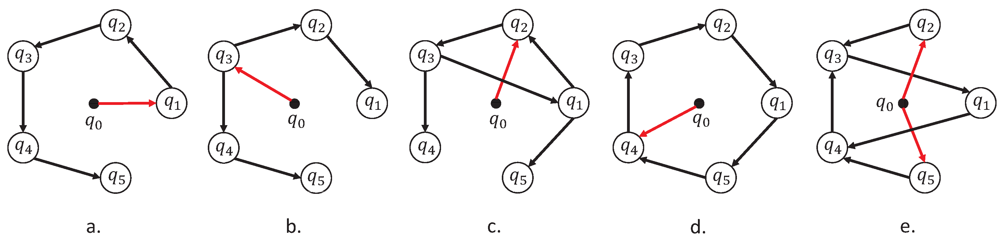
  • The QR’s formation pattern and directed topology can be dynamically adjusted under the fully distributed TVFC protocol;
  • The measurement and transmission of the QR’s linear-velocity can be eliminated by distributed observers;
  • The influence of the reaching phase can be suppressed by adopting TVNTSM, and the finite convergence time of the attitude tracking error can be adjusted;
  • The reliance on the prior knowledge of the unknown upper bound of lumped uncertainty d i can be removed by adaptive laws.

3. Main Results

The desired TVFC scheme can be divided into a linear-velocity independent position controller (LVIPC) and a nonsingular terminal sliding mode attitude controller (NTSMAC), as shown in Figure 2. The inputs of its outer-loop, including the local neighbor information ( P j , V ^ j ) j N i S ( t ) , leader information P 0 , and pattern vector Υ P were transferred to the LVIPC. Meanwhile, the linear velocity estimation value V ^ i was generated by the observer, and the global information was estimated by an adaptive coupling weight. Then, the output U i P of LVIPC was utilized to calculate the desired thrust T i C and command attitude signal ϕ i C , ψ i C . The inputs of the inner-loop, including ϕ i C , ψ i C , and ψ i C , were entered into the NTSMAC. Then, the attitude-tracking errors e i A and e i Ω were used to construct the TVNTSM manifold S i ( t ) and adaptive laws D i k m for lumped uncertainty rejection. Finally, T i C and the output τ i of NTSMAC were applied to the i-th QR for the TVFC.

3.1. Design of LVIPC

For each QR, the position and velocity tracking errors are constructed using the local neighbor’s information as follows:
e i P ( t ) = j N i S ( t ) a i j [ P i ( t ) P j ( t ) Λ i j ( t ) ] + b i ( P i ( t ) P 0 ( t ) Υ i ( t ) )
e i V ( t ) = j N i S ( t ) a i j [ V ^ i ( t ) V ^ j ( t ) Λ ˙ i j ( t ) ] + b i ( V ^ i ( t ) V 0 ( t ) Υ ˙ i ( t ) )
where Λ i j = Υ i Υ j , V ^ i is the estimation of the linear velocity of the i-th QR, which is given by an observer that needs to be designed later. Let E i ( t ) = e i P ( t ) + e i V ( t ) and regard the control input of the i-th QR’s position subsystem (1) as U i p ( t ) = g e 3 + R i t T i m i e 3 , and U i p can now be designed as follows:
U i P ( t ) = Φ G ( E i ( t ) ) W i ( t ) E i ( t ) + Υ ¨ i K i t V ^ i W ˙ i ( t ) = w i E i T ( t ) E i ( t )
where Φ U M is the gain constant, and the nonlinear function G ( E i ( t ) ) = E i ( t ) ( E i ( t ) + E 0 ) 1 , with E 0 > 0 , is a small constant. W i ( t ) is the adaptive law used to estimate the global information for the current graph G S ( t ) , with W i ( 0 ) > 0 . w i is a positive design parameter.
Then, the linear velocity observer is designed as follows:
V ^ i ( t ) = γ i ( t ) + Ψ ( P i Υ i ) γ ˙ i ( t ) = Ψ V ^ i ( t ) + U i P ( t ) + K i t V ^ i ( t ) + Ψ Υ ˙ i
where γ i ( t ) is the observer state, and Ψ > K ¯ t is a gain constant, with K ¯ t = m a x ( K i t F ) , i Σ .
Lemma 2. 
According to [59], the following three inequalities hold simultaneously for an asymmetric matrix ϖ = ϖ 11 ϖ 12 ϖ 12 T ϖ 22 : (1) ϖ 11 < 0 , ϖ 22 ϖ 12 T ϖ 11 1 ϖ 12 < 0 ; (2) ϖ 22 < 0 , ϖ 11 ϖ 12 ϖ 22 1 ϖ 12 T < 0 ; (3) ϖ < 0 .
Theorem 1. 
Under Assumption 1, along with the control law (9) and the observer (10), a group of N QRs described by position system (1) will form the desired time-varying formation pattern Υ P and track the leader along its trajectory P 0 ( t ) .
Proof. 
Let F i = [ P i T , V i T ] T , F ^ i = [ P i T , V ^ i T ] T , L 0 = [ P 0 T , V 0 T ] T and Θ i = [ Υ i T , Υ ˙ i T ] T . By substituting the control input (9) into the QR’s position dynamics (2), the closed-loop dynamics of the QRs can be constructed as follows:
F ˙ i = B 1 B 2 T F i + B 2 K i t V i B 2 Φ G ( e i ( t ) ) W i ( t ) B 2 e i + B 2 Υ ˙ i B 2 K i t V ^ i
where i Σ , B 1 = [ I 3 , 0 ] T and B 2 = [ 0 , I 3 ] T . Let κ i ( t ) = F ^ i Θ i F 0 and ϰ i ( t ) = B 2 T F i B 2 T F ^ i . Then, (6) is equivalent to lim t κ i ( t ) = lim t ϰ ( t ) = 0 . Take the time derivative of κ i ( t ) and combine it with (10), we then have the following:
κ ˙ i ( t ) = B 2 γ ˙ i ( t ) + ( B 1 + Ψ B 2 ) B 1 T F ˙ i ( I 6 + Ψ B 2 B 1 T ) Θ ˙ i F ˙ 0
Transform the observer state as follows:
γ i ( t ) ˙ = ( Ψ B 2 T ) F ^ i + U i P + K i t V ^ i + Ψ B 2 T Θ i
and by combining (11)–(13), we have the following equation:
κ ˙ i ( t ) = B 2 ( Ψ B 2 T ) F ^ i + B 2 U i P + B 2 K i t V ^ i + ( B 1 + Ψ B 2 ) B 1 T ( B 1 B 2 T ) F i ( I 6 + Ψ B 2 B 1 T ) Θ ˙ i + Ψ B 2 B 2 T Θ i B 1 B 2 T L 0 B 2 U 0 + ( B 1 + Ψ B 2 ) B 1 T B 2 K i t V i + ( B 1 + Ψ B 2 ) B 1 T B 2 U i P
Substitute the designed U i P into (14), and notice that:
B 1 B 2 T ( F i L 0 ) + Ψ B 2 B 2 T ( F ^ i F i ) = B 1 B 2 T κ i ( t ) + ( B 1 + Ψ B 2 ) ϰ i ( t ) + B 1 B 2 T
which yields the following:
κ ˙ i ( t ) = B 1 B 2 T κ i ( t ) + ( B 1 + Ψ B 2 ) ϰ i ( t ) + B 1 B 2 T W i ( t ) B 2 e i ( t ) + B 2 Υ ^ i ( I 6 + Ψ B 2 B 1 T ) Θ i + Ψ B 2 B 2 T Θ Φ B 2 G ( e i ( t ) ) B 2 U 0
Let κ i 1 ( t ) = B 1 T κ i ( t ) and κ i 2 ( t ) = B 2 T κ i ( t ) , and their time derivatives are expressed as follows:
κ ˙ i 1 ( t ) = κ i 2 ( t ) + ϰ i ( t ) + B 2 T Θ i B 1 T Θ ˙ i κ ˙ i 2 ( t ) = Ψ ϰ i ( t ) W i ( t ) E i ( t ) + Υ ¨ i + Ψ B 2 T Θ i ( B 2 T + Ψ B 1 T ) Θ ˙ i Φ G ( E i ( t ) ) U 0
Take the time derivative of ϰ i ( t ) and combine it with the expression of the observer (10) and we obtain the following:
ϰ ˙ i ( t ) = ( Ψ B 2 T ) B 2 ϰ i ( t ) Ψ B 2 T Θ i + Ψ B 1 T Θ ˙ i + K i t ( V i ( t ) V ^ i ( t ) )
Then, the error dynamics in (17) and (18) can be expressed in a compact form as follows:
κ ¯ 1 ( t ) = ( I N I 3 ) κ ¯ 2 ( t ) + ( I N I 3 ) ϰ ( t ) + ( I N B 2 T ) Υ P ( I N B 1 T ) Υ ˙ P κ ¯ 2 ( t ) = ( I N Ψ I 3 ) ϰ ( t ) ( W ( t ) W S ( t ) I 3 ) ( κ ¯ 1 ( t ) + κ ¯ 2 ( t ) ) + ( I N I 3 ) ( Υ ¨ P ϵ N U 0 ) ( I N ( B 2 T + Ψ B 1 T ) ) ) Υ ˙ P + ( I N Ψ B 2 T ) Υ P ( I N Φ I 3 ) Ξ ( E ( t ) ) ϰ ˙ ( t ) = ( I N ( Ψ I 3 ) ) ϰ ( t ) ( I N Ψ B 2 T ) Υ P + ( I N Ψ B 1 T ) Υ ˙ P + K i t ( V i ( t ) V ^ i ( t ) )
where κ ¯ k ( t ) = [ κ 1 k T ( t ) , κ 2 k T ( t ) , , κ N k T ( t ) ] T with k = 1 , 2 , ϰ ( t ) = [ ϰ 1 T ( t ) , ϰ 2 T ( t ) , , ϰ N T ( t ) ] T , W ( t ) = [ W 1 T ( t ) , W 2 T ( t ) , , W N T ( t ) ] T , Ξ ( E ( t ) ) = [ G T ( E 1 ( t ) ) , G T ( E 2 ( t ) ) , , G T ( E N ( t ) ) ] T with E ( t ) = [ E 1 T ( t ) , E 2 T ( t ) , , E N T ( t ) ] T . V Σ ( t ) = [ V 1 T K 1 t T , V 2 T K 2 t T , , V N T K N t T ] T , V ^ Σ ( t ) = [ V ^ 1 T K 1 t T , V ^ 2 T K 2 t T , , V ^ N T K N t T ] T , the N dimensional all-one vector ϵ N = [ 1 , 1 , , 1 ] T . Then, define ξ = [ κ 1 T ( t ) , κ 3 T ( t ) , ϰ T ( t ) ] T as the state of the following QR formation error system:
ξ ˙ ( t ) = ( B S ( t ) I 3 ) ξ ( t ) + Υ + U P + V ¯ Σ
where U P = [ 0 , ( ( I N Φ I 3 ) Ξ ( E ( t ) ) ) T , 0 ] T and V ¯ Σ = [ 0 , 0 , ( V Σ ( t ) V ^ Σ ( t ) ) T ] T ,
B S ( t ) = 0 I N I N W ( t ) W S ( t ) W ( t ) W S ( t ) Ψ I N 0 0 Ψ I N ,
Υ = ( I N B 2 T ) ( I N Ψ B 2 T ) ( I N Ψ B 2 T ) Υ P + ( I N B 1 T ) ( I N ( B 2 T + Ψ A 1 T ) ) ( I N Ψ B 1 T ) Υ ˙ P + 0 ( I N I 3 ) 0 Υ ¨ P .
Select the Lyapunov candidate as follows:
V P ( t ) = ξ T ( χ I 3 ) ξ + 1 2 i = 1 N ( W i ( t ) W 0 ) 2 w i
where χ = 2 μ I N μ I N 0 μ I N μ I N 0 0 0 μ 0 I N , with μ = λ 1 λ 2 1 , λ 1 = λ m a x ( W S ( t ) T W S ( t ) ) and λ 2 = λ m i n ( W S ( t ) T + W S ( t ) ) . W 0 and μ 0 are positive constants. By combining them with (20), the time derivative of V P ( t ) is as follows:
V ˙ P ( t ) = 2 ξ T ( χ I 3 ) ( ( B S ( t ) I 3 ) ξ ( t ) + Υ + U P + V ¯ Σ ) + i = 1 N ( W i ( t ) W 0 ) W ˙ i ( t ) w i
Notice that in (22),
2 ξ T ( χ I 3 ) ( B S ( t ) I 3 ) ξ ( t ) = ξ T ( ( B S ( t ) T χ + χ B S ( t ) ) I 3 ) ξ ( t ) ,
then the following inequality can be obtained according to the expression of μ .
ξ T ( ( B S ( t ) T χ + χ B S ( t ) ) I 3 ) ξ ( t ) ξ T ( W ( t ) λ 1 2 μ I N W ( t ) λ 1 ( 2 + Ψ ) μ I N 2 μ I N W ( t ) λ 1 2 μ I N W ( t ) λ 1 ( 1 + Ψ ) μ I N ( 2 + Ψ ) μ I N ( 1 + Ψ ) Ψ I N 2 μ 0 Ψ I N I 3 ) ξ
Referring to the expression of W ˙ i ( t ) in (9) and λ 1 , we have the following:
i = 1 N ( W i ( t ) W 0 ) W ˙ i ( t ) w i = ξ T ( ρ S ( t ) ρ S ( t ) 0 ρ S ( t ) ρ S ( t ) 0 0 0 0 I 3 ) ξ ξ T ( ρ λ 1 ρ λ 1 0 ρ λ 1 ρ λ 1 0 0 0 0 I 3 ) ξ
where ρ S ( t ) = ( W ( t ) W 0 I N ) W S ( t ) T W S ( t ) ρ λ 1 = ( W ( t ) W 0 I N ) λ 1 . For the term V ¯ Σ in (22), observe that if K i t ( V i V ^ i ) K ¯ t V i V ^ i , with K ¯ t = m a x ( K i t F ) , i Σ , the following equation is obtained:
2 ξ T ( χ I 3 ) V ¯ Σ ) = 2 μ 0 ϰ T ( t ) ( V Σ ( t ) V ^ Σ ( t ) ) ξ T ( 0 0 0 0 0 0 0 0 2 K ¯ t μ 0 I N I 3 ) ξ
By combining (24)–(26), the following inequality can be obtained from (22):
V ˙ P ξ T ( χ ¯ I 3 ) ξ + 2 ξ T ( χ I 3 ) Υ + 2 ξ T ( χ I 3 ) U P
where χ ¯ = W 0 λ 1 I N ( 2 μ W 0 λ 1 ) I N ( 2 + Ψ ) μ I N ( 2 μ W 0 λ 1 ) I N ( 2 μ W 0 λ 1 ) I N ( 1 + Ψ ) μ I N ( 2 + Ψ ) μ I N ( 1 + Ψ ) μ I N 2 μ 0 ( K ¯ t Ψ ) I N . Notice that when B 2 T Θ i B 1 T Θ ˙ i = 0 and Υ ¨ i B 2 T Θ ˙ i = 0 , one can see that the term 2 ξ T ( χ I 3 ) Υ = 0 in (27). Based on the expressions of U P , ξ and E ( t ) , the following can be obtained:
2 ξ T ( χ I 3 ) U P = 2 μ E T ( t ) ( I N Φ I 3 ) Ξ ( E ( t ) ) 2 μ E T ( t ) ( I N I 3 ) ( ϵ N U 0 ( t ) )
where the following can be noticed:
E T ( t ) ( I N Φ I 3 ) Ξ ( E ( t ) ) = Φ i = 1 N E i ( t ) 2 E i ( t ) + E 0 Φ i = 1 N E i ( t ) 2 μ E T ( t ) ( I N I 3 ) ( ϵ N U 0 ( t ) ) 2 μ i = 1 N E i ( t ) U 0 ( t ) 2 μ U M i = 1 N E i ( t )
Then, (28) can be transformed into:
2 ξ T ( χ I 3 ) U P 2 μ ( Φ U M ) i = 1 N E i ( t )
where Φ can be selected as Φ U M to ensure that 2 ξ T ( χ I 3 ) U P 0 .
Finally, go back to (27), and the equation can be expressed as follows:
V ˙ P ξ T ( χ ¯ I 3 ) ξ
One can see that χ ¯ has a form that is consistent with Lemma 2 and can therefore be rewritten as a block matrix: χ ¯ = χ ¯ 11 χ ¯ 12 χ ¯ 12 T χ ¯ 22 with χ ¯ 22 = 2 μ 0 ( K ¯ t Ψ ) I N . By selecting W 0 > 2 λ 2 and Ψ > K ¯ t , it has χ ¯ 11 < 0 and χ ¯ 22 < 0 . By choosing a sufficiently large μ 0 , the following inequality will hold:
χ ¯ 11 χ ¯ 12 χ ¯ 22 1 χ ¯ 12 T = χ ¯ 11 + 1 2 μ 0 ( Ψ K ¯ t ) χ ¯ 12 χ ¯ 12 T < 0
which implies that χ ¯ < 0 refers to Lemma 2, that is, V ˙ P 0 , therefore V P is bounded. According to LaSalle’s Invariance principle [60], the asymptotic convergence of the error state ξ to zero is guaranteed, which means the desired TVFC defined by Υ P and P 0 can be realized using the control law (9) and the observer (10) for the N QRs described by (1) subjected to switching topology G S ( t ) . □

3.2. Design of NTSMAC

The command signal of NTSMAC, A i C ( t ) = [ ϕ i C , θ i C , ψ i C ] T , and the thrust T i C of the i-th QR can be extracted by U i P = [ U i x P , U i y P , U i z P ] T , which was designed earlier and can be derived as follows:
T i C = m i U i x P 2 + U i y P 2 + ( U i z P + g ) 2 ϕ i C = a r c s i n ( U i x P s i n ψ i C U i y P c o s ψ i C m i 1 T i ) θ i C = a r c t a n ( U i x P c o s ψ i C + U i y P s i n ψ i C U i z P + g )
where the free variable ψ i C is set as ψ i C = 0 for convenience.
Remark 1. 
It is feasible to ensure that U i z P + g is constantly positive to avoid singularity because U i z P is bounded by selecting a suitable gain constant Φ i , w i and K i t V ^ i , Υ ¨ i is in a certain range when calculating θ i C in (33).
To facilitate the control design, some useful lemmas and reasonable assumptions are posted:
Assumption 2. 
During the formation flight, the attitude of the QRs satisfy ϕ i < π 2 and θ i < π 2 .
Remark 2. 
In most practical applications, except for some special QRs such as racing drones, the roll and pitch attitude angles do not usually reach π 2 due to the constraints of mission payloads and operational quality requirements [49]. As a result, the maneuvering actions are relatively mild. Therefore, Assumption 2 is reasonable and practical.
Lemma 3. 
For a positive definite function M ( t ) , if its time derivative satisfies the extended form M ˙ ( t ) λ 0 M α 0 , t > t 0 with λ 0 > 0 and 0 < α 0 < 1 , then M ( t ) will converge to zero in a finite time described by T F t 0 + M 1 α 0 ( t 0 ) λ 0 ( 1 α 0 ) [61].
Lemma 4. 
According to [62], the upper bound of the lumped uncertainty d i can be expressed as follows:
d i k D i k 1 + D i k 2 A ˙ i k + D i k 3 A ˙ i k 2
where D i k 1 , D i k 2 , D i k 3 ( k = 1 , 2 , 3 ) are unknown positive constants, and A i k are elements of A i .
Let the attitude tracking errors of i-th be defined as e i A = A i A i C = [ e i 1 A , e i 2 A , e i 3 A ] T and e i Ω = A ˙ i A ˙ i C = [ e i 1 Ω , e i 2 Ω , e i 3 Ω ] T , and the following error system will be obtained:
e ˙ i A = e i Ω e ˙ i Ω = J ¯ i 0 1 ( C ¯ i r 0 A ˙ i K ¯ i r 0 A ˙ i J ¯ i 0 A ¨ i C + τ i + d i )
Now, design the TVNTSM surfaces of the i-th QR as follows:
s i k = e i k A + h i k ( t ) + k i S s i g β i ( e i k Ω + h ˙ i k ( t ) )
where k = 1 , 2 , 3 is the index of the attitude channels. k i S > 0 is a positive number, 1 < β i < 2 , and the piecewise continuous function h i k ( t ) is the element of h i ( t ) = [ h i 1 , h i 2 , h i 3 ] T and is expressed by:
h i k ( t ) = h ¯ i k ( t ) , t T i 0 , t > T i
where T i is a given switching time. To suppress the reaching phase, h ¯ i k ( t ) is chosen to satisfy the following:
e i k A ( 0 ) + h i k ( 0 ) + k i S s i g β i ( e i k Ω ( 0 ) + h ¯ ˙ i k ( 0 ) ) = 0 h ¯ i k ( T i ) = h ¯ ˙ i k ( T i ) = 0
which implies that the initial state of the attitude error system (35) was right on the sliding surface from very beginning, h ¯ i k ( t ) is continuous, and there is no rapid change in e i k A and e i k Ω at t = T i .
By taking the time derivative of s i k and combining it with (35), the following is obtained:
s ˙ i k = e i k Ω + h ˙ i k ( t ) + β i k i S e i k Ω + h ˙ i k ( t ) β i 1 ( J ¯ i 0 1 ) k ( ( C ¯ i r ) k A ˙ i ( K ¯ i r 0 ) k A ˙ i + τ i k + d i k ) + h ¨ i k ( t )
Let s ˙ i k = 0 and d i k = 0 , and the equivalent control law can be obtained as follows:
τ i k E = ( J ¯ i 0 ) k A ¨ i C + ( C ¯ i r 0 ) k A ˙ i + ( K ¯ i r 0 ) k A ˙ i ( J ¯ i 0 ) k h ¨ i ( t ) + 1 β i k i S s i g 2 β i ( e i k Ω + h ˙ i k ( t ) )
Moreover, under the influence of d i , the attitude error states will not stay on the sliding surface even if s i k ( 0 ) = 0 . Therefore, the switching control law is designed as follows:
τ i k S = ( J ¯ i 0 ) k H i S i + ( ( J ¯ i 0 1 ) 1 d ¯ ^ i k + ϵ i S ) f s a t ( S i )
where k = 1 , 2 , 3 . H i = d i a g H i 1 , H i 2 , H i 3 is positive definite, ϵ i S > 0 is a small design constant, d ¯ ^ i k = D ^ i k 1 + D ^ i k 2 A ˙ i k + D ^ i k 3 A ˙ i k 2 is the estimation of the unknown upper bound of d i k , and the saturation function f s a t ( S i ( t ) ) is adopted to eliminate the chattering problem [63] and is expressed as follows:
f s a t ( S i ) = s i g n ( S i ) , S i > ι i s i g σ i ( S i ( t ) ) ι i σ i , S i ι i
where ι i > 0 , 0 < σ i < 1 .
The update laws are designed as follows:
D ^ ˙ i k 1 = ς i 1 ( J ¯ i 0 1 ) k e i k Ω + h ˙ i k ( t ) β i 1 s i k D ^ ˙ i k 2 = ς i 2 ( J ¯ i 0 1 ) k e i k Ω + h ˙ i k ( t ) β i 1 s i k A ˙ i k D ^ ˙ i k 3 = ς i 3 ( J ¯ i 0 1 ) k e i k Ω + h ˙ i k ( t ) β i 1 s i k A ˙ i k 2
Now, the overall control torque of the i-th QR can be obtained as follows:
τ i k = τ i k E + τ i k S
Theorem 2. 
Under Assumption 2, if the TVNTSM manifold is represented by (36), with the piecewise continuous function (37) satisfying condition (38), and if the control torque is designed according to (44) with the adaptive laws in (43), the tracking error of the i-th QR attitude subsystem described by (2) will converge to zero in finite time.
Proof. 
For k = 1 , 2 , 3 , select the following Lyapunov function candidate:
V i k = 1 2 s i k 2 + β i k i S m = 1 3 ϑ i m 2 D ˜ i k m 2
where ϑ i m , m = 1 , 2 , 3 are positive constants, and D ˜ i k m = D ^ i k m D i k m . Taking the time derivative of (45) and combining (35) and (44) yield the following:
V ˙ i k = β i k i S e i k Ω + h ˙ i k ( t ) β i 1 ( J ¯ i 0 1 ) k d i s i k H i k s i k 2 ϵ i S s i k ( J ¯ i 0 1 ) k ( D ^ i k 1 + D ^ i k 2 A ˙ i k + D ^ i k 3 A ˙ i k 2 ) s i k + β i k i S m = 1 3 ϑ i m D ˜ i k m D ^ ˙ i k m
Substituting the adaptive laws in (43) into (46) yields the following:
V ˙ i k = β i k i S e i k Ω + h ˙ i k ( t ) β i 1 ( J ¯ i 0 1 ) k d i s i k H i k s i k 2 ϵ i S s i k ( J ¯ i 0 1 ) k ( D ^ i k 1 + D ^ i k 2 A ˙ i k + D ^ i k 3 A ˙ i k 2 ) s i k + β i k i S [ ϑ i 1 ς i 1 D ˜ i k 1 ( J ¯ i 0 1 ) k e i k Ω + h ˙ i k ( t ) β i 1 s i k + ϑ i 2 ς i 2 D ˜ i k 2 ( J ¯ i 0 1 ) k e i k Ω + h ˙ i k ( t ) β i 1 s i k A ˙ i k + ϑ i 3 ς i 3 D ˜ i k 3 ( J ¯ i 0 1 ) k e i k Ω + h ˙ i k ( t ) β i 1 s i k A ˙ i k 2 ]
To show that the convergence occurs in finite time, (47) can be transformed as follows:
V ˙ i k = β i k i S e i k Ω + h ˙ i k ( t ) β i 1 ( J ¯ i 0 1 ) k d i s i k H i k s i k 2 ϵ i S s i k ( J ¯ i 0 1 ) k ( D ^ i k 1 + D ^ i k 2 A ˙ i k + D ^ i k 3 A ˙ i k 2 ) s i k + β i k i S [ ϑ i 1 ς i 1 D ˜ i k 1 ( J ¯ i 0 1 ) k e i k Ω + h ˙ i k ( t ) β i 1 s i k + ϑ i 2 ς i 2 D ˜ i k 2 ( J ¯ i 0 1 ) k e i k Ω + h ˙ i k ( t ) β i 1 s i k A ˙ i k + ϑ i 3 ς i 3 D ˜ i k 3 ( J ¯ i 0 1 ) k e i k Ω + h ˙ i k ( t ) β i 1 s i k A ˙ i k 2 ] + β i k i S e i k Ω + h ˙ i k ( t ) β i 1 ( J ¯ i 0 1 ) k ( D i k 1 + D i k 2 A ˙ i k + D i k 3 A ˙ i k 2 ) s i k β i k i S e i k Ω + h ˙ i k ( t ) β i 1 ( J ¯ i 0 1 ) k ( D i k 1 + D i k 2 A ˙ i k + D i k 3 A ˙ i k 2 ) s i k = β i k i S e i k Ω + h ˙ i k ( t ) β i 1 ( J ¯ i 0 1 ) k d i s i k H i k s i k 2 ϵ i S s i k ( J ¯ i 0 1 ) k ( D i k 1 + D i k 2 A ˙ i k + D i k 3 A ˙ i k 2 ) s i k + β i k i S [ ϑ i 1 ς i 1 D ˜ i k 1 ( J ¯ i 0 1 ) k e i k Ω + h ˙ i k ( t ) β i 1 s i k + ϑ i 2 ς i 2 D ˜ i k 2 ( J ¯ i 0 1 ) k e i k Ω + h ˙ i k ( t ) β i 1 s i k A ˙ i k + ϑ i 3 ς i 3 D ˜ i k 3 ( J ¯ i 0 1 ) k e i k Ω + h ˙ i k ( t ) β i 1 s i k A ˙ i k 2 ] β i k i S e i k Ω + h ˙ i k ( t ) β i 1 ( J ¯ i 0 1 ) k ( D ˜ i k 1 + D ˜ i k 2 A ˙ i k + D ˜ i k 3 A ˙ i k 2 ) s i k
Then, the following inequality is obtained:
V ˙ i k β i k i S e i k Ω + h ˙ i k ( t ) β i 1 ( J ¯ i 0 1 ) k d i s i k ϵ i S s i k ( J ¯ i 0 1 ) k ( D ^ i k 1 + D ^ i k 2 A ˙ i k + D ^ i k 3 A ˙ i k 2 ) s i k β i k i S [ ( 1 ϑ i 1 ς i 1 ) D ˜ i k 1 ( J ¯ i 0 1 ) k e i k Ω + h ˙ i k ( t ) β i 1 s i k + ( 1 ϑ i 2 ς i 2 ) D ˜ i k 2 ( J ¯ i 0 1 ) k e i k Ω + h ˙ i k ( t ) β i 1 s i k A ˙ i k + ( 1 ϑ i 3 ς i 3 ) D ˜ i k 3 ( J ¯ i 0 1 ) k e i k Ω + h ˙ i k ( t ) β i 1 s i k A ˙ i k 2 ] = C i k s i k β i k i S m = 1 3 c i k m D ˜ i k m = C i k 2 s i k 2 β i k i S m = 1 3 c i k m ϑ i m 2 D ˜ i k m ϑ i m 2 C ¯ i k s i k 2 + β i k i S m = 1 3 ϑ i m 2 D ˜ i k m C ¯ i k V i k 1 2
where
C i k = β i k i S e i k Ω + h ˙ i k ( t ) β i 1 ( J ¯ i 0 1 ) k d i + ϵ i S + ( J ¯ i 0 1 ) k ( D ^ i k 1 + D ^ i k 2 A ˙ i k + D ^ i k 3 A ˙ i k 2 ) c i k 1 = β i k i S ( 1 ϑ i 1 ς i 1 ) ( J ¯ i 0 1 ) k e i k Ω + h ˙ i k ( t ) β i 1 s i k c i k 2 = β i k i S ( 1 ϑ i 2 ς i 2 ) ( J ¯ i 0 1 ) k e i k Ω + h ˙ i k ( t ) β i 1 s i k A ˙ i k c i k 3 = β i k i S ( 1 ϑ i 3 ς i 3 ) ( J ¯ i 0 1 ) k e i k Ω + h ˙ i k ( t ) β i 1 s i k A ˙ i k 2 C ¯ i k = m i n C i k 2 , c i k 1 ϑ i 1 2 , c i k 2 ϑ i 2 2 , c i k 3 ϑ i 3 2
In (34), one can see that C i k > 0 . Furthermore, c i k m > 0 if ϑ i m ς i m < 1 , m = 1 , 2 , 3 . According to Lemma 2, V i k will converge to zero in finite time T i k F 2 C ¯ i k V i k 1 2 ( 0 ) , which means that the convergence of S i k and D ˜ i k m , m = 1 , 2 , 3 will also occur in finite time. By setting the attitude tracking error on the sliding surface at the very beginning of the QR’s motion, that is, s i k ( 0 ) = 0 , then V i k ( 0 ) is reduced and the upper bound of T i k F is lowered, thereby shortening the convergence time. Furthermore, once s i k = 0 after t = T i k F , the following is obtained from (36):
e i k Ω + h ˙ i k ( t ) = k i S 1 β i s i g 1 β i ( e i k A + h i k ( t ) )
Choose the following Lyapunov function candidate:
V i k S = 1 2 [ e i k A + h i k ( t ) ] 2
Differentiating V i k S and combining it with (51) yields the following:
V ˙ i k S = k i S 1 β i e i k A + h i k ( t ) 1 + β i β i = 2 β i + 1 2 β i k i S 1 β i V i k S β i + 1 2 β i
According to Lemma 2, V i k S converges to zero within the time:
T i k S = β i k i S 1 β i ( β i 1 ) e i k A ( 0 ) + h i k ( 0 ) β i 1 β i
Thus, e i k A + h i k ( t ) will converge to zero at T i k S , considering h i k ( t ) = 0 after t = T i . Therefore, the attitude tracking errors e i A = [ e i 1 A , e i 2 A , e i 3 A ] T and e i Ω = [ e i 1 Ω , e i 2 Ω , e i 3 Ω ] T of the i-th QR will finally converge to the origin within the time:
T i F = m a x T i 1 F , T i 2 F , T i 3 F + m a x T i , T i 1 S , T i 2 S , T i 3 S
It is obvious that the control law (44) is continuous and will not lead to chattering phenomena. Moreover, it is singularity-free due to the absence of negative fractional power in (44).
The proof is complete. □
Remark 3. 
Under the proposed control law (44), the convergence time of the QR’s attitude tracking error can be adjusted in advance by designing β i , k i S and h i k ( t ) . However, the selection process lacks guidance and direction. For this purpose, the h i k ( t ) with the following form can be adopted:
h i k ( t ) = ν i k 1 + ν i k 2 t + ν i k 3 t 2 , t T i 0 , t > T i
where ν i k m , m = 1 , 2 , 3 are parameters to be determined. To be more general, choose T i k S > T i , then k i k S can be computed for β i with a fixed value using k i k S = [ β i T i k S ( β i 1 ) ] β i e i k A ( 0 ) + h i k ( 0 ) 1 β i . Then, with (38), it is easy to obtain ν i k 1 = T i 2 ν i k 3 , ν i k 2 = 2 T i ν i k 3 and ν i k 3 = [ e i k Ω ( 0 ) + β i T i k S ( β i 1 ) e i k A ( 0 ) ] [ 2 T i β i T i 2 T i k S ( β i 1 ) ] 1 , k = 1 , 2 , 3 .

4. Experiment Results

In this section, comparative flight experiment data from a formation of five QRs is presented to validate the effectiveness of the proposed TVFC method. Each QR was equipped with a customized user-programmable MCU-based flight controller, which includes a main MCU for running control algorithms and a co-MCU for managing peripherals, thus freeing up the computing power of the main MCU. As a result, the inner loop was run at 400 Hz, while the outer loop was run at 20 Hz. The onboard sensors were mainly composed of a three-axis gyroscope, a three-axis accelerometer, a three-axis magnetometer, and a barometric pressure sensor. It is worth noting that the measured linear velocity was not used for flight control during the test. The formation platform employed a distributed RTK positioning system, which consisted of a ground-based reference station and mobile stations carried by the QRs. The reference station broadcasted the satellite observation data via a wireless module to create an RTK environment, while the airborne mobile stations provided centimeter-level positioning accuracy for each QR. The communication framework of the QRs was established through a duplex wireless module, with each QR broadcasting its flight status and picking up the status of neighbor QRs to complete the formation flight. By adjusting the reception address of the data packages, the topology structure of QR formation could be modified, which enabled topology switching. Finally, the status of all QRs was picked up by the ground station for monitoring. All QRs were equipped with high-brightness LED labels to increase visibility, and they also came with a micro SD card for the recording of key flight parameters. The recording frequency used was R F = 10 Hz. The detailed hardware architecture and data flow can be seen in Figure 3.
All of the possible graphs for G S ( t ) are depicted in Figure 4, which contains five networks with different structures satisfying Assumption 1. The physical parameters of the QRs are mass, m i = 0.65 (kg); wheelbase, 270 mm; inertia matrix, J i = d i a g { 0.02351 , 0.02351 , 0.04701 } ; and damping matrix, K i t = d i a g 0.005 , 0.005 , 0.01 and K i r = d i a g { 0.003 , 0.003 , 0.002 } . The duration of the flight test was T t = 165 (s), with the leader’s trajectory given as follows:
P 0 = [ 7 , 7 , 0 ] T + L 1 L 1 V L t , 0 s t 30 s [ R L c ( π ω L ( t 30 ) ) , R L s ( π ω L ( t 30 ) ) , 10 ] T , 30 s < t 135 s [ 21 , 21 , 0 ] T + L 2 L 2 V L ( t 135 ) , 135 s < t 165 s
where R L = 21 (m), L 1 = [ 14 , 14 , 10 ] T (m), L 2 = [ 14 , 14 , 10 ] T (m), V L = 0.8 (m/s), and ω L = π 105 (rad/s). The formation pattern was set as Υ P = [ Υ 1 T , Υ 2 T , Υ 3 T , Υ 4 T , Υ 5 T ] T , with Υ i calculated as follows:
Υ i = R F [ s ( ( i 1 ) 2 π 5 ) , c ( ( i 1 ) 2 π 5 ) , 0 ] T , 0 s t 30 s R F [ s ( ω F ( t 30 ) + ( i 1 ) 2 π 5 ) , c ( ω F ( t 30 ) + ( i 1 ) 2 π 5 ) , 0 ] T , 30 s < t 135 s R F [ s ( ( i 1 ) 2 π 5 ) , c ( ( i 1 ) 2 π 5 ) , 0 ] T , 135 s < t 165 s
where i = 1 , 2 , 3 , 4 , 5 . R F = 5 (m) and ω F = 11 π 105 (rad/s).
The initial conditions of the QRs were: P i ( 0 ) = Υ i ( 0 ) + P 0 ( 0 ) , V i ( 0 ) = 0 (m/s), D ^ i k 1 ( 0 ) = D ^ i k 2 ( 0 ) = D ^ i k 3 ( 0 ) = 0 , k = 1 , 2 , 3 , W i ( 0 ) = 10 3 , and γ i ( 0 ) = [ 10 3 , 10 3 , 10 3 ] T . The parameters of the controller were designed as follows: w i = 0.02 , Ψ = 4 , E 0 = 0.02 , Φ = 25 . β i = 5 3 , k i S = 12 , H i = d i a g 20 , 20 , 20 , σ i = 0.14 , ι i = 1 , ϵ i S = 0.5 , T i k S = 0.5 s , T i = 0.5 s , i = 1 , 2 , 3 , 4 , 5 .
The experiment footage can be seen at https://v.youku.com/v_show/id_XNTk3NTI2MDM1Ng==.html (accessed on 20 June 2023) or https://www.youtube.com/watch?v=0Mk93U2-V9E (accessed on 20 June 2023). The footage demonstrates that the formation flight of the QRs is very stable and smooth. According to the on-site wind speed monitoring data, the recorded wind speed during the testing period was 1.8–2.3 (m/s) from the southwest, with gusts reaching up to 3.4 (m/s). The trajectories and position snap shots at t = 20 , 50 , 110 , 165 (s) are illustrated in Figure 5. It can be seen that the QRs were able to successfully achieve and maintain the desired formation pattern Υ P and track the leader’s trajectory P 0 . Figure 6 shows how the topology graph G S ( t ) was switched randomly every 5 s. The position tracking errors on the three axes are shown in Figure 7. One can see that under the proposed LVIPC and with the help of the RTK system, the peak value of the position tracking error of each QR is less than 0.1 (m), and it remains within 0.05 (m) for most of the time. Figure 8 and Figure 9 depict the estimated linear velocity and the corresponding error with respect to the measured values, which show that the estimated value is close to the real value, thus verifying the effectiveness of the proposed linear-velocity observer. Figure 10 shows the measured acceleration signals of the QRs.
The attitude signals and tracking errors are shown in Figure 11 and Figure 12. From the perspective of the attitude tracking error curve, the attitude tracking error of all QRs remains near zero, with the maximum amplitude not exceeding 2 degrees. This indicates that the performance of the designed NTSMAC is quite good. The measured angular velocities can be seen in Figure 13, and the estimated upper bounds of the lumped uncertainties are shown in Figure 14. It can be seen that all estimates are bounded. The curves of d i 1 and d i 2 rise in the middle section, which is due to the short-term increase in the wind force at that moment.
To further verify the performance of NTSMAC, we introduced two practical attitude control algorithms based on the same set of parameters for LVIPC—namely the classical cascade PID (CPID) [64] and the active disturbance rejection control (ADRC) [65]—as comparative baselines. The parameters used by both algorithms were well tuned to achieve relatively good tracking performance, as shown in Table 1 and Table 2.
Due to the adoption of the same control parameters, the attitude tracking performance of each QR was relatively consistent. To save space, we chose QR1 as an example in Figure 15 to show the attitude tracking error of the QR under the control of CPID, ADRC, and NTSMAC. It is more or less apparent in the figure that the attitude tracking error of NTSMAC is relatively small as compared to the three methods. In order to evaluate the performance of the NTSMAC more quantitatively and intuitively, we adopted two commonly used error measurement indicators, which are the root mean square error (RMSE) and the maximum error (MAXE). The definitions of these indicators for the i-th QR are given as follows:
R M S E i k = j = 1 N 0 e i k A 2 ( j ) N 0 M A X E i k = m a x e i k A ( j )
where k = 1 , 2 , 3 is the index of the attitude channels, N 0 = T t R F is the amount of the recorded data samples, with j = 1 , 2 , , N 0 .
Table 3 presents the comparison results of MAXE and RMSE for all five QR members across three attitude channels. It is clear that the MAXE and RMSE of the proposed NTSMAC are the smallest in the presence of wind disturbance from among the three methods, while the performance of CPID is the worst. Thus, the proposed NTSMAC greatly improves the attitude tracking performance, which provides the crucial assurance needed for precise position control.

5. Conclusions

In this paper, a practical TVFC method for QRs subjected to disturbances, uncertainties, and switching directed topologies was investigated. A fully distributed formation control scheme was proposed, which comprised LVIPC and NTSMAC. In LVIPC, the distributed observer was adopted to eliminate the measurement of linear-velocity states as only the local neighbor’s states were needed to realize formation flight. In NTSMAC, a novel time-varying nonsingular terminal sliding mode manifold was designed to suppress the reaching phase and ensure the finite-time convergence. Furthermore, adaptive estimators were employed to remove the reliance on the prior knowledge of the upper bound of lumped uncertainties. The effectiveness of the proposed TVFC was proven through the Lyapunov theory, and the comparative outdoor flight experiment based on practical hardware further illustrated the good performance of the proposed TVFC method. Future work may bring in the collision avoidance mechanism to enhance flight safety.

Author Contributions

Conceptualization, Z.Z. and J.Q.; methodology, Z.Z.; software, Z.Z.; validation, Z.Z. and J.Q.; formal analysis, Z.Z.; investigation, Z.Z.; resources, Z.Z.; data curation, J.Q.; writing—original draft preparation, Z.Z.; writing—review and editing, Z.Z. and M.Z.; visualization, J.Q.; supervision, Z.Z. All authors have read and agreed to the published version of the manuscript.

Funding

This work was supported by the Fundamental Research Funds for the Central Universities (Grant No. YWF-22-JC-01,02,04).

Data Availability Statement

The data that support the findings of this study are available from the corresponding author upon reasonable request.

Conflicts of Interest

The authors declare no conflict of interest.

References

  1. Raja, G.; Baskar, Y.; Dhanasekaran, P.; Nawaz, R.; Yu, K. An Efficient Formation Control mechanism for Multi-UAV Navigation in Remote Surveillance. In Proceedings of the 2021 IEEE Globecom Workshops (GC Wkshps), Madrid, Spain, 7–11 December 2021; pp. 1–6. [Google Scholar]
  2. Pan, Z.; Zhang, C.; Xia, Y.; Xiong, H.; Shao, X. An Improved Artificial Potential Field Method for Path Planning and Formation Control of the Multi-UAV Systems. IEEE Trans. Circuits Syst. II Express Briefs 2022, 69, 1129–1133. [Google Scholar] [CrossRef]
  3. Xie, Y.; Han, L.; Dong, L.; Li, Q.; Ren, Z. Bio-inspired adaptive formation tracking control for swarm systems with application to UAV swarm systems. Neurocomputing 2021, 453, 272–285. [Google Scholar] [CrossRef]
  4. Idrissi, M.; Salami, M.; Annaz, F. A Review of Quadrotor Unmanned Aerial Vehicles: Applications, Architectural Design and Control Algorithms. J. Intell. Robot. Syst. 2022, 104, 22. [Google Scholar] [CrossRef]
  5. Zhao, Z.; Zheng, Z.; Zhu, M.; Wu, Z. Adaptive fault tolerant attitude tracking control for a quadrotor with input saturation and full-state constraints. In Proceedings of the 2017 13th IEEE International Conference on Control & Automation (ICCA), Ohrid, Macedonia, 3–6 July 2017; pp. 46–51. [Google Scholar]
  6. Pounds, P.; Mahony, R.; Corke, P. Modelling and control of a large quadrotor robot. Eng. Pract. 2010, 18, 691–699. [Google Scholar] [CrossRef]
  7. Guo, J.; Qi, J.; Wang, M.; Wu, C.; Ping, Y.; Li, S.; Jin, J. Collision-free formation tracking control for multiple quadrotors under switching directed topologies: Theory and experiment. Aerosp. Sci. Technol. 2022, 131, 108007. [Google Scholar] [CrossRef]
  8. Mechali, O.; Xu, L. Distributed fixed-time sliding mode control of time-delayed quadrotors aircraft for cooperative aerial payload transportation: Theory and practice. Adv. Space Res. 2023, 71, 3897–3916. [Google Scholar] [CrossRef]
  9. Wang, J.; Bi, C.; Wang, D.; Kuang, Q.; Wang, C. Finite-time distributed event-triggered formation control for quadrotor UAVs with experimentation. ISA Trans. 2022, 126, 585–596. [Google Scholar] [CrossRef]
  10. Mechali, O.; Xu, L.; Xie, X.; Iqbal, J. Theory and practice for autonomous formation flight of quadrotors via distributed robust sliding mode control protocol with fixed-time stability guarantee. Control Eng. Pract. 2022, 123, 105150. [Google Scholar] [CrossRef]
  11. Yang, K.; Dong, W.; Tong, Y.; He, L. Leader-follower Formation Consensus of Quadrotor UAVs Based on Prescribed Performance Adaptive Constrained Backstepping Control. Int. J. Control Autom. Syst. 2022, 20, 3138–3154. [Google Scholar] [CrossRef]
  12. Koksal, N.; An, H.; Fidan, B. Backstepping-based adaptive control of a quadrotor UAV with guaranteed tracking performance. ISA Trans. 2020, 105, 98–110. [Google Scholar] [CrossRef]
  13. Baek, J.; Kang, M. A Synthesized Sliding-Mode Control for Attitude Trajectory Tracking of Quadrotor UAV Systems. IEEE/ASME Trans. Mechatron. 2023, 28, 2189–2199. [Google Scholar] [CrossRef]
  14. Hegde, N.T.; George, V.I.; Nayak, C.G.; Vaz, A.C. Application of robust H-infinity controller in transition flight modeling of autonomous VTOL convertible Quad Tiltrotor UAV. Int. J. Intell. Unmanned Syst. 2021, 9, 204–235. [Google Scholar] [CrossRef]
  15. Azar, A.T.; Serrano, F.E.; Koubaa, A.; Kamal, N.A. Backstepping H-Infinity Control of Unmanned Aerial Vehicles with Time Varying Disturbances. In Proceedings of the 2020 First International Conference of Smart Systems and Emerging Technologies (SMARTTECH), Riyadh, Saudi Arabia, 3–5 November 2020; pp. 243–248. [Google Scholar]
  16. Chen, F.; Jiang, R.; Zhang, K.; Jiang, B.; Tao, G. Robust Backstepping Sliding-Mode Control and Observer-Based Fault Estimation for a Quadrotor UAV. IEEE Trans. Ind. Electron. 2016, 63, 5044–5056. [Google Scholar] [CrossRef]
  17. Razmi, H.; Afshinfar, S. Neural network-based adaptive sliding mode control design for position and attitude control of a quadrotor UAV. Aerosp. Sci. Technol. 2019, 91, 12–27. [Google Scholar] [CrossRef]
  18. Hamadi, H.; Lussier, B.; Fantoni, I.; Francis, C.; Shraim, H. Observer-based Super Twisting Controller Robust to Wind Perturbation for Multirotor UAV. In Proceedings of the 2019 International Conference on Unmanned Aircraft Systems (ICUAS), Atlanta, GA, USA, 11–14 June 2019; pp. 397–405. [Google Scholar]
  19. Tian, B.; Cui, J.; Lu, H.; Liu, L.; Zong, Q. Attitude control of UAVs based on event-triggered supertwisting algorithm. IEEE Trans. Ind. Inform. 2020, 17, 1029–1038. [Google Scholar] [CrossRef]
  20. Zhou, L.; Zhang, J.; She, H.; Jin, H. Quadrotor UAV flight control via a novel saturation integral backstepping controller. Automatika 2019, 60, 193–206. [Google Scholar] [CrossRef]
  21. Liu, W.; Cheng, X.; Zhang, J. Command filter-based adaptive fuzzy integral backstepping control for quadrotor UAV with input saturation. J. Frankl. Inst. 2023, 360, 484–507. [Google Scholar] [CrossRef]
  22. John, M.; David, W.L. Output feedback sliding mode control in the presence of unknown disturbances. Syst. Control Lett. 2009, 58, 188–193. [Google Scholar]
  23. Fei, J.; Ding, H. Adaptive sliding mode control of dynamic system using RBF neural network. Nonlinear Dyn. 2012, 70, 1563–1573. [Google Scholar] [CrossRef]
  24. Mofid, O.; Mobayen, S.; Zhang, C.; Esakki, B. Desired tracking of delayed quadrotor UAV under model uncertainty and wind disturbance using adaptive super-twisting terminal sliding mode control. ISA Trans. 2022, 123, 455–471. [Google Scholar] [CrossRef]
  25. Ghadiri, H.; Emami, M.; Khodadadi, H. Adaptive super-twisting non-singular terminal sliding mode control for tracking of quadrotor with bounded disturbances. Aerosp. Sci. Technol. 2021, 112, 106616. [Google Scholar] [CrossRef]
  26. Lian, S.; Meng, W.; Lin, Z.; Shao, K.; Zheng, J.; Li, H.; Lu, R. Adaptive Attitude Control of a Quadrotor Using Fast Nonsingular Terminal Sliding Mode. IEEE Trans. Ind. Electron. 2022, 69, 1597–1607. [Google Scholar] [CrossRef]
  27. Hassani, H.; Mansouri, A.; Ahaitouf, A. Robust autonomous flight for quadrotor UAV based on adaptive nonsingular fast terminal sliding mode control. Int. J. Dyn. Control 2021, 9, 619–635. [Google Scholar] [CrossRef]
  28. Bartoszewicz, A.; Nowacka-Leverton, A. SMC without the reaching phase–the switching plane design for the third-order system. IET Control Theory Appl. 2007, 1, 1461–1470. [Google Scholar] [CrossRef]
  29. Al-khazraji, A.; Essounbouli, N.; Hamzaoui, A.; Nollet, F.; Zaytoon, J. Type-2 fuzzy sliding mode control without reaching phase for nonlinear system. Eng. Appl. Artif. Intell. 2011, 24, 23–38. [Google Scholar] [CrossRef]
  30. Nechadi, E.; Harmas, M.N.; Hamzaoui, A.; Essounbouli, N. A new robust adaptive fuzzy sliding mode power system stabilizer. Int. J. Electr. Power Energy Syst. 2012, 42, 1–7. [Google Scholar] [CrossRef]
  31. González-Sierra, J.; Ríos, H.; Dzul, A. Quad-rotor robust time-varying formation control: A continuous sliding-mode control approach. Int. J. Control 2020, 93, 1659–1676. [Google Scholar] [CrossRef]
  32. Dey, S.; Giri, D.K.; Gaurav, K.; Laxmi, V. Robust nonsingular terminal sliding mode attitude control of satellites. J. Aerosp. Eng. 2021, 34, 06020003. [Google Scholar] [CrossRef]
  33. Wang, J.; Du, J.; Li, J. Distributed finite-time velocity-free robust formation control of multiple underactuated AUVs under switching directed topologies. Ocean Eng. 2022, 266, 112967. [Google Scholar] [CrossRef]
  34. Wang, W.; Huang, J.; Wen, C.; Fan, H. Distributed adaptive control for consensus tracking with application to formation control of nonholonomic mobile robots. Automatica 2014, 50, 1254–1263. [Google Scholar] [CrossRef]
  35. Wu, Z.; Guan, Z.; Wu, X.; Li, T. Consensus Based Formation Control and Trajectory Tracing of Multi-Agent Robot Systems. J. Intell. Robot. Syst. 2007, 48, 397–410. [Google Scholar] [CrossRef]
  36. Garcia-Aunon, P.; Roldán, J.J.; Barrientos, A. Monitoring traffic in future cities with aerial swarms: Developing and optimizing a behavior-based surveillance algorithm. Cogn. Syst. Res. 2019, 54, 273–286. [Google Scholar] [CrossRef]
  37. Hacene, N.; Mendil, B. Behavior-based Autonomous Navigation and Formation Control of Mobile Robots in Unknown Cluttered Dynamic Environments with Dynamic Target Tracking. Int. J. Autom. Comput. 2021, 18, 766–786. [Google Scholar] [CrossRef]
  38. Low, C.B. A dynamic virtual structure formation control for fixed-wing UAVs. In Proceedings of the 2011 9th IEEE International Conference on Control and Automation (ICCA), Santiago, Chile, 19–21 December 2011; pp. 627–632. [Google Scholar]
  39. Askari, A.; Mortazavi, M.; Talebi, H.A. UAV formation control via the virtual structure approach. Int. J. Autom. Comput. 2015, 28, 04014047. [Google Scholar] [CrossRef]
  40. Chen, F.; Dimarogonas, D.V. Leader–follower formation control with prescribed performance guarantees. IEEE Trans. Control Netw. Syst. 2020, 8, 450–461. [Google Scholar] [CrossRef]
  41. Liu, W.; Wang, X.; Li, S. Formation Control for Leader–Follower Wheeled Mobile Robots Based on Embedded Control Technique. IEEE Trans. Control Syst. Technol. 2022, 31, 265–280. [Google Scholar] [CrossRef]
  42. Jin, X.; Che, W.; Wu, Z.; Deng, C. Robust adaptive general formation control of a class of networked quadrotor aircraft. IEEE Trans. Syst. Man Cybern. Syst. 2022, 52, 7714–7726. [Google Scholar] [CrossRef]
  43. Yan, D.; Zhang, W.; Chen, H. Design of a Multi-Constraint Formation Controller Based on Improved MPC and Consensus for Quadrotors. Aerospace 2022, 9, 94. [Google Scholar] [CrossRef]
  44. Li, Q.; Chen, Y.; Liang, K. Predefined-time formation control of the quadrotor-UAV cluster’position system. Appl. Math. Model. 2023, 116, 45–64. [Google Scholar] [CrossRef]
  45. Yue, X.; Shao, X.; Zhang, W. Elliptical encircling of quadrotors for a dynamic target subject to aperiodic signals updating. IEEE Trans. Intell. Transp. Syst. 2021, 23, 14375–14388. [Google Scholar] [CrossRef]
  46. Elmokadem, T. Distributed coverage control of quadrotor multi-UAV systems for precision agriculture. IEEE Trans. Intell. Transp. Syst. 2019, 52, 251–256. [Google Scholar] [CrossRef]
  47. Kang, Y.; Luo, D.; Xin, B.; Cheng, J.; Yang, T.; Zhou, S. Robust Leaderless Time-Varying Formation Control for Nonlinear Unmanned Aerial Vehicle Swarm System with Communication Delays. IEEE Trans. Cybern. 2022, 53, 5692–5705. [Google Scholar] [CrossRef] [PubMed]
  48. Ajwad, S.A.; Moulay, E.; Defoort, M.; Menard, T.; Coirault, P. Distributed time-varying formation tracking of multi-quadrotor systems with partial aperiodic sampled data. Nonlinear Dyn. 2022, 108, 2263–2278. [Google Scholar] [CrossRef]
  49. Zhao, Z.; Zhu, M.; Zhang, X. Target Enclosing and Coverage Control for Quadrotors with Constraints and Time-Varying Delays: A Neural Adaptive Fault-Tolerant Formation Control Approach. Sensors 2022, 22, 7497. [Google Scholar] [CrossRef] [PubMed]
  50. Olfati-Saber, R.; Murray, R.M. Consensus problems in networks of agents with switching topology and time-delays. IEEE Trans. Autom. Control 2004, 49, 1520–1533. [Google Scholar] [CrossRef]
  51. Ullah, N.; Mehmood, Y.; Aslam, J.; Wang, S.; Phoungthong, K. Fractional order adaptive robust formation control of multiple quad-rotor UAVs with parametric uncertainties and wind disturbances. Chin. J. Aeronaut. 2022, 35, 204–220. [Google Scholar] [CrossRef]
  52. Steinleitner, A.; Ballam, R.; McFadyen, A. Practical consensus-based formation control for quadrotor systems. In Proceedings of the 2022 International Conference on Unmanned Aircraft Systems (ICUAS), Dubrovnik, Croatia, 21–24 June 2022; pp. 1510–1519. [Google Scholar]
  53. Mechali, O.; Xu, L.; Xie, X. Nonlinear homogeneous sliding mode approach for fixed-time robust formation tracking control of networked quadrotors. Aerosp. Sci. Technol. 2022, 126, 107639. [Google Scholar] [CrossRef]
  54. Xu, W.; He, W.; Ho, D.W.; Kurths, J. Fully distributed observer-based consensus protocol: Adaptive dynamic event-triggered schemes. Automatica 2022, 139, 110188. [Google Scholar] [CrossRef]
  55. Wang, H.; Shan, J. Fully Distributed Event-Triggered Formation Control for Multiple Quadrotors. IEEE Trans. Ind. Electron. 2023, 70, 12566–12575. [Google Scholar] [CrossRef]
  56. Cheng, M.; Tian, Y.; Liu, H.; Li, J. Fully Distributed Time-Varying Formation Control of Quadrotors. In Proceedings of the 2022 International Conference on Guidance, Navigation and Control, Harbin, China, 5–7 August 2022; pp. 1–6. [Google Scholar]
  57. Huang, Y.; Meng, Z. Bearing-based distributed formation control of multiple vertical take-off and landing UAVs. IEEE Trans. Control Netw. Syst. 2021, 8, 1281–1292. [Google Scholar] [CrossRef]
  58. Matouk, D.; Gherouat, O.; Abdessemed, F.; Hassam, A. Quadrotor position and attitude control via backstepping approach. In Proceedings of the International Conference on Modelling, Identification and Control (ICMIC), Algiers, Algeria, 15–17 November 2016; pp. 73–79. [Google Scholar]
  59. Bhatia, A. Matrix Analysis, 3rd ed.; Springer Science & Business Media: Berlin, Germany, 2013. [Google Scholar]
  60. Khalil, H.K. Nonlinear Systems, 3rd ed.; Prentice Hall: Upper Saddle River, NJ, USA, 2001; pp. 168–174. [Google Scholar]
  61. Ma, Z.; Sun, G. Dual terminal sliding mode control design for rigid robotic manipulator. J. Frankl. Inst. 2018, 355, 9127–9149. [Google Scholar] [CrossRef]
  62. Zhao, D.; Li, S.; Gao, F. A new terminal sliding mode control for robotic manipulators. Int. J. Control 2009, 82, 1804–1813. [Google Scholar] [CrossRef]
  63. Yao, Q. Adaptive finite-time sliding mode control design for finite-time fault-tolerant trajectory tracking of marine vehicles with input saturation. J. Frankl. Inst. 2020, 357, 13593–13619. [Google Scholar] [CrossRef]
  64. Bo, G.; Xin, L.; Hui, Z.; Ling, W. Quadrotor helicopter Attitude Control using cascade PID. In Proceedings of the 2016 Chinese Control and Decision Conference (CCDC), Yinchuan, China, 28–30 May 2016; pp. 5158–5163. [Google Scholar]
  65. Han, J. From PID to active disturbance rejection control. IEEE Trans. Ind. Electron. 2009, 56, 900–906. [Google Scholar] [CrossRef]
Figure 1. Illustration of a triangle formation with the N = 3 scheme.
Aerospace 10 00735 g001
Figure 2. Block diagram of the proposed TVFC scheme.
Aerospace 10 00735 g002
Figure 3. Hardware framework and data flow of the QR TVFC platform.
Aerospace 10 00735 g003
Figure 4. All five possible graphs labeled as (ae).
Aerospace 10 00735 g004
Figure 5. Trajectories and position snapshots of the QRs.
Aerospace 10 00735 g005
Figure 6. The topology switching signal S ( t ) of QR formation.
Aerospace 10 00735 g006
Figure 7. Position tracking errors of the QRs.
Aerospace 10 00735 g007
Figure 8. Estimated linear velocities of the QRs.
Aerospace 10 00735 g008
Figure 9. Linear-velocity estimation errors of the QRs.
Aerospace 10 00735 g009
Figure 10. Measured acceleration rates of the QRs.
Aerospace 10 00735 g010
Figure 11. Attitude signals of the QRs.
Aerospace 10 00735 g011
Figure 12. Attitude tracking errors of the QRs.
Aerospace 10 00735 g012
Figure 13. Measured angular velocities of the QRs.
Aerospace 10 00735 g013
Figure 14. Estimation of lumped uncertainties’ upper bound.
Aerospace 10 00735 g014
Figure 15. Attitude tracking errors of QR1 under the control of CPID, ADRC, and NTSMAC.
Aerospace 10 00735 g015
Table 1. Parameter selection of CPID for the QRs.
Channel k iP 1 k iP 2 k iI 2 k iD 2
Roll5.20.310.030.0012
Pitch4.850.280.0250.0011
Yaw2.50.620.0150
The above parameters are all dimensionless, with i = 1 , 2 , 3 , 4 , 5 .
Table 2. Parameter selection of ADRC for the QRs.
ParameterValueParameterValueParameterValue
r i 0 19.5 c i 4 β i 01 243
r i 235 b i 0 ϕ 42.6 β i 02 2150
h i 0.006 b i 0 θ 42.6 β i 03 2920
h i 1 36 b i 0 ψ 22.2
The above parameters are all dimensionless, with i = 1 , 2 , 3 , 4 , 5 .
Table 3. Attitude tracking error comparisons.
Channel
QR’s IDController Roll Pitch Yaw
RMSE MAXE RMSE MAXE RMSE MAXE
CPID2.9445.3472.8074.9360.9891.691
1ADRC1.8473.8552.2864.1040.6271.299
NTSMC0.7761.6530.8501.4990.3620.714
CPID2.8744.9853.3405.7321.0221.547
2ADRC1.7583.6732.1943.8900.7541.107
NTSMC0.8251.4200.7841.4270.3231.020
CPID2.9015.1042.9055.3000.8561.603
3ADRC2.6414.0122.0083.9220.8781.318
NTSMC0.9511.8340.8631.4220.4340.966
CPID3.1135.0733.5025.1121.1041.707
4ADRC2.3723.9762.2234.2070.8231.243
NTSMC0.9981.6780.7901.9720.4120.820
CPID2.9755.2173.4764.8761.0201.824
5ADRC2.4063.8741.9834.0460.7961.192
NTSMC0.9321.7380.9051.3840.4330.649
The unit of the data in the table is degrees.
Disclaimer/Publisher’s Note: The statements, opinions and data contained in all publications are solely those of the individual author(s) and contributor(s) and not of MDPI and/or the editor(s). MDPI and/or the editor(s) disclaim responsibility for any injury to people or property resulting from any ideas, methods, instructions or products referred to in the content.

