Multi-Objective Optimization Design Method for Whole-Aeroengine Coupling Vibration

Abstract

With the increasing thrust-to-weight ratio of modern aeroengines and the widespread adoption of thin-walled casing, the impact of the coupling vibration effect between the rotor and stator on the critical speed, rotor–stator mode shape coordination, and response characteristics of the whole engine have become increasingly prominent. However, the vibrational design of the whole-engine coupling has thus far relied on human experience, revealing a need for the study of its intelligent optimization. In this study, to quantitatively analyze the vibration of the whole engine, three vibration evaluation indexes were defined, which were risk coefficients for the critical speed, rotor strain energy, and cross-section rotor–stator rubbing. Using these indexes as the optimization targets, a multi-objective intelligent optimization design method for aeroengine support stiffness was proposed. The design optimization of the support stiffness of a turbofan engine with a large bypass ratio was performed. The results showed that the vibration index of the whole machine can be reduced to different degrees and that the whole-engine coupling vibration is optimized.

1. Introduction

Aero-engine vibration refers to the vibration of an entire aero-engine structural system. Almost all types of engines experience whole-engine vibration, which exists throughout the process of aero-engine development and use. Exhausting the vibrations is difficult and cannot provide a long-term solution, making it one of the key issues restricting engine development [1]. With the development of modern aeroengine technology, the demand for structural integrity design of aeroengines is increasing. In this context, thin-walled casing structures and elastic supporting structures are widely used. The installation section is not completely rigid, and the horizontal and vertical stiffnesses of the installation section are asymmetric, causing the structural vibration of the whole aircraft engine rotor and stator structure coupling to become increasingly prevalent [2]. In the process of actual aeroengine design, manufacture and service, the whole-engine vibration problem caused by aeroengine structures is critical in the structural integrity design, which has been a key factor limiting the safety and reliability of aeroengines.

At present, the optimization problem of the whole engine structure has attracted widespread attention. A number of studies have proposed evaluation indicators, such as the overall structural efficiency coefficient of the aeroengine, rotor-to-stator clearance variation, and the strain energy distribution coefficient to quantitatively evaluate the design level of the components and the overall structure [3,4,5,6,7]. Peng and Zheng proposed an analysis method for mechanical properties based on structural efficiency and quantitatively analyzed the mechanical properties of a typical turbofan engine with a high bypass ratio [8]. The above studies evaluate the structural efficiency and mechanical properties of the whole aircraft engine from different angles, but they are all based on the actual vibration response, and there are many influencing factors of the vibration response, and it is difficult to calculate accurately by the simulation method, so it is difficult to use simulation-based optimization design. At present, the common research problems of multi-objective optimization design of aero-engines mainly focus on the key structure of aero-engines. The damping performance of the landing gear system was improved. Copiello and Ferrante studied the multi-objective optimization design problem of aeroengine acoustic liners [9]. Chen developed multistage rotor assembly optimization methods for aeroengines based on the genetic algorithm to achieve synchronous optimization of the coaxiality and unbalance of an aeroengine during preassembly [10]. Liu derived a method to optimize pipe node position under constraints based on the Kriging model and non-dominated sorting genetic algorithm-II (NSGA-II), which effectively prevented the vibration between the pipeline and the engine [11]. Zheng adopted an optimization strategy that involved combining the finite element software ANSYS and multidisciplinary optimization software ISIGHT to reduce the vibration level of the double-disc flexible rotor system significantly [12]. Research on the optimal design based on the structure of the whole aircraft engine is rare. Combining AutoCAD and VB software, Zhang developed a parametric design software for engine structure schemes, which optimized compressor rotor quality, but the optimization function in this software only relied on the functions of ANSYS software [13]. Li adopted the NSGA-II algorithm, took the twin-shaft hybrid exhaust turbofan engine as the example, took the engine flow path size as the design variable, and took the unit thrust and fuel consumption rate as the objective function to carry out a multi-objective optimization design [14]. Based on the response surface method of experimental design, Li applied finite element calculation and multi-objective genetic optimization algorithm to comprehensively calculate the relevant optimization calculations from the deformation resistance, mechanical environment adaptability and rotor structure efficiency [15]. In summary, the optimization of aeroengine structure has been studied with different focus points, and considerable progress has been achieved.

Whole-engine vibration severely impacts the structural integrity and reliability of the engine. The key to the dynamics of the aero-engine is the rotordynamic design, especially the critical speed, the engine power response support load and its transmission, as well as the control of the clearance between the rotation and stator and the vibration level of the whole machine. At present, the evaluation index of the vibration of the whole aircraft engine mainly depends on the response. Taking the vibration response as an evaluation index can effectively evaluate the vibration level of the whole engine in the test, but the response is determined by many factors, greatly affected by excitation, damping and other factors, and the excitation and damping are difficult to accurately predict at the beginning of the design, so at the beginning of the design, the simulation gets an accurate response and is not realistic for evaluating the vibration level of the whole engine. Therefore, it is necessary to formulate a set of dimensionless index parameters that can be easily calculated in the early stage of design and can reflect the vibration level of the whole aircraft, which is very necessary for the vibration design of the whole aircraft [16]. At the same time, combined with the evaluation index, in the design process of aero-engine, the introduction of intelligent optimization algorithm can greatly improve the work efficiency and accuracy, which is of great significance for improving the safety and reliability of the aero-engine. In this paper, a set of aero-engine vibration evaluation indicators is established as the optimization goal according to the structural design requirements related to the vibration and rotordynamics of the aero-engine. A whole engine structure vibration optimization method based on machine learning and intelligent algorithm is proposed. The established vibration evaluation index was verified through example for the achievement of intelligent optimization.

2. Multi-Objective Optimization Design Method of Whole Aeroengine Coupling Vibration

2.1. Method Processes and Calculation Steps

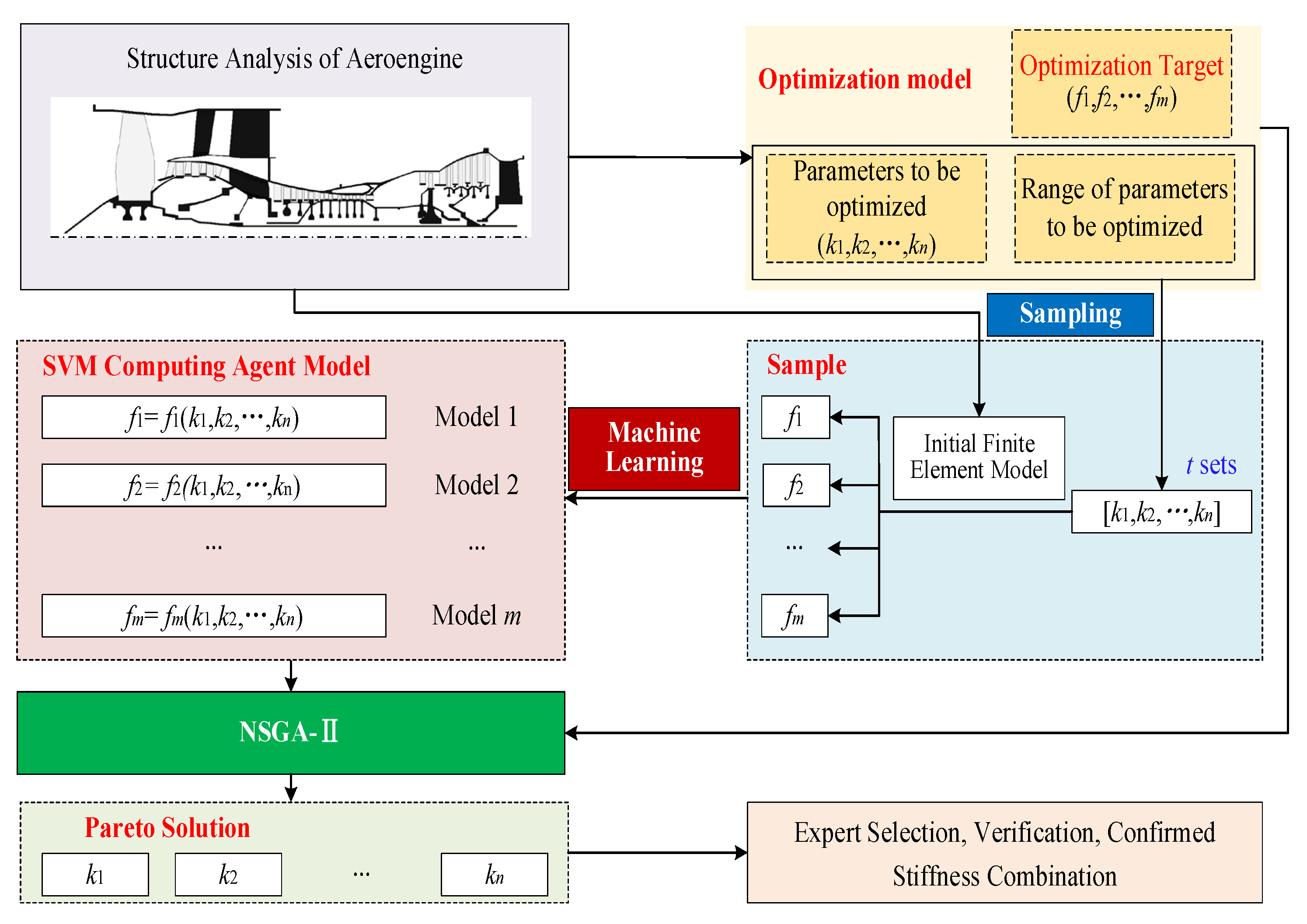
A multi-objective optimization design method for the whole aeroengine coupling vibration is proposed. The method process is shown in Figure 1, and can be divided into the following steps:

• An initial dynamic model is established, and the whole aeroengine structure is analyzed.
• The optimization model is determined, that is, the optimization objective and parameters to be optimized are determined, as well as the value range of each parameter to be optimized.
• The m sets of combined stiffness values are extracted in the n dimensional (n is the number of supports to be optimized) space with the sampling method.
• The sample points are substituted into the finite element (FE) model of the whole aeroengine as the support stiffness value and the corresponding optimization targets are calculated. Sample sets of stiffness values and optimization targets are then obtained.
• The support vector machine (SVM) computing agent model is obtained by training the sample set with the support vector regression. The explicit functional relationship between stiffness values and the optimization targets can be shown by the SVM model.
• Based on the obtained computational agent model, a set of Pareto optimal solution sets is obtained with the elitist NSGA-II.
• The obtained Pareo-optimal solution is analyzed and selected, substituted into the FE model for calculation, and the obtained result is verified, and finally the obtained optimal solution is confirmed.

2.2. Experimental Design Based on Latin Centroidal Voronoi Tessellations (LCVT)

Experimental design is a mathematical method to discretize and sample a multidimensional continuous parameter space. As it is a sampling strategy to construct an agent model, it directly affects the approximation accuracy and construction efficiency. The focus of the experimental design is to ensure that the sample points uniformly fill the whole parameter space so that the data features of the whole sample space can be fully characterized. The commonly used sampling algorithms are Latin hypercube sampling, centroidal Voronoi tessellations (CVTs), and Latin centroidal Voronoi tessellations (LCVTs).

LCVT is a sampling method that has the combined advantages of the Latin hypercube and CVT sampling methods. The fundamental idea is to first divide the high-dimensional space into n small spaces according to the number of sample points, then to take the center of gravity of each small space to form a point set, and then divide each dimension of the point set into m intervals according to the principle of equal probability. If the number of dimensions is t, the whole data space is divided into m × t cells, then a sample point is randomly selected for each cell and reassigned to that sample point. Figure 2 shows the point sets obtained by using Latin hypercube sampling, CVT sampling, and LCVT sampling methods to draw 100 sample points in the 2-dimensional space, respectively.

As shown in Figure 2, the LCVT sampling method overcomes the drawbacks of the Latin hypercube sampling method and the CVT sampling method and has improved spatial uniformity and boundary projection uniformity. In this paper, the LCVT algorithm is used to perform 4-dimensional spatial sampling of the stiffnesses of the four supports to be optimized.

2.3. Construction of Computing Agent Model Based on Support Vector Machine

The support vector machine (SVM) model is an intelligent learning method developed on the basis of statistical learning theory, which can effectively solve practical problems such as small samples, nonlinearity, and high-dimensional pattern recognition. Support vector machines are mainly divided into support vector regression (SVR) and support vector classifier. SVR are suitable for exact approximation of implicit functional relationships expressed by FE calculations. For a given training sample {(x_i, y_i), i = 1, 2,…, n}, x_i is the input vector and y_i is the desired output vector corresponding to it. SVM maps the input vector to a high-dimensional feature space using a nonlinear mapping ϕ and then performs linear regression. SVR prediction methods based on structural risk minimization theoretically guarantee the generation ability of the model under small sample learning. Therefore, with a reasonable range of values, the SVM model can accurately approximate the nonlinear function using a small training sample set. In this study, the SVR machine was used to train the sample data to obtain the regression function model of the objective function value calculated by the FE model with the stiffness value of each support.

2.4. Multi-Objective Optimization Based on NSGA-II

NSGA-II is a fast and elitist multi-objective optimization algorithm that coordinates the intermediate relationships of each objective function and satisfies the optimal values of all objective functions as much as possible. The fundamental approach is that first, the initial population is randomly generated with a population size of N, and the initial population is ranked non-dominantly. Subsequently, the initial population is selected, crossed and mutated to obtain the offspring population, then the parent population and the offspring population are combined, and then fast dominance sorting is performed on the merged population while the crowding degree of each non-dominated layer individual is calculated, and the best individual is selected to form a new parent population according to the non-dominance relationship and individual crowding degree. The new parent population is selected, crossed, and mutated to generate the next generation of child population, followed by iteration until the termination condition is satisfied. The resulting Pareto optimal solution of the system parameters is obtained.

3. Evaluation Index

3.1. Critical Speed Risk Coefficient

When an aeroengine is operated at critical speed, it will cause severe whole-engine vibration. To avoid significant damage caused by structural response, the operating speed is usually designed to be lower than the critical speed by a specific amount. The critical risk factor is defined to quantitatively measure the proximity of the critical speeds to the operating speeds. During aeroengine operation, there are m working speeds in the design speed range, W_j is the j-th working speed, and Ci is the i-th critical speed. The region j in Figure 3 is the margin region of the j-th operating speed W_j, which is the critical speed danger region of W_j. If any critical speed appears in this region, the engine will not be able to work safely with W_j. Avoid all area 1, 2,…; area m are safe areas, that is, when the critical speed appears in these areas, the aero engine can work safely at the designed working speed. In fact, the degree of danger of a certain critical speed depends on its distance from the nearest operating speed; as can be seen from Figure 3, the farther the distance, the safer the critical speed.

Thus, the critical risk factor S_i for the i-th order critical speed is defined as follows:

$$S_i=1-\underset{j=1}{\overset{m}{Min}}\left\{\frac{\left|C_i-W_j\right|}{W_j}\right\},i=1,2,\dots ,n$$

(1)

Here, C_i is the i-th critical speed; W_j is the j-th operating speed, calculate the margin of C_i for each operating speed. S_i is the difference between 1 and the minimum value of all margins. When S_i is larger, it indicates that the margin between C_i and m operating speed is smaller, that is, the closer the critical speed is to a certain working speed, the more dangerous the critical speed C_i.

3.2. Rotor Strain Energy Risk Coefficient

The rotor system is sensitive to unbalanced excitation, which can cause large vibrations under bending mode shapes, which in turn can cause failures. The greater the degree of bending, that is, the higher the proportion of the rotor bending strain energy to the strain energy of the whole engine, the more dangerous the modal shape [17]. Based on the considerations, this paper proposes the risk coefficient of rotor strain energy in order to quantitatively measure the danger degree of rotor bending mode shape under any mode shape.

The rotor strain energy risk coefficient B_i for the i-th order of modal vibration is defined as follows:

$$B_i=\frac{E_{ri}}{E_{wi}}$$

(2)

Here, 𝐸_𝑟𝑖 is the bending strain energy of the rotor in the i-th order mode shape, which can be obtained by extracting the bending strain energy of all rotor elements in the i-th order mode by the finite element software. E_wi is the total strain energy of the engine in the i-th modal order shape, including mountings, stator structures, support and rotor structures, and can be obtained by extracting the sum of the strain energy of all elements in the i-th order mode. A large B_i indicates a dangerous modal shape.

3.3. Cross-Section Rotor–Stator Rubbing Risk Coefficient

When the aero engine is operating, the stator–rotor gap value at a certain moment is equal to the closest distance between the blade tip and the inner wall of the receiver at that moment, and the direction of the static gap is the angle between the straight line and the horizontal direction composed of the two closest points. At any moment, the stator–rotor gap between the tip of each blade of the rotor of any section and the inner wall of the casing is not the same, forming a stator–rotor gap field. In actual operation, what affects the stator–rotor gap field is the displacement response of the rotor structure and the stator structure. The actual displacement response is a modal superposition, which is determined by various factors such as excitation, and is not the same at different speeds. At the critical speed, the modal mode shape of this order is excited, and the modal shape with inconsistent rotor and stator structure is easy to cause static friction, resulting in failure. In the design, it is necessary to obtain the mode shape of the rotor and stator casing from the critical speed analysis, and determine which parts are most likely to lose the gap and cause friction so as to realize the coordinated design of the mode shape of the rotor and stator structure.

To study the cross-section rotor–stator mode shape coordination and quantitatively compare the degree of the rotor–stator rubbing risk coefficient, the rotor–stator rubbing risk coefficient T_ij for cross-section j in the i-th order mode is defined as

$$T_{ij}=\frac{\left|R_{ij}-S_{ij}\right|}{\underset{j}{Max}\left|R_{ij}\right|+\underset{j}{Max}\left|S_{ij}\right|}$$

(3)

where S_ij is the static modal vibration component at section j in modal vibration mode of order i; R_ij is the rotor modal vibration component at section j in modal vibration mode of order i; $\underset{j}{Max}\left|R_{ij}\right|$ is the maximum value of rotor modal vibration component at each section of modal vibration mode of order i, and $\underset{j}{Max}\left|S_{ij}\right|$ is the maximum value of static modal vibration component at each section of modal vibration mode of order i. A large T_ij in the same order modal vibration indicates a high risk of rotor–static friction in the section.

For the three-dimensional model, take the node of each blade tip and the node modal mode shape displacement component on the stator casing corresponding to it, calculate the relative displacement of the blade tip and the casing of the whole turn, take the maximum value of the relative displacement of the rotor and the stator in the whole circle, substitute formula (3), and calculate the cross-section rotor–stator rubbing risk coefficient of this section.

4. Example of Optimizing the Support Stiffness of a Civil Turbofan Engine with a Large Bypass Ratio

4.1. Initial Finite Element Modeling and Structural Analysis

A certain dual-rotor turbofan engine with a high bypass ratio was used to establish the engine dynamics model. The engine weighed 2.80 T, had a thrown ratio of 3.80, and maximum thrust of 86.7 KN. The low-pressure rotor system consisted of 1 stage fan, 3 stage compressors, and 4 stage low-pressure turbines. The high-pressure rotor system consisted of 9 stage high-pressure compressors and 1 stage high-pressure turbine. The stator system is divided into the outer bypass casing and the inner bypass casing. The geometric model of the whole machine is established, and the semi-sectional view of the model is shown in Figure 4a, while the FE model of the whole engine is shown in Figure 4b.

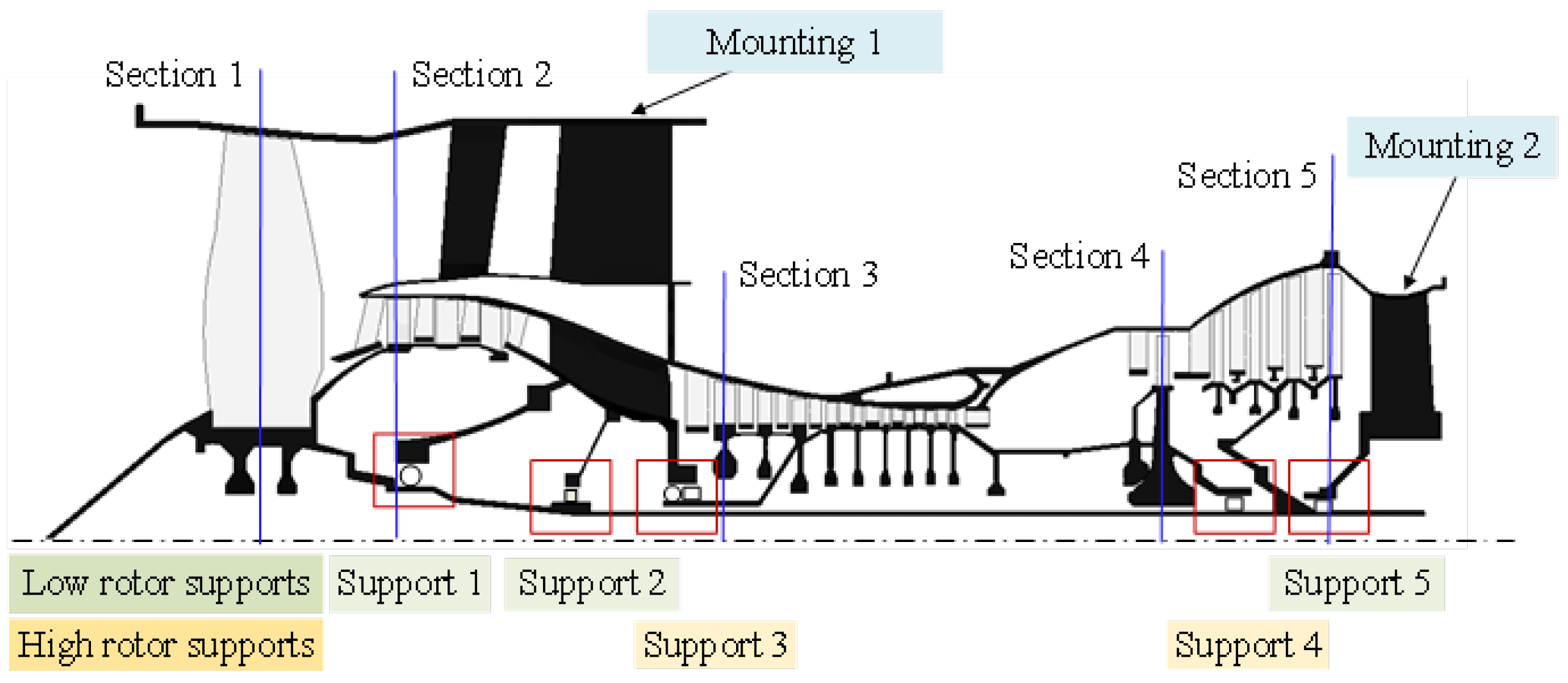
The double-rotor turbofan engine used in this study had five supports and two mountings. Its overall supports and mounting plan are shown in Figure 5. The main mounting section is located in the intermediate casing, and the auxiliary mounting section is located at the upper end of the turbine rear casing. The support stiffness value is taken as listed in

Table 1. Stiffness values of supports.

Support Number	1	2	3	4	5
Stiffness Value (107 N/m)	3.94	6.17	12	17.1	4

, and the values for the main and auxiliary mounting are set as 3 × 10⁹ N/m.

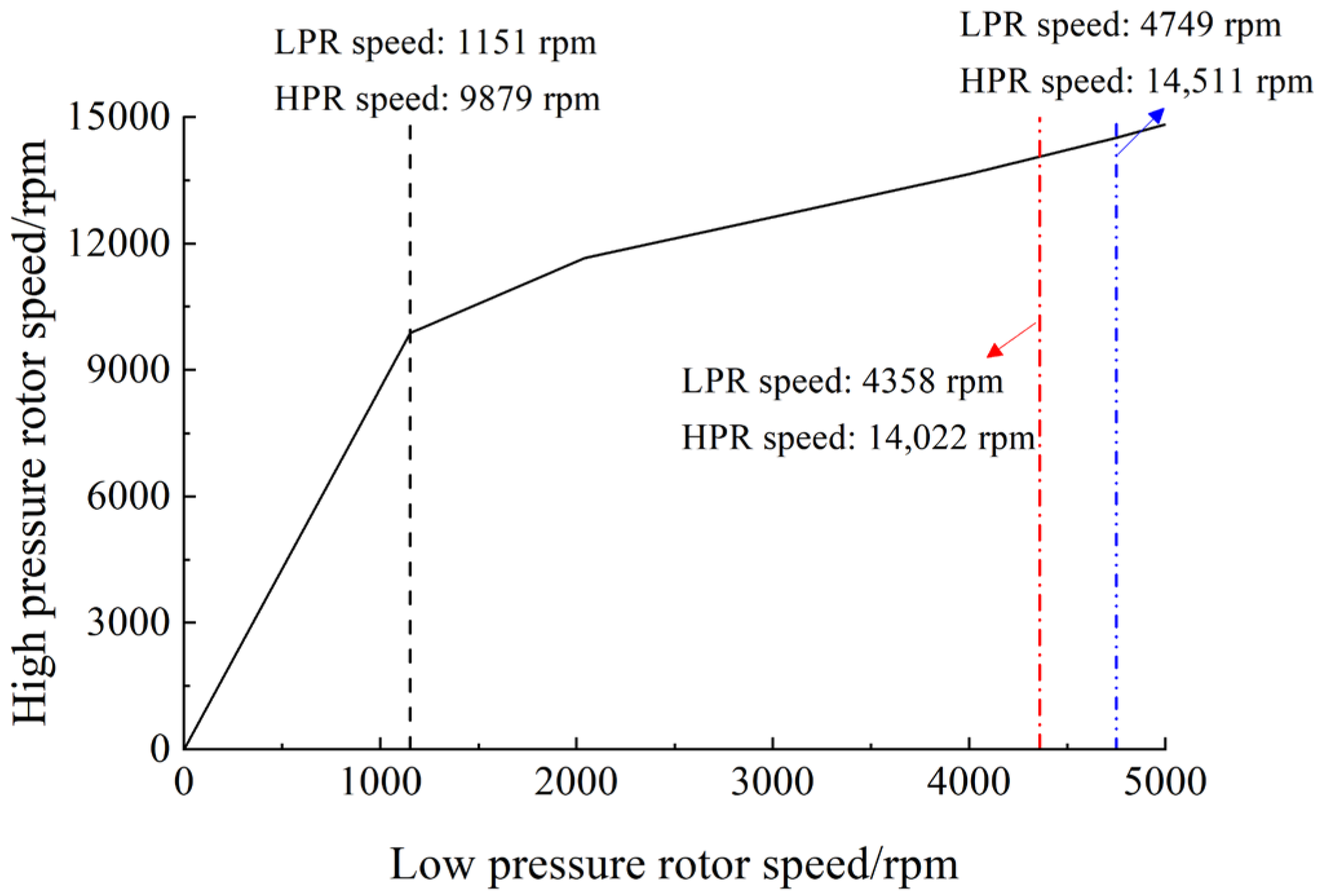
When the twin-rotor aero engine is operating, there is a certain speed relationship between the high-pressure rotor and the low-pressure rotor; usually, the method of controlling the high-pressure rotor speed and the low-pressure rotor speed adaptation is adopted to achieve speed coordination. In the whole speed range, the speed ratio of high- and low-pressure rotors is not constant, and the speed of high- and low-pressure rotors conforms to the law of common working line of high- and low-pressure rotors. The common working line of high- and low-pressure rotors of a certain type of high-bypass ratio twin-rotor aero-engine established in this paper is shown in Figure 6. In the entire speed range, there are three operating speeds, namely ground slow speed (low pressure rotor speed 1151 rpm, high-pressure rotor speed 9879 rpm), cruising speed (low-pressure rotor speed 4358 rpm, high-pressure rotor speed 14,022 rpm) and takeoff speed, that is, the maximum speed (low-pressure rotor speed 4779 rpm, high-pressure rotor speed 14,511 rpm).

Referring to the common working line of the high-pressure rotor (HPR) and low-pressure rotor (LPR) of a certain type of aero-engine, seven groups of high- and low-pressure speeds were selected on the common working line (

Table 2. High- and low-pressure rotors work together with the tachometer.

LPR speed/rpm	0	1151	2042	3000	4000	4749	5000
HPR Speed/rpm	0	9879	11,655	12,634	13,656	14,511	14,830

), and the critical speed of the system was analyzed by the Campbell diagram method.

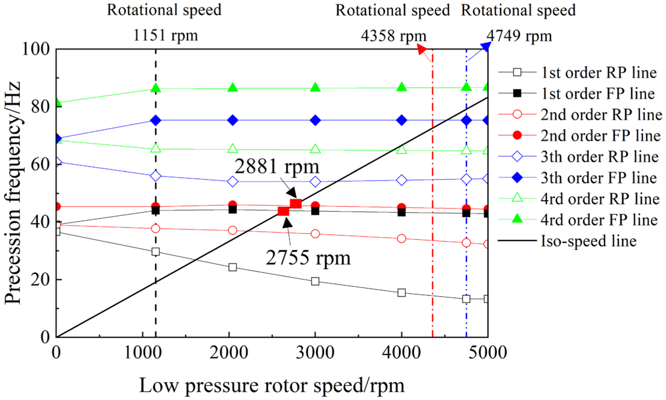
The Campbell plot is plotted with the LPR speed as the abscissa and the precession frequency as the ordinate, as shown in Figure 7. It can be seen from the figure that the critical speed of low-pressure rotor excitation in the operating speed range have two orders, 2755 rpm and 2881 rpm, respectively. Obviously, when the low-pressure rotor speed is 0 rpm, the forward and reverse precession speeds of each stage are not the same, and as the order increases, the difference between the forward and reverse precession speeds increases. This phenomenon is mainly caused by the asymmetry of rotor support stiffness in the horizontal and vertical directions.

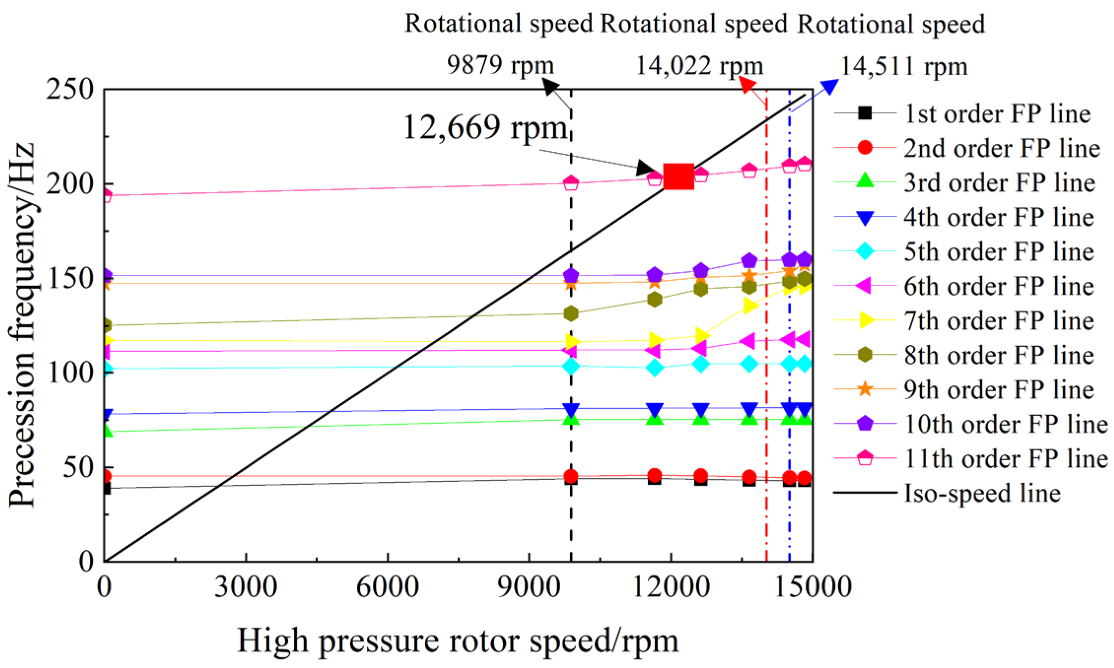
The Campbell diagram is drawn with the HPR speed as the abscissa and the precession frequency as the ordinate, as shown in Figure 8; the intersection point of the iso-speed line and the high-pressure rotor forward precession line is the critical speed of the high-pressure rotor excitation. It can be seen from the figure that the critical speed of the high-pressure rotor excitation within the operating speed range is only 1 order, which is 12,669 rpm. Due to the dense mode and clear performance, only the forward precession lines of each order are drawn for the high-pressure rotor.

The first 3 critical speed risk coefficients, rotor strain energy risk coefficients and cross-section rotor–stator rubbing risk coefficients of the engine are calculated, respectively. The structural vibration of the engine is evaluated and analyzed using three defined coefficients.

According to the calculated critical speed of the engine, the critical speed margin (that is, $\left|C_i-W_j\right|/W_j$), and then the critical speed risk coefficient of each order is obtained. Among them, the subscript L means low-pressure rotor and H means high-pressure rotor. For example, C_iL is the low-pressure rotor critical speed risk coefficient of the i-th order, and C_iH is the high-pressure rotor critical speed risk coefficient of the i-th order. W_1L represents the first operating speed of the low-pressure rotor, which is 1151 rpm, W_2L represents the second operating speed of the low-pressure rotor, which is 4358 rpm, W_3L represents the third operating speed of the low-pressure rotor, which is 4794 rpm, and W_1H, W_2H and W_3H are the corresponding the first, the second and the third high pressure rotor operating speeds, which are 9879 rpm, 14,022 rpm and 14,511 rpm respectively. The calculation process and results of the low-pressure critical speed risk coefficient and the high pressure critical speed risk coefficient of each order are shown in

Table 4. Critical speed risk coefficients of the low-pressure rotor.

Order	${\mathit{C}}_{\mathit{i}\mathit{L}}/\mathbf{rpm}$	$\left|{\mathit{C}}_{\mathit{i}\mathit{L}} - {\mathit{W}}_{\mathit{j}\mathit{L}}\right|/{\mathit{W}}_{\mathit{j}\mathit{L}}$			$\underset{\mathit{j}}{\mathit{M}\mathit{i}\mathit{n}}\left\{\frac{\left|{\mathit{C}}_{\mathit{i}\mathit{L}} - {\mathit{W}}_{\mathit{j}\mathit{L}}\right|}{{\mathit{W}}_{\mathit{j}\mathit{L}}}\right\}$	${\mathit{S}}_{\mathit{i}\mathit{L}}$
		For W1L	For W2L	For W3L
1	2755	1.394	0.368	0.420	0.368	0.632
2	2881	1.503	0.339	0.393	0.339	0.661
3	3034	1.636	0.304	0.361	0.304	0.696

and

Table 5. Critical speed risk coefficients of the high-pressure rotor.

Order	${\mathit{C}}_{\mathit{i}\mathit{H}}/\mathbf{rpm}$	$\left|{\mathit{C}}_{\mathit{i}\mathit{H}} - {\mathit{W}}_{\mathit{j}\mathit{H}}\right|/{\mathit{W}}_{\mathit{j}\mathit{H}}$			$\underset{\mathit{j}}{\mathit{M}\mathit{i}\mathit{n}}\left\{\frac{\left|{\mathit{C}}_{\mathit{i}\mathit{H}} - {\mathit{W}}_{\mathit{j}\mathit{H}}\right|}{{\mathit{W}}_{\mathit{j}\mathit{H}}}\right\}$	${\mathit{S}}_{\mathit{i}\mathit{H}}$
		For W1H	For W2H	For W3H
1	12,384	0.254	0.117	0.147	0.117	0.883
2	12,512	0.267	0.108	0.138	0.108	0.892
3	12,669	0.282	0.096	0.127	0.096	0.904

.

It can be shown in Table 4 and Table 5, the critical speed risk coefficients of the first 3 order low-pressure rotor are 0.632, 0.661 and 0.696, respectively, and the critical rotor risk coefficients of the first 3 order high-pressure rotor are 0.883, 0.892 and 0.904, respectively. Among them, the critical speed of the 3rd order high-pressure rotor is the most dangerous, and the critical speed risk coefficient reaches 0.9. Its safety should be further verified.

The strain energy analysis is carried out under the mode corresponding to each critical speed. The percentage of strain energy of each support, high- and low-pressure rotor and mountings corresponding to the three order critical speed are shown in

Table 6. Strain energy distribution at each order.

Order	${\mathit{E}}_{\mathit{w}\mathit{i}}/\mathbf{J}$	Percentage of Strain Energy/%
		${\mathit{B}}_{\mathit{i}\mathit{L}}$	${\mathit{B}}_{\mathit{i}\mathit{H}}$	Stator	Mounting 1	Mounting 2	Support 1	Support 2	Support 3	Support 4	Support 5
1	24,106	73.40	6.38	1.36	0.11	0.12	1.58	0.80	1.63	0.65	13.99
2	45,433	51.44	0.11	10.13	1.67	0.02	24.08	12.13	0.07	0.05	0.31
3	551,032	24.07	21.89	14.69	4.59	0.53	0.21	0.03	12.27	20.06	1.66

, where B_iL represents the percentage of low pressure rotor strain energy of the modal shape at the critical speed of the i-th order, which is the rotor strain energy risk coefficient of the low pressure rotor of i-th order. Similarly, B_iH represents the high-pressure rotor strain energy risk coefficient of modal shape at the i-th order critical speed.

Table 6 shows that:

1)

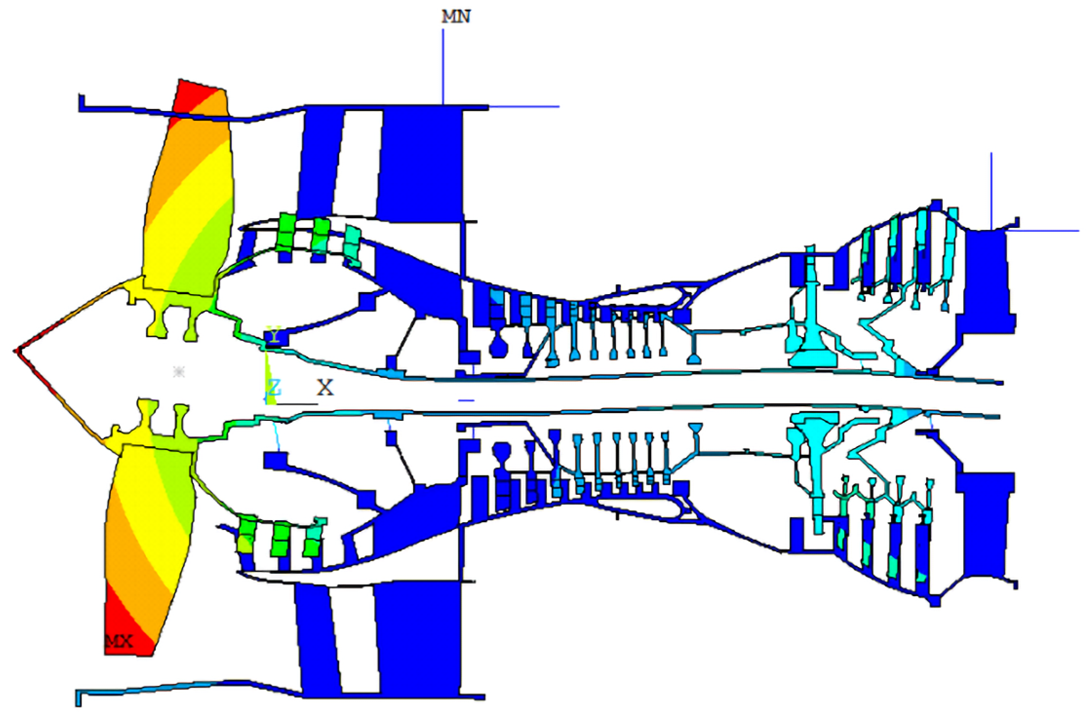
The modal shape at the 1st critical speed (N₁ = 2755 rpm, N₂ = 12,384 rpm) of low-pressure excitation is characterized by the 1st order bend of the low-pressure rotor shaft, low-pressure turbine pitch, and high-pressure rotor pitch, as shown in Figure 9. In this modal shape, 73.40% of the strain energy is concentrated on the low-pressure rotor, and this modal shape will be very sensitive to the imbalance of the low-pressure rotor, and its vibration amplitude needs to be strictly controlled. Secondly, in this modal shape, the strain energy ratio of the support 5 reaches 13.99%, which is mainly caused by the low-pressure turbine pitch of the order modal shape, and the fatigue life of the bearing should also be noted.

2)

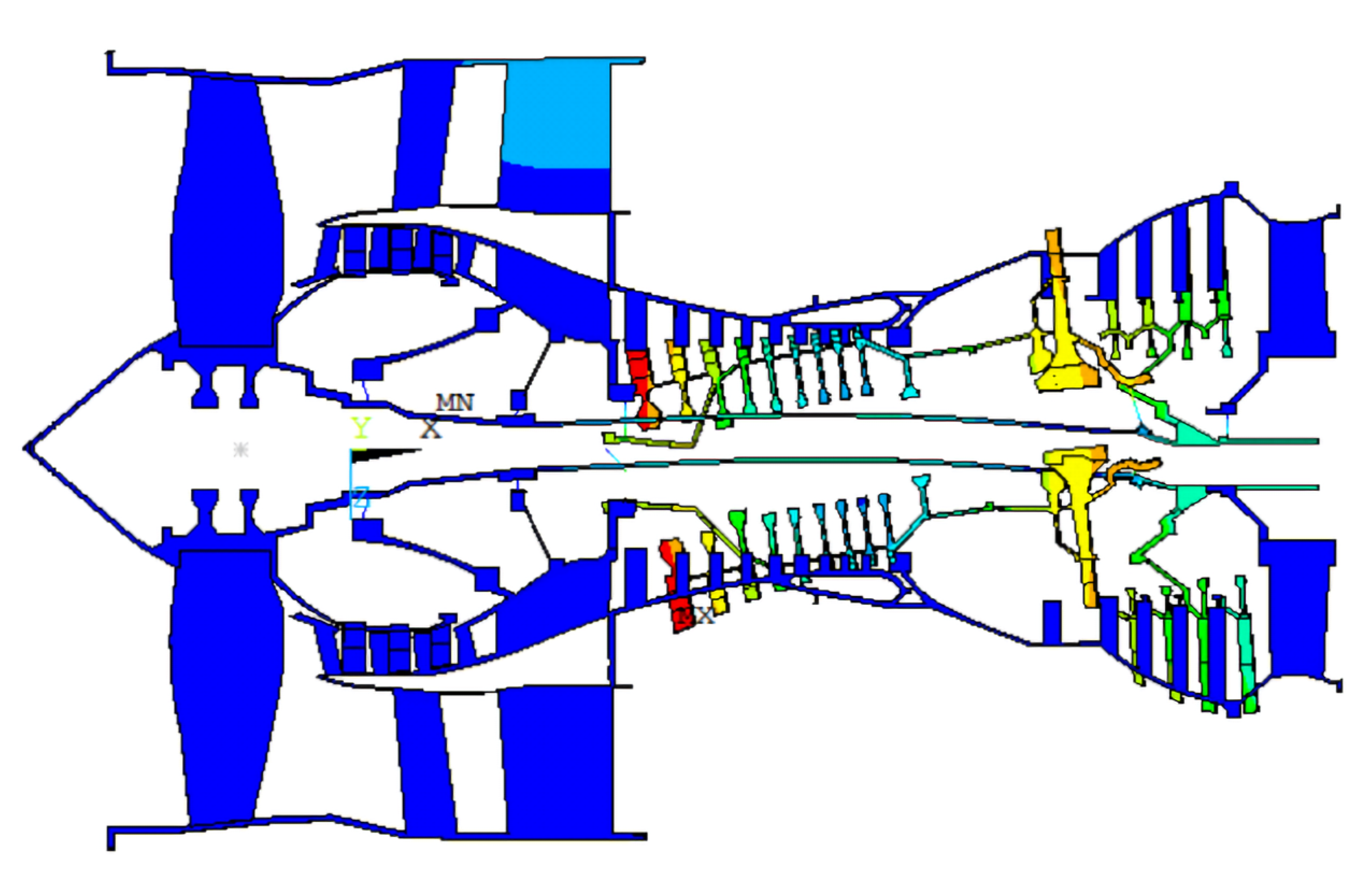
The modal shape at the 2nd critical speed (N₁ = 2881 rpm, N₂ = 12,512 rpm) excitation by low-pressure rotor is mainly manifested as fan pitch, as shown in Figure 10. 51.44% of the strain energy is concentrated in the low-pressure rotor, mainly distributed on the low-pressure fan rotor, in this order modal shape, the fan will be very sensitive to imbalance, and its dynamic balance and vibration amplitude should be strictly controlled. Support 1 withstands 24.08%, and support 2 withstands 12.13%. In this modal shape, the structural strength of the connection between the fan rotor and the low-pressure turbine rotor should attract sufficient attention. Notably, the stator withstands 10.13% of the strain energy; mainly due to support 1 and support 2, located on the stator structure, some energy transfer occurs, which alleviates the energy concentration of the low-pressure fan rotor and support 1 and support 2 to a certain extent, which is conducive to the stability of the structural vibration of the whole engine.

3)

The modal shape at the 3rd critical speed of high-pressure excitation (N₁ = 3034 rpm, N₂ = 12,669 rpm) is manifested as low-pressure rotor second-order bending, low-pressure turbine pitching, and high-pressure rotor pitching, as shown in Figure 11. In total, 24.07% of the strain energy is concentrated in the low-pressure rotor and 21.89% in the high-pressure rotor. In addition, 12.27% and 20.06% are distributed in support 3 and support 4, respectively. In this order modal shape, attention needs to be paid to the loads of support 3 and support 4. In this modal shape, the stator structure bears 14.69% of the strain energy, which is distributed in the inner and outer casing, which alleviates the load of the rotor and support to a certain extent.

According to the first three order modal shape, the five sections which have the greatest rubbing risk are selected as the key sections. Cross sections 1–5 are the fan section, the 1st stage low-pressure compressor section, the 1st stage high-pressure compressor section, high-pressure turbine section and the 4th stage low-pressure turbine section; the location of each section is shown in Figure 5. The modal displacement of the rotor tip of each key section and the corresponding stator casing position are extracted, and the modal displacement of the top node of the low-pressure rotor rectifier cone is set as 1, and each modal shape is normalized to calculate the minimum relative displacement of the rotor blade and stator casing at each section. According to Formula (3), the cross-section rotor–stator rubbing risk coefficients are calculated, as shown in

Table 7. Cross-section rotor–stator rubbing risk coefficient.

Order	$\begin{array}{l}\underset{\mathit{j}}{\overset{}{\mathit{M}\mathit{a}\mathit{x}}}\left|{\mathit{R}}_{\mathit{i}\mathit{j}}\right|+\\ \underset{\mathit{j}}{\overset{}{\mathit{M}\mathit{a}\mathit{x}}}\left|{\mathit{S}}_{\mathit{i}\mathit{j}}\right|\end{array}$	$\left|{\mathit{R}}_{\mathit{i}\mathit{j}}-{\mathit{S}}_{\mathit{i}\mathit{j}}\right|$					${\mathit{T}}_{\mathit{i}\mathit{j}}$
		Section 1	Section 2	Section 3	Section 4	Section 5	Section 1	Section 2	Section 3	Section 4	Section 5
1	59.388	0.601	0.277	0.286	2.860	1.021	0.010	0.005	0.005	0.048	0.017
2	4.805	0.653	0.366	0.025	0.097	0.072	0.136	0.076	0.005	0.021	0.015
3	221.873	8.112	6.555	27.438	20.757	17.328	0.037	0.030	0.124	0.094	0.078

.

It can be shown in Table 7:

1)

Under the 1st modal shape, the 1st order bend of the low-pressure rotor shaft, low-pressure turbine pitch, and high-pressure rotor pitch. The cross-section rotor–stator rubbing risk coefficient of Section 4 and Section 5 is large, indicating that under the modal shape, the high-pressure turbine section and the 4th stage low-pressure turbine section have a higher degree of rubbing, which is in line with the characteristics of the mode shape.

2)

Under the fan pitch modal corresponding to the 2nd order critical speed, the cross-section rotor–stator rubbing risk coefficients of Section 1 and Section 2 are the highest. It shows that under this modal shape, the fan section and the 1st stage low-pressure compressor section have a high degree of rubbing risk, which is in line with the characteristics of this modal shape.

3)

Under the 3rd modal shape, low-pressure rotor second-order bend, low-pressure turbine pitches, and high-pressure rotor pitches, Section 3 and Section 4 have the highest cross-section rotor–stator rubbing risk coefficient. It shows that under the modal shape, the 1st stage high-pressure compressor section and the high-pressure turbine section have a high degree of rubbing, which is in line with the characteristics of this modal shape.

4.2. Determining the Optimization Model

A multi-objective optimization method is used to solve the aeroengine support stiffness optimization design problem. The first three orders’ critical speed risk coefficient, rotor strain energy risk coefficient, and rotor-stator rubbing risk coefficient for five cross sections (cross section locations shown in Figure 5) are determined as the optimization objectives. Since the engine has two rotors and the three order critical speeds in the working speed range have to be analyzed, there are 27 index parameters; thus, the optimization problem becomes complicated. To solve the aeroengine support stiffness optimization problem efficiently and accurately, the calculated indicators are selected and processed. As shown in Figure 12, the most dangerous index in each group of stiffness is selected as the optimization target. The selected optimization targets are the most dangerous critical speed risk factor f₁, the highest rotor strain energy risk factor f₂ and the most dangerous rotor–stator rubbing risk coefficient f₃.

Aeroengine bearing 4 is an intermediate support. It has high stiffness and is subjected to complex working conditions including various factors, and the scope of adjustment is limited in the late design stage. Hence, it was not considered for optimization. The influence law of the stiffness of other supports on each optimization objective was analyzed. The influence laws of each support stiffness on f₁, f₂ and f₃ are shown in Figure 13, Figure 14 and Figure 15, respectively.

As shown in Figure 7, with the increase in the stiffness of support 1, f₁ first remains unchanged and then increases. The influence of support 2 on f₁ is small. Meanwhile, f₁ increases with an increase in the stiffness of support 3. With the increase in the stiffness of support 5, f₁ increases linearly.

As shown in Figure 13, with the increase in the stiffness of support 1 and support 2, f₂ decreases. Meanwhile, f₁ increases with an increase in the stiffness of support 3 and support 5.

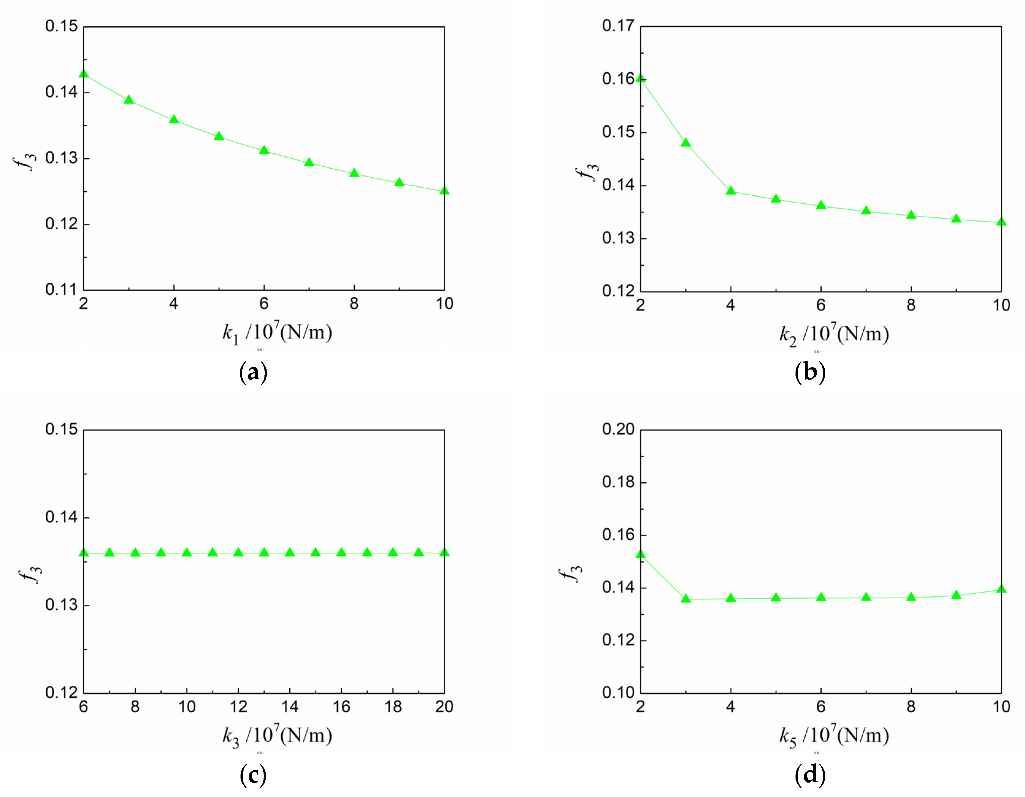
As shown in Figure 14, with the increase in the stiffness of support 1 and support 2, f₃ decreases. The influence of support 3 on f₃ is small. With the increase in the stiffness of support 5, f₃ first decreases and then remains almost unchanged.

Based on the analysis of the influence of the stiffness of each support on each optimization target, the stiffness values of supports 1, 2, 3, and 5 were determined to be the parameters to be optimized. The stiffness values of supports 1, 2, and 5 vary from 2 × 10⁷ N/m to 1 × 10⁸ N/m, and the stiffness values of support 3 range from 6 × 10⁷ N/m to 2 × 10⁸ N/m. The optimization model is finally determined as follows:

$$\left\{\begin{array}{c}\mathit{min}{f}_1\left(k_1,k_2,k_3,k_5\right)\\ \mathit{min}{f}_2\left(k_1,k_2,k_3,k_5\right)\\ \mathit{min}{f}_3\left(k_1,k_2,k_3,k_5\right)\end{array}\right.s.t.\left\{\begin{array}{c}2\times {10}^7\le k_1\le 1\times {10}^8\\ 2\times {10}^7\le k_2\le 1\times {10}^8\\ 6\times {10}^7\le k_3\le 2\times {10}^8\\ 2\times {10}^7\le k_5\le 1\times {10}^8\end{array}\right.$$

(4)

4.3. Spatial Sampling Based on LCVT

The LCVT sampling method is used to extract finite points representing all points in the space to reflect the data characteristics of the value space. In the example, after several attempts, 400 points are extracted in a 4-dimensional space. Since the 4-dimensional space cannot be visually observed, the points are plotted at 2-dimensional planes to show the sampling results. Figure 16a,b show the distribution of sampling points in the k₁-k₂ and k₁-k₃ planes, respectively.

4.4. Sample Calculation Based on Finite Element

The values of the 400 sets of k₁, k₂, k₃ and k₅ stiffness obtained by sampling are substituted into the FE model, and k₄ is taken as the original model stiffness value. The optimization target function value values under the 400 sets of sample stiffness are calculated, and a sample set consisting of k₁, k₂, k₃, k₅, and f₁, f₂, and f₃ is constructed, as shown in Figure 17. Taking f₁ as an example, for each calculation, a 5-dimensional vector consisting of k₁, k₂, k₃, k₅ and f₁ is obtained, which is a sample point. The training sample set on the objective function f₁ can be obtained by traversing all of the combinations obtained by LCVT sampling, and the training sample sets on the objective functions f₂ and f₃ can be obtained similarly.

4.5. Computing Agent Model Obtaining Based on SVM

Support vector regression analysis is performed on the obtained sample data, and the mapping relationships between f₁, f₂, f₃ and k₁, k₂, k₃ and k₅ are obtained. The mapping relationship reflects the functional relationship between the input (k₁, k₂, k₃, k₅) and the output (f₁, f₂, f₃) of the FE model, which can be shown as follows:

$$\left\{\begin{array}{c}{f}_1=f_1\left(k_1,k_2,k_3,k_5\right)\\ f_2=f_2\left(k_1,k_2,k_3,k_5\right)\\ f_3=f_3\left(k_1,k_2,k_3,k_5\right)\end{array}\right.$$

(5)

The NAGA-II parameters are set to cross probability 0.9, probability of variation 0.1, population size 1000, maximum evolutionary algebra 1000, tournament size 2, cross distribution index 20, and variation distribution index 20.

To verify the accuracy of the training model, using the cross-validation method, 350 sets of samples are selected as training samples and 50 groups of samples are selected as test samples, and three models are verified respectively; the results are shown in Figure 18. It can be used to predict the objective function values of each stiffness combination of a certain type of engine in place of the FE calculation.

As shown in the figure, the predicted objective function values are in good agreement with the actual objective function values, and the model is considered to have good generalization capability.

It can be used to predict the objective function values of each stiffness combination of a certain type of engine in place of FE calculation.

4.6. Multi-Objective Optimization Based on NSGA-II

The NSGA-II algorithm is used to solve the multi-objective optimization of the FE computing agent model established by SVM. The NSGA-II parameters are set to a crossover probability of 0.9, a mutation probability of 0.1, a population size of 1000, a maximum evolution algebra of 1000, a tournament size of 2, a cross-distribution index of 20, and a variation distribution index of 20. After 1000 iterations, the corresponding Pareto optimal solution set is obtained, as shown in Figure 19.

5. Results and Analysis

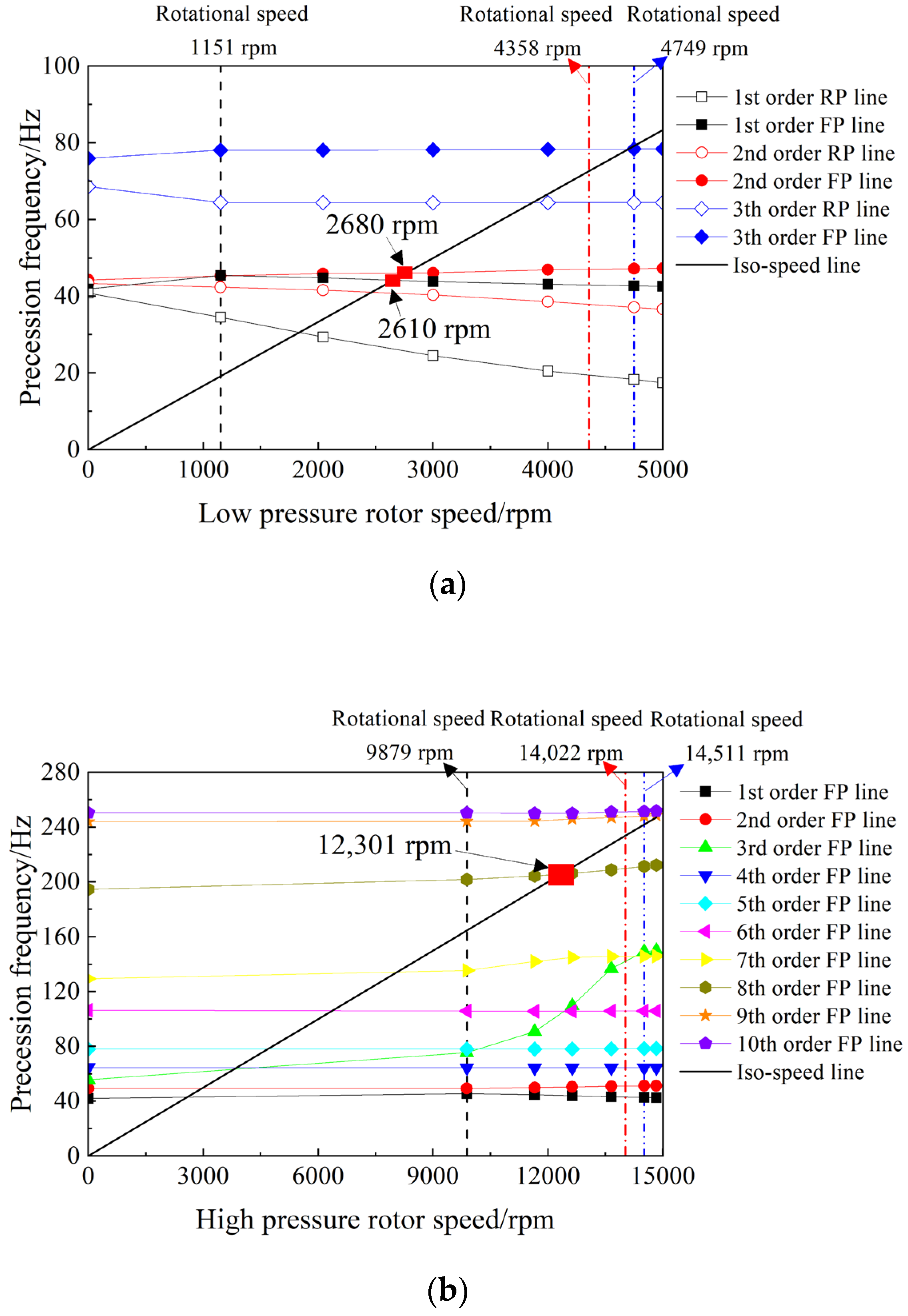
The optimal solutions of multi-objective optimization have the characteristic of mutual constraint, as a given objective cannot be optimized without degrading at least one other objective. At present, there are no unified rules for the selection of optimal solutions, and there is no absolute superiority or inferiority among the Pareto optimal solutions. The final result depends on the designer’s trade-off compromise of the objectives. The trade-off selection is made for each objective, and three sets of solutions are selected as the optimization results. The optimization results are substituted into the whole aeroengine model for FE calculation and then compared with the corresponding Pareto results. Taking group 2 as an example, the critical speed of the whole engine of the optimized model is analyzed, and the calculation method is the same as that of Section 4.1. Campbell diagrams for low-pressure rotor and high-pressure rotor excitation are calculated as Figure 20.

It can be seen from the figure that the critical speed of low-pressure rotor excitation in the operating speed range has two orders, 2610 rpm and 2680 rpm, respectively. The critical speed of the high-pressure rotor excitation within the operating speed range is only 1 order, which is 12,301 rpm. The high- and low-pressure rotor speed and modal mode shape corresponding to each critical speed are shown in

Table 8. The critical speed and mode shape of the whole engine after optimization.

Order	Critical Speed/rpm		Excitation Source	Modal Shape
	LPR	HPR
1	2610	12,235	LPR
2	2674	12,301	HPR
3	2680	12,308	LPR

LPR: low-pressure rotor; HPR: high-pressure rotor.

. Compared with

Table 3. The critical speed and mode shape of the whole engine.

Order	Critical Speed/rpm		Excitation Source	Modal Shape
	LPR	HPR
1	2755	12,384	LPR
2	2881	12,512	LPR
3	3034	12,669	HPR

LPR: low-pressure rotor; HPR: high-pressure rotor.

, it can be seen that after optimization, the critical speed of each order decreases, the order changes, and the modal mode shape of each order is basically the same as before optimization.

Refer to Section 4.1 to calculate the critical speed risk coefficient, rotor strain energy risk coefficient and section static friction risk coefficient for each step and compare them with the prediction results. The optimized support stiffness of each group is brought into the finite element model in turn, and the results are shown in

Table 9. Results of solution set selection based on the compromise of objective function.

Number	Support Value/107 (N/m)				Pareto Results			FE Calculation Results			Relative Error/%
	k1	k2	k3	k5	${\widehat{\mathit{f}}}_{\mathit{i}1}$	${\widehat{\mathit{f}}}_{\mathit{i}2}$	${\widehat{\mathit{f}}}_{\mathit{i}3}$	fi1	fi2	fi3	Δfi1	Δfi2	Δfi3
1	2.000	8.749	7.370	3.029	0.8562	0.6691	0.1257	0.8517	0.6653	0.1243	0.18	0.53	1.13
2	2.896	9.845	7.852	2.685	0.8701	0.6435	0.1259	0.8773	0.6377	0.1263	−0.82	0.91	−0.32
3	2.356	8.881	10.04	2.000	0.8634	0.6103	0.1330	0.8606	0.6074	0.1320	0.33	0.48	0.76

, where the relative error is calculated based on the FE calculation. It can be seen from Table 9 that the maximum error between the Pareto-optimal solutions and the FE calculation results of each group is only 1.13%; the results are close.

The FE calculation optimization objective values under the optimization stiffness values were compared with corresponding initial design stiffness values. The obtained result is shown in

Table 10. Optimization effect.

Number	Support Value/107 (N/m)				FE Calculation Results			Optimization Effect/%
	k1	k2	k3	k5	fi1	fi2	fi3	Δfi1	Δfi2	Δfi3
0	3.960	6.170	12.00	4.000	0.9040	0.7340	0.1360	-	-	-
1	2.000	8.749	7.370	3.0292	0.8517	0.6653	0.1243	−5.79	−9.36	−8.60
2	2.896	9.845	7.852	2.6849	0.8773	0.6377	0.1263	−2.95	−13.12	−7.13
3	2.356	8.881	10.04	2.0000	0.8606	0.6074	0.1320	−4.80	−17.25	−2.94

. The 0-th group in Table Ⅳ represents the FE calculation results obtained using the initial design stiffness values.

As shown in Table 10, the group 1 solution reduces the critical speed risk coefficient by 5.79%, the rotor strain energy risk coefficient by 9.36%, and the cross-sectional rotor-stator rubbing risk coefficient by 8.6%. The second set of solutions reduces the critical speed risk coefficient by 2.95%, the rotor strain energy risk coefficient by 13.12%, and the cross-sectional rotor-stator rubbing risk coefficient by 7.13%. The third set of solutions reduces the critical speed risk coefficient by 4.80%, the rotor strain energy by 17.25%, and the cross-sectional rotor–stator rubbing risk coefficient by 2.94%. The optimization stiffness solutions showed significant reductions in the target value characteristics compared with the original design stiffness, demonstrating the optimization of the vibration of the whole aeroengine.

6. Conclusions

In this study, a multi-objective intelligent optimization design method for whole-aeroengine coupling vibration was proposed, and the support stiffness of a turbofan engine with a large bypass ratio was optimized. Three sets of results were selected as the final optimization results. The solutions of group 1, 2, and 3 resulted in reductions in the critical speed risk coefficient of 5.79%, 2.95%, and 4.80%, respectively, reductions in the rotor strain energy risk coefficient of 9.36%, 13.12%, and 17.25%, respectively, and reductions in the cross-sectional rotor–stator rubbing risk coefficient of 8.6%, 7.13%, and 2.94%, respectively.

Risk coefficients for the critical speed, rotor strain energy, and cross-sectional rotor-stator rubbing were defined as quantitative evaluation indexes for whole-aeroengine coupled vibration, which were used as the optimization targets.

Through the optimization, multiple groups of candidate optimal solutions can be obtained, which can be selected according to the requirements in actual engineering. This study can serve as a reference for aeroengine designers. The method can also be extended to the optimization problems of other structural parameters of aeroengines.

There remain some shortcomings in this paper, for example, the evaluation system needs further improvement. This study only presents three evaluation indicators that react to the vibration of the whole machine, when the entire response problem needs consideration. In addition, there is no effective way to determine the number of samples. In future studies, this method can be extended to the optimization of other design parameters can be considered, and new sampling techniques, means of obtaining computational agent models, and multi-objective optimization methods can be used.

References

1. Cao, J.G. Research status challenge and prospect of aero-engine simulation technology. Propuls. Technol. 2018, 39, 961–970. [Google Scholar] [CrossRef]
2. Chen, Y.S.; Zhang, H.B. Review and Prospect on the Research of Dynamics of Complete Aero engine Systems. Acta Aeronaut. Astronaut. Sin. 2011, 32, 1371–1391. [Google Scholar]
3. Liu, Q.; Jiao, G. A Pipe Routing Method Considering Vibration for Aero-Engine Using Kriging Model and NSGA-II. IEEE Access 2018, 6, 6286–6292. [Google Scholar] [CrossRef]
4. Li, C.; Lei, B.; Ma, Y.H.; Hong, J. Research on Damping Vibration Reduction Design Method of Aeroengine Supporting Structure System. In Proceedings of the ASME Turbo Expo 2020: Turbomachinery Technical Conference and Exposition, Vitual, Online, 21–25 September 2020; p. V011T30A043-1-9. [Google Scholar] [CrossRef]
5. Peng, G.; Zhu, B.; Zhang, D.; Hong, J. Quantitative evaluation for the structure and mechanics properties of the high bypass ratio turbofan engines. J. Aerosol. Sci. 2017, 32, 1728–1735. [Google Scholar] [CrossRef]
6. Xu, F.Y.; Ma, H.; Zhang, L.; Hong, J. Non-deformability evaluation of aero-engine’s case. J. Aerosp. Eng. 2016, 31, 1921–1928. [Google Scholar] [CrossRef]
7. Zheng, H.Q.; Ma, Y.; Hong, J. Quantitative analysis method for mechanical characteristics of structure system in aero-engine. Chin. J. Aeronaut. 2018, 39, 645–652. [Google Scholar] [CrossRef]
8. Peng, G.; Li, C.; Zheng, H.; Ma, Y.H.; Hong, J. Quantitative Analysis Method of Whole Aero-Engine Structural Design Based on Structural Efficiency. In Mechanisms and Machine Science, Proceedings of the 10th International Conference on Rotor Dynamics–IFToMM, Rio de Janeiro, Brazil, 23–27 September; Springer: Switzerland, Cham, 2019; Volume 9, pp. 3–17. [Google Scholar] [CrossRef]
9. Copiello, D.; Ferrante, P. Multi-Objective Optimization of “True” Zero-Splice Liners for Aero-Engine Intakes. In Proceedings of the 15th AIAA/CEAS Aeroacoustics Conference, Miami, FL, USA, 11–13 May 2009. [Google Scholar] [CrossRef]
10. Chen, Y.; Cui, J.; Sun, X.; Cui, S. Research on multistage rotor assembly optimization methods for aeroengine based on the genetic algorithm. Complexity 2021, 2021, 1–14. [Google Scholar] [CrossRef]
11. Liu, J.X.; Zhang, D.Y.; Zheng, H.Q.; Hong, J. Quantitative evaluation for structure and mechanical characteristics of different thrust high bypass ratio turbo fan engines. Chin. J. Aeronaut. 2018, 39, 1077–1084. [Google Scholar] [CrossRef]
12. Zheng, L.X.; Jia, S.X.; Huang, J.J. Numerical and Experimental Study on the Multiobjective Optimization of a Two-Disk Flexible Rotor System. Int. J. Rotating Mach. 2017, 2017, 1–10. [Google Scholar] [CrossRef] [Green Version]
13. Zhang, Q.; Luo, G.H.; Fu, Y. Parameterized and optimizing design on axial flow compressor structures basing on VB Net. Mod. Mach. 2014, 2, 13–17. [Google Scholar] [CrossRef]
14. Li, L.; Yin, Z.; Qiao, W. Performance Optimal Design of Aircraft Engine Based on Multi-Objective Genetic Algorithms. J. Aerosp. Power 2006, 21, 13–18. [Google Scholar] [CrossRef]
15. Chao, L.; Fuyi, J.; Weihao, Z. Optimized design method of aero-engine rotor structure layout. J. Beijing Univ. Aeronaut. Astronautics. 2019, 45, 266–276. [Google Scholar] [CrossRef]
16. Liu, Y.Q.; Wang, D.Y.; Hong, J.; Fa, W.; Jiang, G.; Huang, H. Analysis of whole aeroengine vibration control technology. Aeroengine 2013, 39, 1–8. [Google Scholar] [CrossRef]
17. Aero-engine design manual editor-in-chief board. Aero-Engine Design Manual Volume 19: Rotordynamics and Vibration of the Whole Engine; Aviation Industry Press: Beijing, China, 2000; pp. 208–226. ISBN 7-80134-763-3. [Google Scholar]
Figure 1. Flowchart of development process for multi-objective optimization design method for aeroengine coupling vibration.
Aerospace 10 00099 g001
Figure 2. Comparison of the effect of sampling 100 sample points in two dimensions by different sampling methods. (The blue asterisk in figures are the sample points.) (a) Latin hypercube sampling; (b) CVT sampling; (c) LCVT sampling.
Aerospace 10 00099 g002
Figure 3. Schematic diagram of the relationship between critical speed and working speed.
Aerospace 10 00099 g003
Figure 4. Geometry and finite element model of a double-rotor turbofan engine with a large bypass ratio. (a) Half-sectional view of the geometry model; (b) Finite element model.
Aerospace 10 00099 g004
Figure 5. Supports and mountings of the specified engine.
Aerospace 10 00099 g005
Figure 6. High- and low-pressure rotor common working line.
Aerospace 10 00099 g006
Figure 7. Campbell diagram of low-pressure rotor excitation (FP: forward precession, RP: reverse precession).
Aerospace 10 00099 g007
Figure 8. Campbell diagram of high-pressure rotor excitation (FP: forward precession). The high- and low-pressure rotor speed and modal mode shape corresponding to each critical speed are shown in Table 3.
Aerospace 10 00099 g008
Figure 9. The first critical speed modal shape.
Aerospace 10 00099 g009
Figure 10. The second critical speed modal shape.
Aerospace 10 00099 g010
Figure 11. The third critical speed modal shape.
Aerospace 10 00099 g011
Figure 12. Optimization targets.
Aerospace 10 00099 g012
Figure 13. Effect of stiffness change of each support on f1. (a) Effect of support 1 stiffness on f1; (b) effect of stiffness of support 2 on f1; (c) effect of stiffness of support 3 on f1; (d) effect of stiffness of support 5 on f1.
Aerospace 10 00099 g013
Figure 14. Effect of stiffness change of each support on f2. (a) Effect of support 1 stiffness on f2; (b) effect of stiffness of support 2 on f2; (c) effect of stiffness of support 3 on f2; (d) effect of stiffness of support 5 on f2.
Aerospace 10 00099 g014
Figure 15. Effect of stiffness change of each support on f3. (a) Effect of support 1 stiffness on f3; (b) effect of stiffness of support 2 on f3; (c) effect of stiffness of support 3 on f3; (d) effect of stiffness of support 5 on f3.
Aerospace 10 00099 g015
Figure 16. Example of spatial distribution of LCVT sampled samples.(The blue circle in figures are the sample points.) (a) k1~k2;(b) k1~k3.
Aerospace 10 00099 g016
Figure 17. Sample calculation processes.
Aerospace 10 00099 g017
Figure 18. Model test results. (a) Model 1; (b) Model 2; (c) Model 3.
Aerospace 10 00099 g018
Figure 19. Pareto optimal solution set.
Aerospace 10 00099 g019
Figure 20. Campbell diagram after optimization. (a) Campbell diagram of low-pressure rotor excitation (FP: forward precession, RP: reverse precession); (b) Campbell diagram of high-pressure rotor excitation (FP: forward precession).
Aerospace 10 00099 g020