Variable-Geometry Rotating Components Modeling Based on Reference Characteristic Curves for the Variable Cycle Engine

Abstract

The variable cycle engine switches working modes by way of changing variable-geometry components to achieve the dual advantages of high unit thrust and low specific fuel consumption. Due to the lack of a large amount of rig test data and the complex modeling of rotating components, the incomplete characteristics of the variable-geometry rotating components lead to the non-convergence of the component-level model of the variable cycle engine, which makes it difficult to design the follow-up control system. Aiming at this problem, a characteristics modeling method of variable-geometry rotating components for variable cycle engine based on reference characteristic curves is proposed in this paper. This method establishes a neural network estimation model for the offset coefficients of key component operating points based on the characteristic law of the maturely designed variable-geometry rotating component. Combining the neural network model and the reference characteristic curves of the variable-geometry component to be designed, the offset positions of the operating points for positive and negative guide vane angles are determined. Instead of directly connecting operating points to generate characteristic lines, this paper solves the Bezier curve optimization problem based on sequential quadratic programming (SQP) to smoothly fit characteristic lines. Thereby, component characteristics that conform to the actual variable-geometry characteristics can be quickly established in the absence of rig test data. The simulations show that the characteristics of the variable-geometry rotating components established by the proposed method have satisfactory accuracy and reliability, which further improves the operation stability of the component-level model of the variable cycle engine.

1. Introduction

With the ever-expanding flight envelope and increasingly complex flight missions of aircraft, it is difficult for turbojet engines and turbofan engines with only a single working mode to meet the increasing performance requirements [1,2]. The variable cycle engine switches the working mode through the changeable geometric components so that it has the characteristics of high unit thrust and low specific fuel consumption in the corresponding flight mission, which has attracted the attention of various aviation developed countries [3]. As early as the 1960s, in order to meet the needs of multi-mission fighter jets with large flight envelope and supersonic passenger aircraft, the concept of variable cycle engines was proposed and related research was also carried out [4,5,6]. The United Kingdom designed a variable cycle engine with two shafts and three compressors, and its turbine structure was fixed. Japan has designed a variable cycle engine with variable low-pressure turbine blades [7]. France proposed a variable cycle engine scheme with an intermediate fan [8]. The United States has been a leader in variable cycle engines. GE in the United States has successively developed five generations of variable cycle engines, among which the third-generation variable cycle engine YF120 is the world’s first flight-proven variable cycle engine [9]. The primary difficulty in the application of variable cycle engines is to establish a complete and stable mathematical model for designing the subsequent control system. The difference between the variable cycle engine and the traditional aeroengine lies in the complex and changeable geometric components, including the mode selection valve, the front and rear variable aera bypass injectors, and the variable geometry rotating components [10,11]. However, the above literature does not disclose the details of modeling variable cycle engine and lacks the detailed modeling process of key geometric components [12,13,14]. This paper intends to carry out research on the modeling of variable-geometry rotating components to further increase the accuracy and reliability of variable cycle engine component-level models.

The modeling methods of rotating component characteristics are mainly divided into three categories. One is to generate performance map by aerodynamic design based on CFD [15,16]. Fang et al. continuously innovated aerodynamic design methods to design more reasonable variable area nozzle turbine (VANT) for the variable cycle engine [17,18]. Sundstrom et al. numerically explored the flow instability near surge to be more consistent with the actual fluid flow situation [19]. However, this method requires a thorough analysis of the complex fluid flow in the rotating components, which is highly difficult and time-consuming. The second modeling method is to adopt data-driven or polynomial fitting methods, etc., to generate component characteristics based on a large number of experimental data of components. Tsoutsanis et al. generated a compressor characteristic map based on elliptic function fitting of component characteristic lines [20,21,22]. Steven et al. constructed a compressor performance map based on data collected routinely from engine operation for the purpose of frequently updating and detecting shifts in the compressor performance [23]. Pau et al. predicted the pressure radio and the polytopic efficiency of a centrifugal compressor by Gaussian process regression (GPR) and support vector regression (SVR) in order for faster simulation of compressor performance than first-principle enthalpy based calculations [24]. This method requires sufficient and comprehensive data, otherwise problems such as insufficient generalization ability of component characteristics and inaccurate characteristics of some operating points are prone to occur. The last method is a combination of aerodynamic design methods and rig test data that is intended to define correction coefficients to correct the existing characteristic map so it matches the experimental data. Kurzke et al. corrected component characteristics by considering the influence of atmospheric conditions on the basis of rig test data [25,26]. Li et al. combined the genetic algorithm and the least square method to correct the characteristic map of the components based on rig test data [27]. This method is suitable for a small amount of data. However, the correction coefficients for different corrected speeds are often the same, resulting in inaccurate component characteristics.

The above-mentioned studies are basically carried out on the characteristics of the components with fixed guide vane angles, while research on the characteristics of variable-geometry components is relatively rare [28]. In component modeling, the mature variable-geometry component characteristic map is basically used directly, or the characteristic correction factor is determined based on the data of the single mode design point of the variable cycle engine and the characteristic map of fixed guide vane angles; the correction coefficients for different corrected speeds and different guide vane angles are basically the same, which makes the characteristics of the variable-geometry components inaccurate, resulting in inaccuracy and non-convergence of the component-level model when the guide vane changes [29,30]. Therefore, a method for modeling the characteristics of variable-geometry rotating components of the variable cycle engine based on the reference characteristic curves is proposed in this paper. On the one hand, when the guide vane angle becomes smaller, the change law of different components’ operating points with different corrected speeds is explored by the neural network based on the mature variable-geometry component characteristics, and the characteristics of components with positive guide vane angles are expanded by means of neural network to further increase the operating stability of the component-level model. On the other hand, based on the neural network offset coefficient estimation model and the reference characteristic curves, the offset position of the key operating points of the component characteristics to be designed is determined, and then the Bezier curve optimization problem is solved to smoothly fit the characteristic lines and obtain the more reasonable component characteristics. This method can quickly generate real and complete variable-geometry component characteristics in the absence of rig test data, which can be used for subsequent modeling and control system design.

The remainder of the paper is organized as follows: Section 2 briefly describes the establishment of the offset coefficient estimation model to determine of the offset position of the key operating points of the variable-geometry components to be designed; Section 3 mainly explores the establishment and solution of the Bezier curve optimization problem to smoothly fit the characteristic curves; in Section 4, simulation and analysis are carried out to verify the effectiveness and feasibility of the proposed method; the conclusions are summed up in Section 5.

2. Neural Network Offset Coefficient Estimation Model

Variable cycle engines have complex structures with multiple variable-geometry rotating components, the structure of which is shown in Figure 1. The numbers in the figure represent each cross section of the variable cycle engine. The number 2 represents the fan inlet, the number 21 represents the fan outlet, the number 23 represents the CDFS (core driven fan stage) inlet, the number 24 represents the CDFS outlet, the number 15 represents the first bypass, the number 3 represents the HPC (high-pressure compressor) outlet, the number 4 represents the combustion chamber outlet, the number 5 represents the LPT (low pressure turbine) outlet, the number 6 represents the internal duct outlet, the number 7 represents the nozzle inlet, the number 8 represents the nozzle throat, the number 9 represents the nozzle outlet, the number 114 represents the MSV (mode selection valve), the number 224 represents the FVABI (front-variable-area bypass injector), the number 163 represents the RVABI (rear-variable-area bypass injector). The variable cycle engine mainly includes an inlet, a fan, a CDFS, an HPC, a combustion chamber, an HPT (high pressure turbine), an LPT, a bypass, a mixer, and a nozzle. The variable-geometry components are an MSV, an FVABI, an RVABI, a CDFS with guide vane, an HPC with guide vane, and an LPT with guide vane.

This paper focuses on the CDFS to carry out related research. At present, there is the fixed guide vane angle characteristic map of the rotating components obtained from Gasturb, which is used as the reference characteristic lines for subsequent research. In addition, the corresponding angle is set as the reference angle, i.e., 0 degrees. When the guide vane angle becomes smaller than the reference angle, it is called the negative guide vane angle, and when the guide vane angle becomes larger than the reference angle, it is called the positive guide vane angle.

Most of the characteristics of the rotating components with the variable guide vane currently used are only multiplied by the correction coefficient on the basis of the fixed guide vane characteristic map, which is shown in Figure 2. The black lines in the figure are the reference characteristic lines, and the red lines are the component characteristics after the guide vane angle becomes smaller. When the guide vane angle becomes smaller, only the corrected flow rate of the same operating point becomes smaller, and the pressure ratio and efficiency remain unchanged. Obviously, this does not conform to the real situation. Figure 3 shows the characteristic map of the maturely designed CDFS (hereafter referred to as the reference characteristic map R_CDFS) in reference [29]. It can be seen from the figure that when the guide vane angle becomes smaller, not only does the corrected flow rate become smaller, but the pressure ratio and efficiency also become smaller. Therefore, the neural network is used to learn the deviation law of the component operating points when the guide vane angle changes in the R_CDFS and to establish the offset coefficient model. Based on the offset coefficient model, the deviation law can be transferred to the characteristics map of the CDFS to be designed (hereafter referred to as D_CDFS).

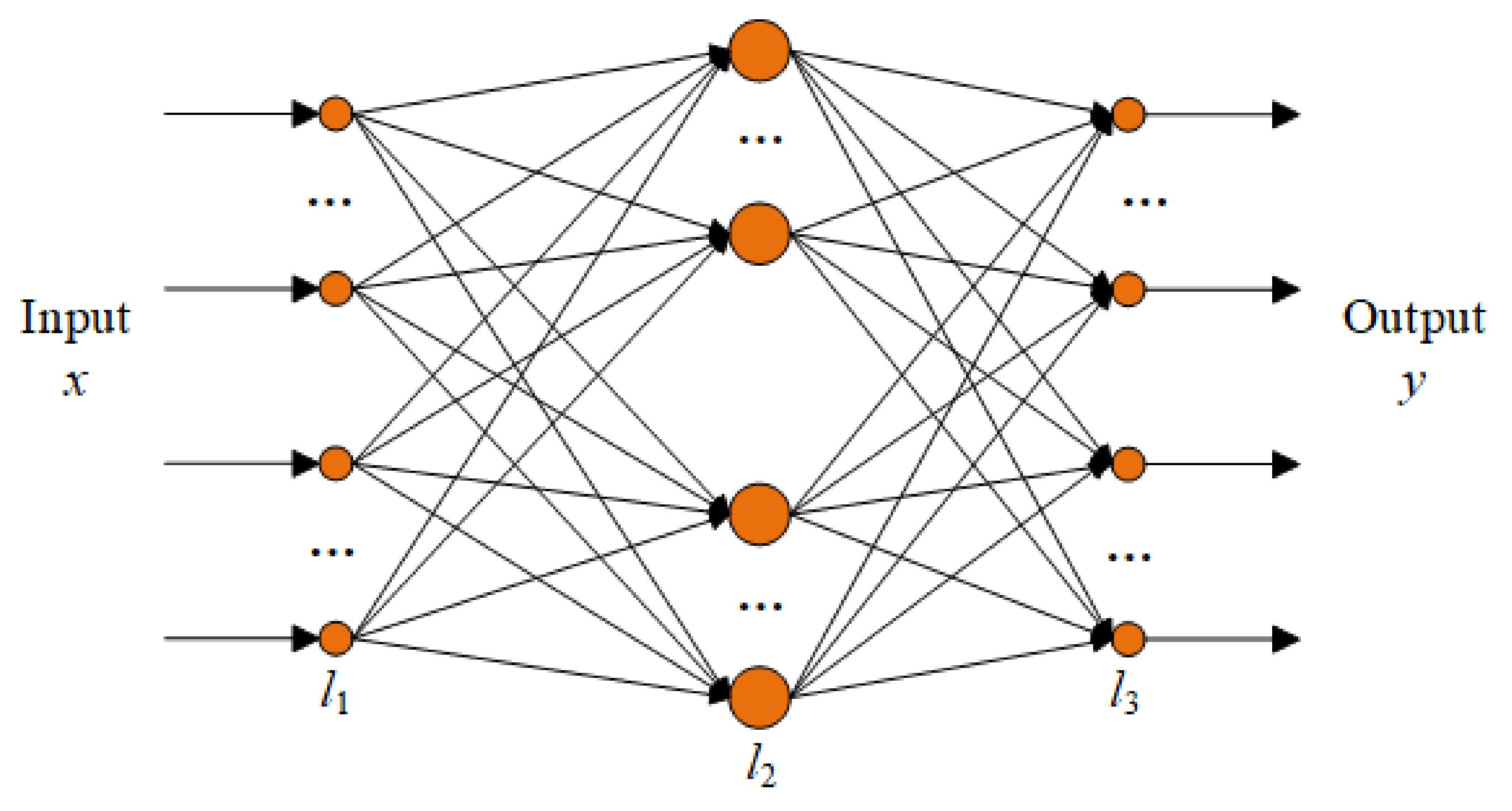
2.1. BP Neural Network

BP neural network is adopted to establish the offset coefficient estimation model, and the topology structure is shown in Figure 4. In the figure, $N_{\mathrm{i}}(i=1,2,3)$ is the number of nodes of the ith layer, $w_{nj}^{(i)}$ is the connection weight between neuron $n$ of the ith layer, and neuron $j$ of the (i − 1)th layer. x is the input of the neural network, and y is the output of the neural network.

The mapping relationship of the neural network is as follows:

$$\mathit{y}=f(\mathit{x}).$$

(1)

The specific training process is as follows. Suppose S training samples are used to train the network, one of which is sample s. For sample s, the input of the nth neuron of the ith layer is as follows:

$$ne{t}_{ns}^{(i)}=\{\begin{array}{c}{x}_n i=1\\ {\displaystyle \sum _{j=1}^{N_{i-1}}{w}_{nj}^{(i)}{o}_{js}^{(i-1)}}-{\theta }_n^{(i)} i=2,3\end{array} ,$$

(2)

where ${\theta }_n^{(i)}$ is the threshold of the neuron n of the ith layer, $o_{js}^{(i-1)}$ is the output of neuron j of the (i − 1)th layer of sample s.

The output of the nth neuron of the ith layer is as follows:

$$o_{ns}^{(i)}=\{\begin{array}{c}ne{t}_{ns}^{(i)} i=1\\ g(ne{t}_{ns}^{(i)}) i=2,3\end{array} ,$$

(3)

where $g(\cdot )$ is the activation function.

The loss function for S training samples is as follows:

$$L=\frac{1}{2}{\displaystyle \sum _{s=1}^S{\displaystyle \sum _{n=1}^{N_3}{\left(t_{ns}-y_{ns}\right)}^2}}=\frac{1}{2}{\displaystyle \sum _{s=1}^S{\displaystyle \sum _{n=1}^{N_3}{\left(t_{ns}-o_{ns}^{(3)}\right)}^2}} ,$$

(4)

where $y_{ns}$ is the output of the output node n of sample s, and $t_{ns}$ is the target output of the output node n of sample s.

If the learning process adjusts the weighting coefficient in the direction where L decreases the fastest, then the weighting coefficient of any neuron n in the ith layer is as follows:

$$\{\begin{array}{c}{w}_{nj}^{(i)}\left(k+1\right)=w_{nj}^{(i)}\left(k\right)+\eta {\displaystyle \sum _{s=1}^S{\delta }_n^{(i)}{o}_{js}^{(i-1)}} i=2,3\\ {\delta }_n^{(i)}=\{\begin{array}{c}{o}_{ns}^{\left(i\right)}(1-o_{ns}^{\left(i\right)})(t_{ns}-o_{ns}^{\left(i\right)}) i=3\\ o_{ns}^{\left(i\right)}(1-o_{ns}^{\left(i\right)})\left[{\displaystyle \sum _{n=1}^{N_{i+1}}{\delta }_n^{(i+1)}{w}_{nj}^{(i+1)}(k+1)}\right] i=2\end{array}\end{array} ,$$

(5)

where $\eta$ is the learning efficiency, $\eta$ > 0. The training process of BP neural network is to constantly adjust the weighting coefficient until the loss function meets the requirements.

2.2. Training and Testing of Neural Network Offset Coefficient Estimation Model

After determining the topology of the neural network, it is necessary to determine the training data of the neural network. Each corrected speed line of the reference characteristic lines has multiple component operating points, and due to the lack of more detailed data, it is difficult to determine the specific position of the component operating points on the characteristic lines when the guide vane angle is changed. Only the positions of three operating points can be determined on each corrected speed characteristic line. Taking the maximum speed line of the reference lines in R_CDFS as an example, the three points taken on this characteristic line are shown in Figure 5. So, the three operating points of the surge boundary point o₁, the peak efficiency point o₂, and the stall boundary point o₃ are selected as reference objects. We calculate the offset coefficient of the corrected flow rate $k_w$, the offset coefficient of the pressure ratio $k_{\pi }$, and the offset coefficient of the efficiency $k_{\eta }$ of these three operating points on each corrected speed line in the reference characteristic lines when the guide vane angle changes, as shown in Equation (6):

$$\{\begin{array}{l}{k}_w(\Delta \alpha ,n_{cor},o_i)=w_{\alpha ,R_{\mathrm{CDFS}}}(\Delta \alpha ,n_{cor},o_i)/w_{0,R_{\mathrm{CDFS}}} (0,n_{cor},o_i) i=1,2,3\\ k_{\pi }(\Delta \alpha ,n_{cor},o_i)={\pi }_{\alpha ,R_{\mathrm{CDFS}}}(\Delta \alpha ,n_{cor},o_i)/{\pi }_{0,R_{\mathrm{CDFS}}} (0,n_{cor},o_i) i=1,2,3\\ k_{\eta }(\Delta \alpha ,n_{cor},o_i)={\eta }_{\alpha ,R_{\mathrm{CDFS}}}(\Delta \alpha ,n_{cor},o_i)/{\eta }_{0,R_{\mathrm{CDFS}}} (0,n_{cor},o_i) i=1,2,3\end{array} ,$$

(6)

where $\Delta \alpha$ is the variation of the guide vane angle, $n_{cor}$ is the corrected speed, $o_i(i=1,2,3)$ are the different operating points, $w$ is the corrected flow rate of the operating point, $\pi$ is the pressure ratio of the operating point, $\eta$ is the efficiency of the operating point, subscript 0 represents the guide vane angle of the reference characteristic lines, the subscript $\alpha$ represents the change of $\Delta \alpha$ in the reference guide vane angle, and the subscript R_CDFS represents the characteristic map of the maturely designed CDFS.

Since only three operating points are selected for each characteristic line, the number of training samples is too small, so multiple speed characteristic lines are obtained by two-dimensional interpolation to expand the training samples, as shown in Figure 6. In the figure, the characteristic map with guide vane angle of 0 is taken as an example to show the characteristic map after the expansion of two-dimensional interpolation.

We calculate the operating points’ offset coefficient of each corrected speed reference characteristic line in R_CDFS when the guide vane angle changes. The offset coefficients of key operating points on the characteristic line whose corrected speed is equal to 0.7 are taken as test samples, and the rest data are taken as training samples for BP neural network training. The neural network topology has been described in Section 2.1. The number of hidden layers in the neural network is set to 1 and the number of hidden layer nodes is set to 50. The mapping relationship is shown in Equation (7):

$$\begin{array}{c}\mathit{y}=f\left(\mathit{x}\right)\hfill \\ \mathit{x}=[n_{c\alpha },\Delta \alpha ,s]{}^{\mathrm{T}}\hfill \\ \mathit{y}=[k_w,k_{\pi },k_{\eta }]{}^{\mathrm{T}},\hfill \end{array}$$

(7)

where x is the input of the neural network, and y is the output of the neural network. $s(s=1,2,3)$ is the label of the corresponding operating point $o_{\mathrm{i}}(\mathrm{i}=1,2,3)$.

After training the neural network offset coefficient estimation model, the test samples are used for testing, and the test results are shown in

Table 1. Test error of neural network offset coefficient estimation model.

	$k_w$	$k_{\pi }$	$k_{\eta }$
RMSE	0.39%	0.36%	0.35%

. It can be seen from the table that the RMSE of each offset coefficient is less than 0.5%, and the neural network offset coefficient estimation model established in this paper has a relatively high precision.

According to the trained offset coefficient estimation model, the relationship between the offset coefficients $k_w$, $k_{\pi }$, $k_{\eta }$, the corrected speed, and the change in the guide vane angle can be obtained as shown in Figure 7. It can be seen from the figure that the offset coefficient has a basically monotonic relationship with the corrected speed and the variation of the guide vane angle.

3. Generation of Characteristic Maps Based on Bezier Curve Optimization

Based on the trained offset coefficient estimation model and the reference characteristic lines in D_CDFS, the offset positions of the key operating points on the reference characteristic lines when the guide vane angle changes can be obtained, as shown in Equation (8). In this way, the characteristics of variable-geometry rotating components in R_CDFS can be quickly and accurately transferred to the characteristic map of CDFS to be designed, i.e., D_CDFS.

$$\{\begin{array}{l}{w}_{\alpha ,D_{CDFS}}(\Delta \alpha ,n_{cor},o_i)=k_w(\Delta \alpha ,n_{cor},o_i)\cdot w_{0,D_{CDFS}}(0,n_{cor},o_i) i=1,2,3 \\ {\pi }_{\alpha ,D_{CDFS}}(\Delta \alpha ,n_{cor},o_i)=k_{\pi }(\Delta \alpha ,n_{cor},o_i)\cdot {\pi }_{0,D_{CDFS}} (0,n_{cor},o_i) i=1,2,3 \\ {\eta }_{\alpha ,D_{CDFS}}(\Delta \alpha ,n_{cor},o_i)=k_{\eta }(\Delta \alpha ,n_{cor},o_i)\cdot {\eta }_{0,D_{CDFS}} (0,n_{cor},o_i) i=1,2,3 \end{array}.$$

(8)

So far, three operating points on the characteristic line of constant corrected speed under different guide vane angles in D_CDFS have been determined. Each characteristic line is not a strict quadratic curve, so it is difficult to obtain a smooth characteristic line only by polynomial fitting. Therefore, this paper establishes an optimization problem based on the Bezier curve to smoothly fit the characteristic line and generate a complete characteristic map.

3.1. Bezier Curve

The good controllability of Bezier curve makes it widely used in engineering [31,32]. For n+1 control points $P_i(i=0,1,\dots ,n)$ in a given space, Bezier curve can be defined as

$$P(t)={\displaystyle \sum _{i=0}^n{P}_i{B}_{i,n}(t),t\in [0,1]},$$

(9)

where $B_{i,n}(t)$ is a Bernstein basis function of degree n.

$$B_{i,n}(t)=C_n^i{t}^i{(1-t)}^{n-i},C_n^i=\frac{n!}{(n-1)!i!},(i=0,1,\dots n),$$

(10)

where $0^0=1,0!=1$. The sum of Bernstein basis functions is 1,

$${\displaystyle \sum _{i=0}^n{B}_{i,n}(t)}={\displaystyle \sum _{i=0}^n{C}_n^i{t}^i{(1-t)}^{n-i}}={(t+1-t)}^n=1.$$

(11)

Figure 8 shows the Bezier curve of order 3, in which P₀, P₁, P₂ and P₃ are the control points of Bezier curve, $P_0^{\prime },P_1^{\prime },P_2^{\prime },P_0^{″},P_1^{″},P_0^{\prime ″}$ are the newly determined control points on the corresponding lines by changing the value of t, and the final control point is the point on Bezier curve.

$$t=\frac{P_{start}{P}^{\prime }}{P_{start}{P}_{end}}=\frac{P_0{P}_0^{\prime }}{P_0{P}_1}=\frac{P_1{P}_1^{\prime }}{P_1{P}_2}=\frac{P_2{P}_2^{\prime }}{P_2{P}_3}=\frac{P_0^{\prime }{P}_0^{″}}{P_0^{\prime }{P}_1^{\prime }}=\frac{P_1^{\prime }{P}_1^{″}}{P_1^{\prime }{P}_2^{\prime }}=\frac{P_0^{″}{P}_0^{\prime ″}}{P_0^{″}{P}_1^{″}}.$$

(12)

Because Bezier curve is the weighted sum of Bernstein basic functions and control points, and the sum of all Bernstein basic functions is 1, Bezier curve is within the convex hull surrounded by control points, as shown by the shaded area in the figure, and the convex hull makes it possible to control the curve well when designing Bezier curve. The Bezier curve is controlled by controlling the range of control points. In this paper, Bezier curves are designed for each characteristic line based on three obtained operating points to obtain a complete and smooth characteristic line.

3.2. Construction of Bezier Curve Optimization Problem

According to Section 2.2, the three key operating points are the surge boundary point o₁, the peak efficiency point o₂ and the stall boundary point o₃. It is difficult to approximate the trend of a characteristic line with a Bezier curve. Therefore, the connecting line between o₁ and o₂ is defined as l₁, and the connecting line between o₂ and o₃ is defined as l₂. For these two lines, Bezier curve optimization problems are established, respectively.

Firstly, the characteristic map of efficiency and corrected flow rate is studied. l₁ and l₂ are approximated by third-order Bezier curves, so each line needs to determine four control points, namely P₀, P₁, P₂, P₃. Because the efficiency and the corrected flow rate of three operating points are known, i.e., the starting point and ending point of each line are determined, each line needs to determine the remaining two control points, namely, $P_1^{l_1},P_2^{l_1},P_1^{l_2},P_2^{l_2}$, to optimize the Bezier curve. Taking the efficiency, the corrected flow rate of the starting point, and the corrected flow rate at the ending point as known variables, the efficiency and corrected flow rate of the remaining points and the efficiency of the ending point are regarded as the variables to be optimized, that is as follows:

$${\mathrm{u}}_{\eta }={[w_{p_1,l_1},w_{p_2,l_1},w_{p_1,l_2},w_{p_2,l_2},{\eta }_{p_1,l_1},{\eta }_{p_2,l_1},{\eta }_{p_3,l_1},{\eta }_{p_1,l_2},{\eta }_{p_2,l_2},{\eta }_{p_3,l_2}]}^{\mathrm{T}}.$$

(13)

The optimization objective is as follows:

$$J_{\eta }=q_{\eta }\ast {({\eta }_{P_3,l_1}-{\eta }_{o_2})}^2+r_{\eta }\ast {({\eta }_{P_3,l_2}-{\eta }_{o_3})}^2 q_{\eta },r_{\eta }\in [0,1],$$

(14)

where $q_{\eta }$ and $r_{\eta }$ are weight coefficients, ${\eta }_{P_3,l_1}$ represents the efficiency of the fourth control point P₃ on line l₁, ${\eta }_{o_2}$ represents the efficiency of the ending point on l₁, namely, the peak efficiency point o₂, ${\eta }_{P_3,l_2}$ represents the efficiency of the fourth control point P₃ on line l₂, and ${\eta }_{o_3}$ represents the efficiency of the ending point on l₂, namely, the stall boundary point o₃.

Based on the variables to be optimized, two lines, l₁ and l₂, can be generated. Assuming that there are ten points on each line, the efficiency and the corrected flow rate of these points needs to meet the following constraints:

$$\{\begin{array}{l}{w}_{i,l_1}<w_{i+1,l_1},i=1,2,\dots 9\\ w_{i,l_2}<w_{i+1,l_2},i=1,2,\dots 9\\ \{\begin{array}{l}if {\eta }_{o_1}<{\eta }_{o_2},{\eta }_{i,l_1}<{\eta }_{i+1,l_1},i=1,2,\dots 9\\ if {\eta }_{o_1}>{\eta }_{o_2},{\eta }_{i,l_1}>{\eta }_{i+1,l_1},i=1,2,\dots 9\end{array}\\ {\eta }_{i,l_2}>{\eta }_{i+1,l_2},i=1,2,\dots 9\\ \{\begin{array}{l}if {\eta }_{o_1}<{\eta }_{o_2},({\eta }_{i+2,l_1}-{\eta }_{i+1,l_1})\le ({\eta }_{i+1,l_1}-{\eta }_{i,l_1}),i=1,2,\dots 8\\ if {\eta }_{o_1}>{\eta }_{o_2},({\eta }_{i+2,l_1}-{\eta }_{i+1,l_1})\ge ({\eta }_{i+1,l_1}-{\eta }_{i,l_1}),i=1,2,\dots 8\end{array}\\ ({\eta }_{i+2,l_2}-{\eta }_{i+1,l_2})\ge ({\eta }_{i+1,l_2}-{\eta }_{i,l_2}),i=1,2,\dots 8\end{array} .$$

(15)

The first five inequalities of the constraints are to reflect that, with the increase of corrected flow rate, if the efficiency of the surge boundary point is less than that of the peak efficiency point, the efficiency will first increase and then decrease; otherwise, the efficiency will decrease monotonously. The last three inequalities reflect the trend of the change rate of efficiency.

For the characteristic map of pressure ratio and corrected flow rate, two third-order Bezier curves are still used to approximate l₁ and l₂. Because of the optimization of the characteristic map of efficiency and corrected flow rate, the corrected flow rate of each control point has been determined. Therefore, the variables to be optimized in this characteristic map are as follows:

$${\mathit{u}}_{\pi }={[{\pi }_{p_1,l_1},{\pi }_{p_2,l_1},{\pi }_{p_3,l_1},{\pi }_{p_1,l_2},{\pi }_{p_2,l_2},{\pi }_{p_3,l_2}]}^{\mathrm{T}}.$$

(16)

The optimization objective is as follows:

$$J_{\pi }=q_{\pi }\ast {({\pi }_{P_3,l_1}-{\pi }_{o_2})}^2+r_{\pi }\ast {({\pi }_{P_3,l_2}-{\pi }_{o_3})}^2 q_{\pi },r_{\pi }\in [0,1],$$

(17)

where $q_{\pi }$ and $r_{\pi }$ are weight coefficients, ${\pi }_{P_3,l_1}$ represents the pressure ratio of the fourth control point P₃ on line l₁, ${\pi }_{o_2}$ represents the pressure ratio of the ending point on l₁, namely, the peak efficiency point o₂, ${\pi }_{P_3,l_2}$ represents the pressure ratio of the fourth control point P₃ on line l₂, and ${\pi }_{o_3}$ represents the pressure ratio of the ending point on l₂, namely, the stall boundary point o₃.

Similarly, based on the variables to be optimized, two lines, l₁ and l₂, can be generated. Assuming that there are ten points on each line, the pressure ratio and the corrected flow rate of these points needs to meet the following constraints:

$$\{\begin{array}{l}{\pi }_{i,l_1}>{\pi }_{i+1,l_1},i=1,2,\dots 9\\ {\pi }_{i,l_2}>{\pi }_{i+1,l_2},i=1,2,\dots 9\\ ({\pi }_{i+2,l_1}-{\pi }_{i+1,l_1})\ge ({\pi }_{i+1,l_1}-{\pi }_{i,l_1}),i=1,2,\dots 8\\ ({\pi }_{i+2,l_2}-{\pi }_{i+1,l_2})\ge ({\pi }_{i+1,l_2}-{\pi }_{i,l_2}),i=1,2,\dots 8\\ ({\pi }_{2,l_2}-{\pi }_{1,l_2})\ge ({\pi }_{10,l_1}-{\pi }_{9,l_1})\end{array} .$$

(18)

These constraints reflect that the pressure ratio decreases monotonously, and the change rate of pressure ratio increases monotonously with the increase of corrected flow rate in the characteristic map of the pressure ratio and corrected flow rate.

3.3. Method Verification

In this paper, SQP algorithm is used to solve the above optimization problems. Take the reference characteristic lines in D_CDFS as an example for verification, as shown in Figure 9. It can be seen from the figure that the characteristic map generated by Bezier curve optimization basically coincides with the original characteristic map, and the error between them is small, which is obviously better than the characteristic map formed by directly connecting three operating points. The method of fitting characteristic lines designed in this paper is certain effective and feasible.

The method designed in this paper is applied to fit the characteristic line under other guide vane angles, and the final characteristic map of CDFS with variable-geometry is shown in Figure 10. In order to further expand the working range of variable-geometry components and improve the stability of the component-level model of the variable cycle engine, this paper also expands the characteristic map under positive guide vane angle based on the above-mentioned offset coefficient estimation model and Bezier curve optimization method; that is, the characteristic map under the guide vane angle of 15 degrees in the figure.

4. Simulation and Analysis

Taking the variable cycle engine with the single bypass mode as an example, the generated characteristics of guide vane angle with positive and negative opening degree are applied to the component-level model of the variable cycle engine to analyze the performance of CDFS. Given the control variables and state variables, only the fuel flow rate is changed to simulate the acceleration process of the variable cycle engine, and the change curve of the fuel flow rate is shown in Figure 11. The fuel flow rate value in the figure have been normalized based on the fuel flow rate value of the design point of the variable cycle engine with single bypass mode.

During the acceleration process of the variable cycle engine, the position change curve of the component’s operating point on the characteristic map with the change of the guide vane angle is obtained, as shown in Figure 12. As can be seen from the figure, under the condition of the same control variables, when the guide vane angle increases, the flow rate of the operating point increases, the pressure ratio increases, and the efficiency increases. The surge margin (SM) of CDFS becomes smaller, and it is easy to surge, which reduces the operation safety of the component, as shown in Figure 13.

The reason may be that when the guide vane angle becomes smaller, the flow area of airflow becomes smaller, as shown in Figure 14. Therefore, the flow rate becomes smaller and the efficiency decreases. When the fuel flow rate is constant, the speed of the variable cycle engine decreases, the power of CDFS decreases so the pressure ratio decreases, and the operating point of the component is far away from the surge boundary point so the surge margin increases, and the operation stability of components increases.

Therefore, the characteristic modeling method for the variable-geometry component of the variable cycle engine based on the reference characteristic line can reflect the characteristics of variable-geometry components. During the operation of the engine, through adjusting the guide vane angle of the variable-geometry component, the surge margin of the component can be effectively adjusted while ensuring the engine performance.

5. Conclusions

A modeling method based on reference characteristic curves for variable-geometry rotating components of the variable cycle engine is proposed in this paper. The following conclusions can be drawn:

• BP neural network is adopted to learn the deviation law of operating points in the maturely designed characteristics, which is transferred to the characteristics to be designed so as to generate the desired characteristics quickly and accurately in the absence of rig test data. Simulations show that the offset coefficient estimation model based on the BP neural network has a certain accuracy, and compared with the existing method of modifying the variable-geometry components’ characteristics by the same correction factor, this method is more in line with the actual characteristics;
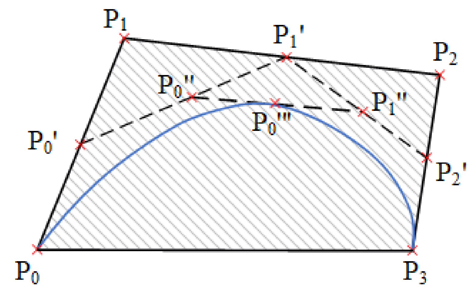
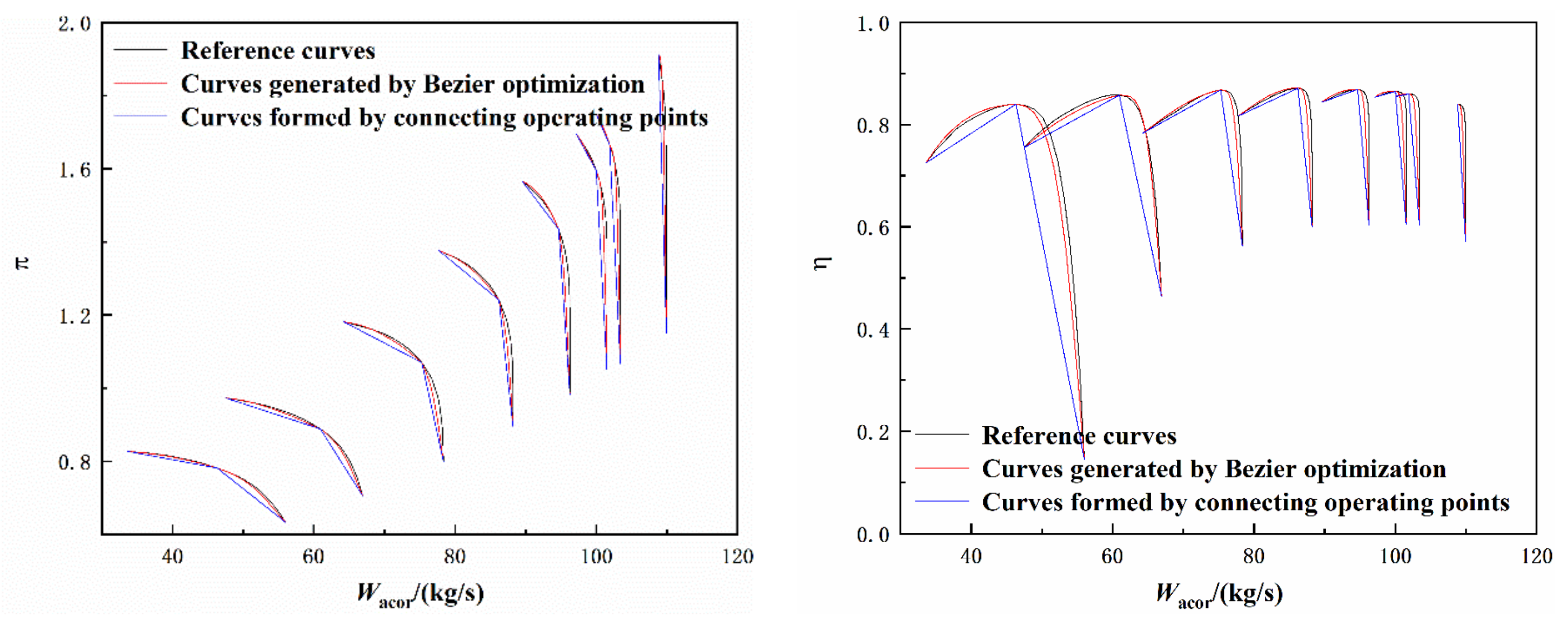
• The method proposed in this paper is to establish the Bezier curve optimization problem and solve it with SQP to smooth fit characteristic lines. The simulations show that the characteristic line generated by this method is better than that generated by directly connecting the operating points of components, and the error between the generated characteristic lines and the real characteristic lines is small;
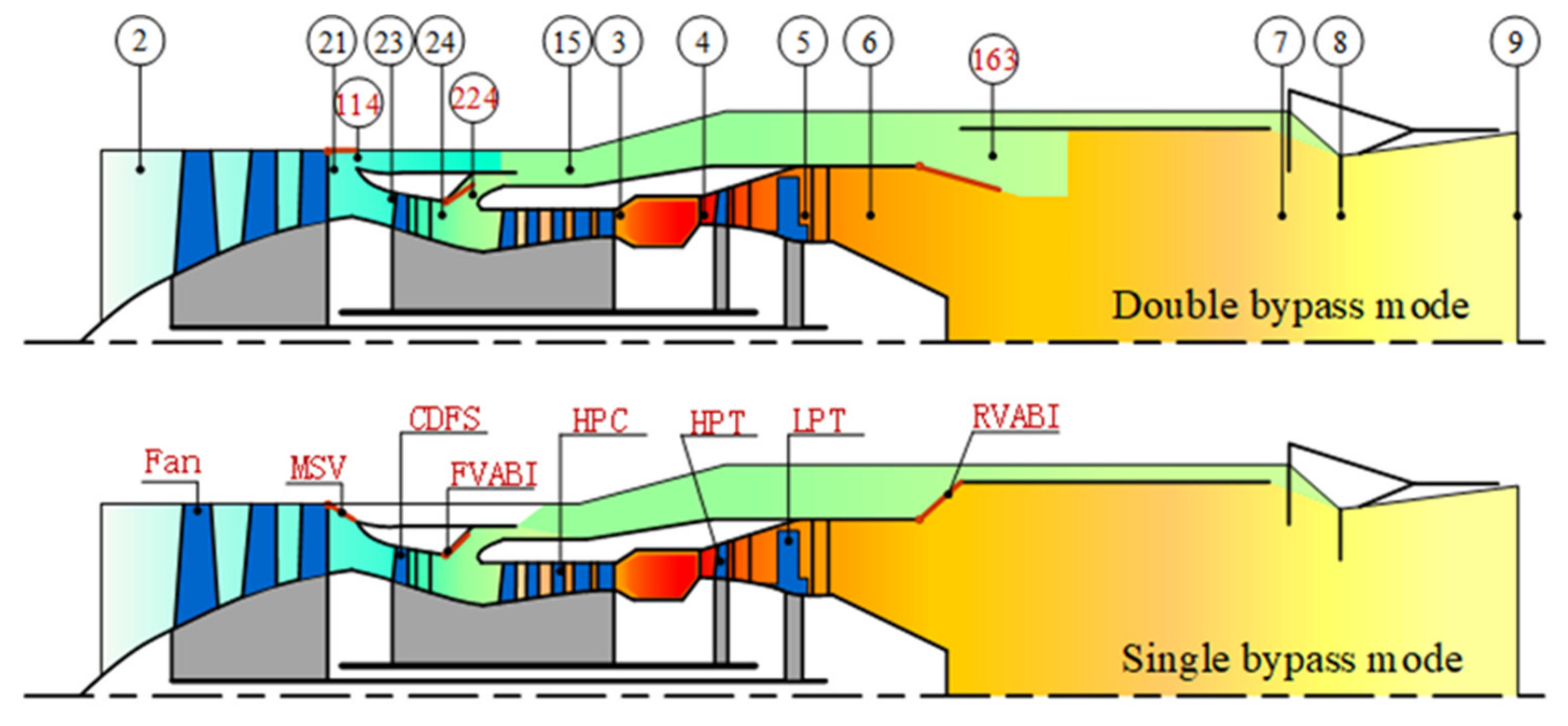
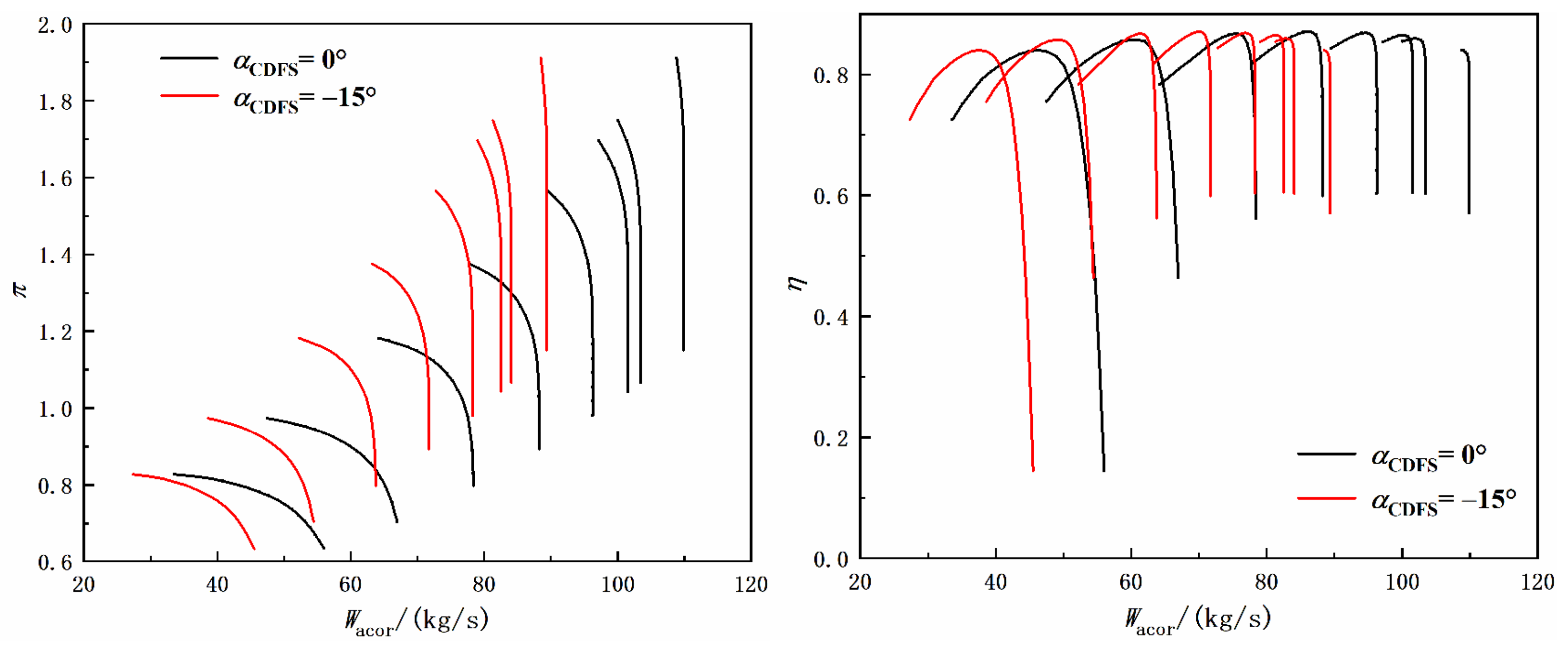
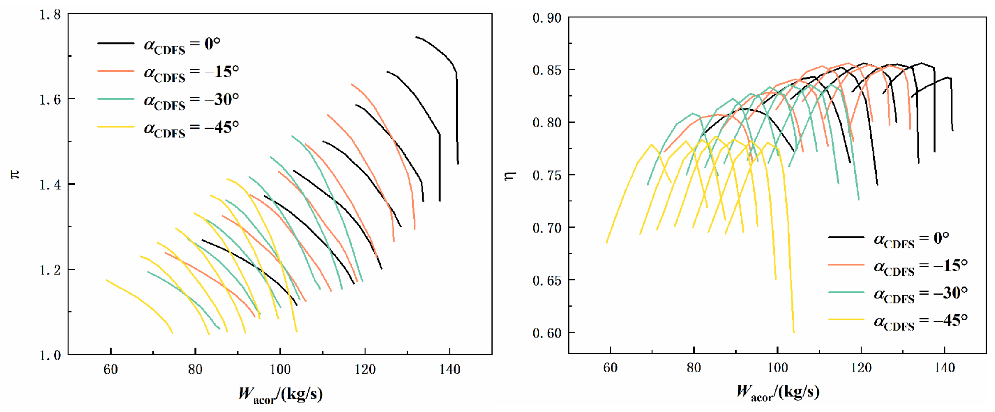
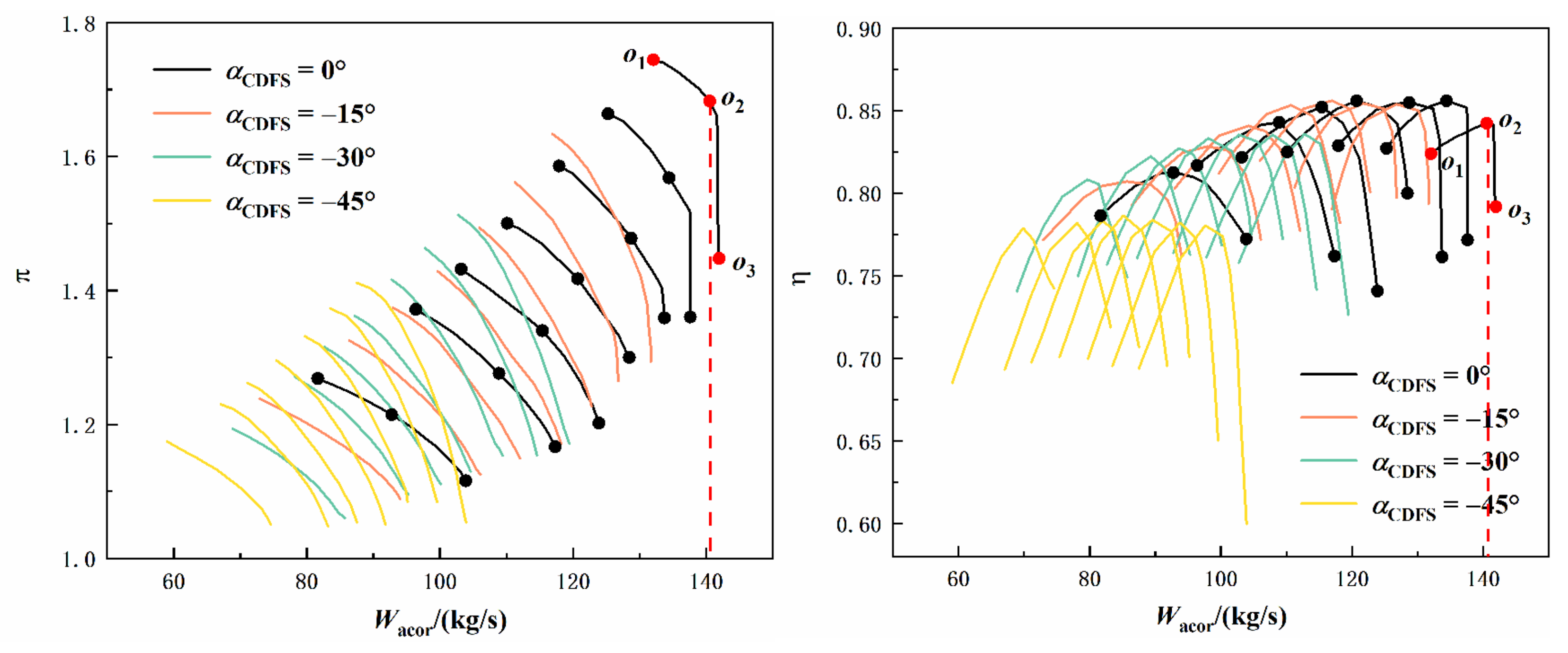
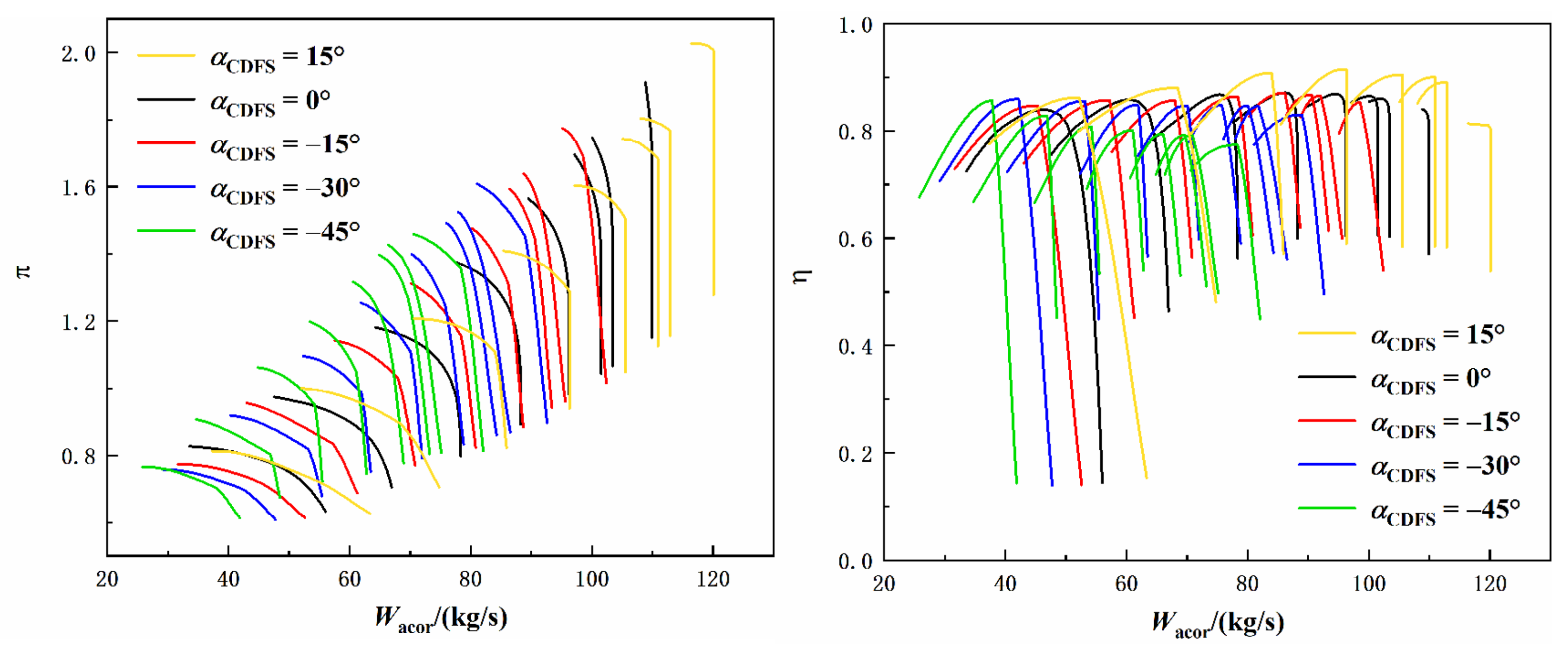
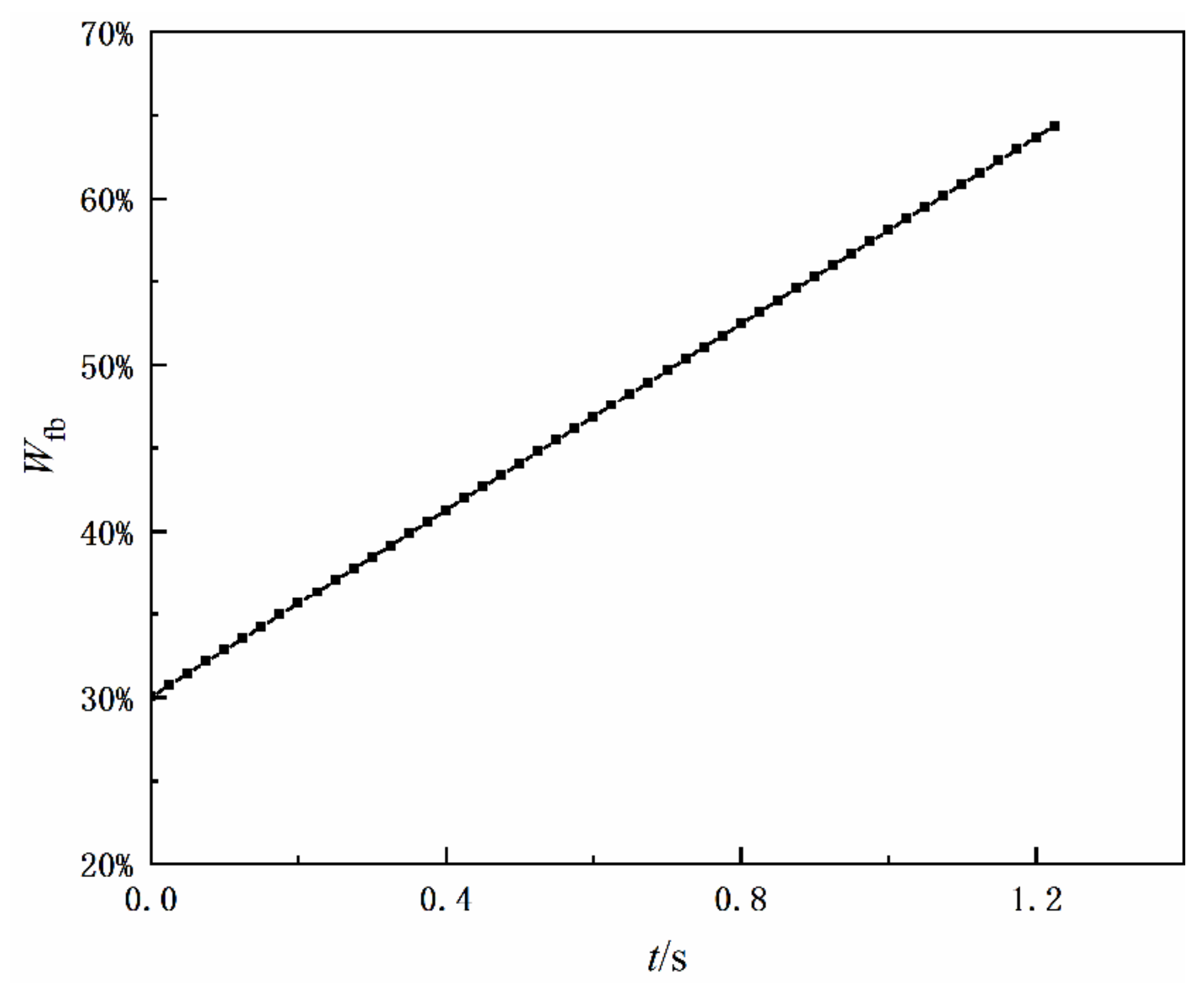
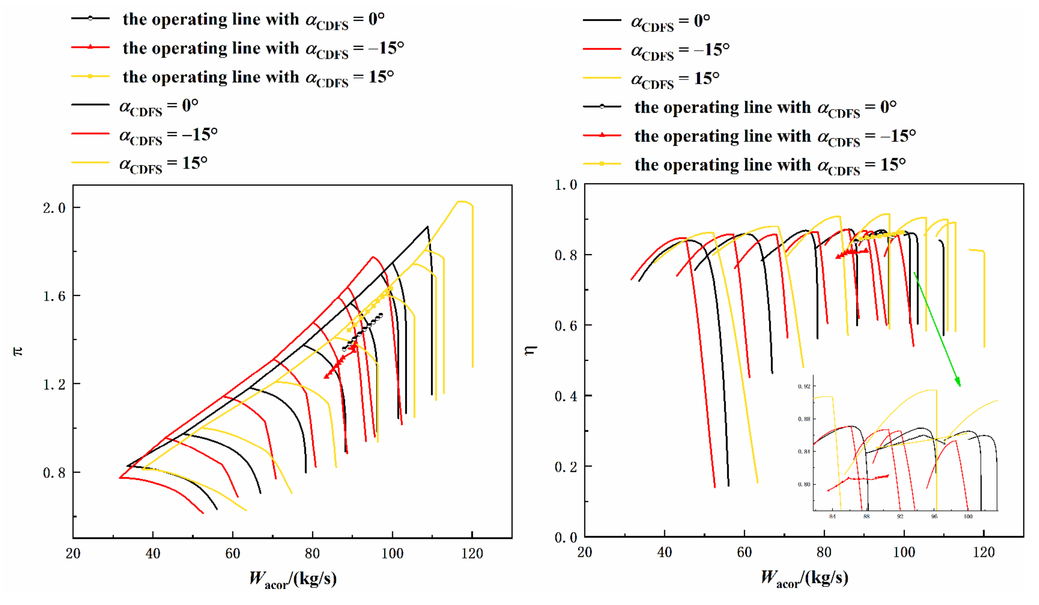
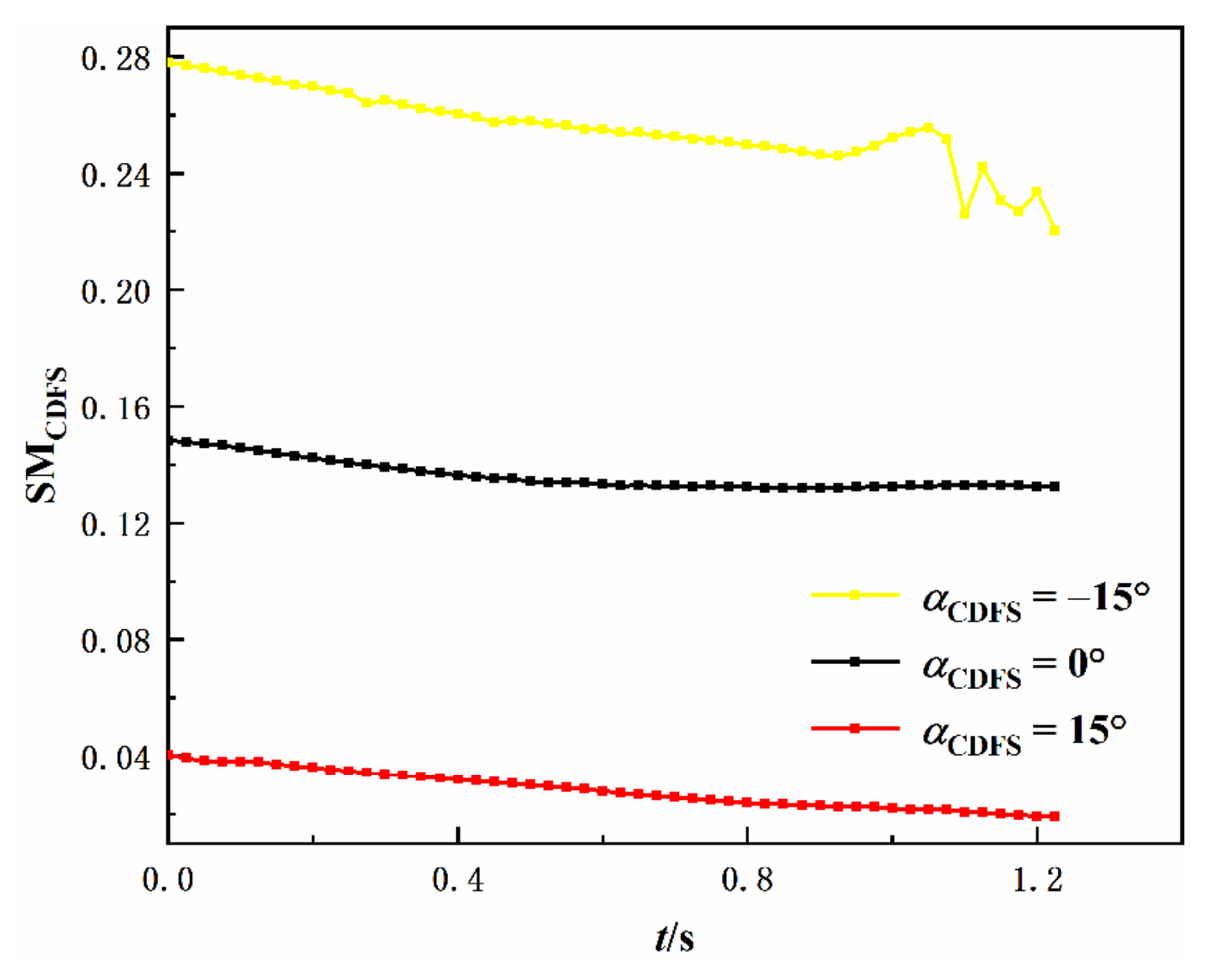
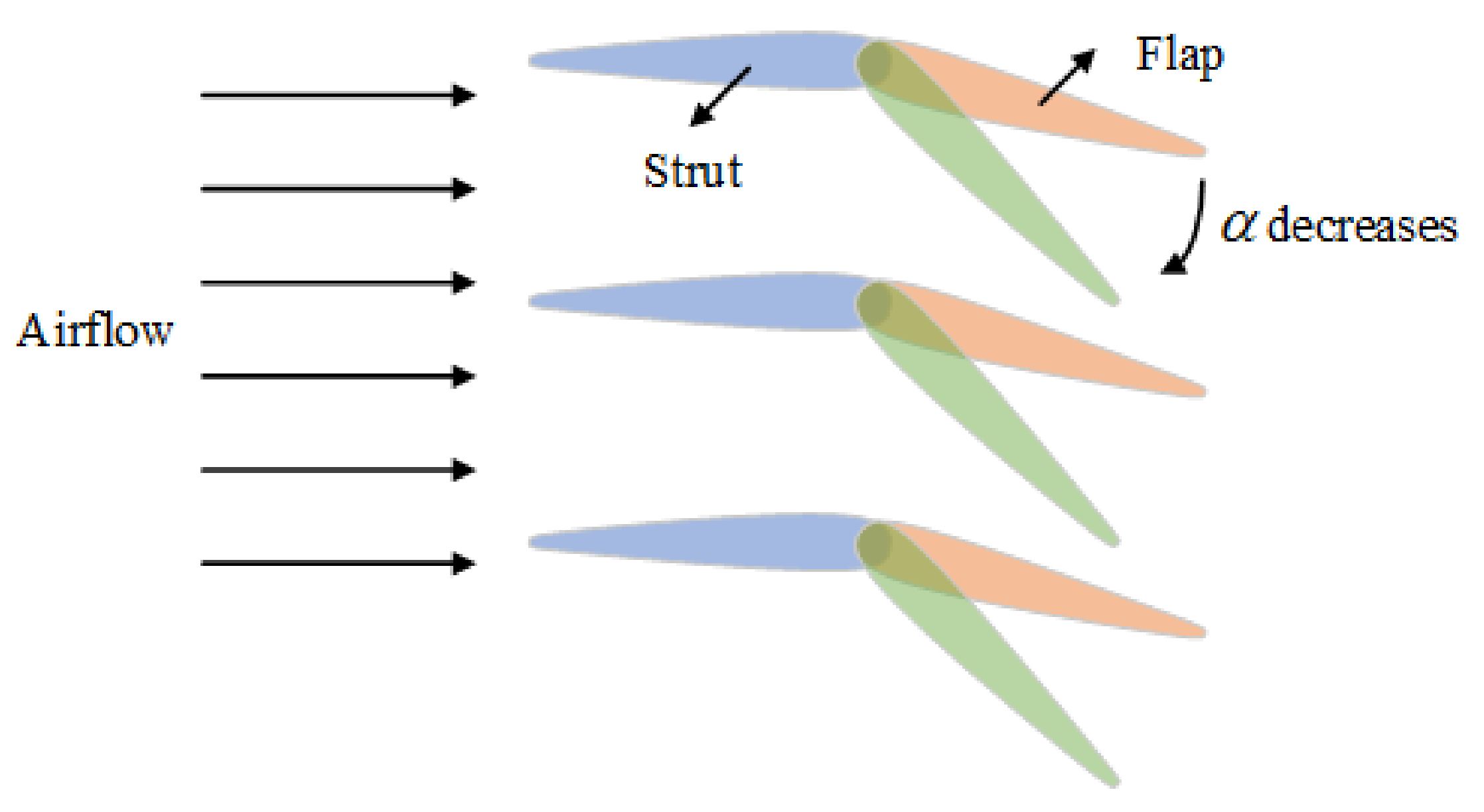
• Simulations of the acceleration process of the variable cycle engine are carried out in this paper. The results show that the designed characteristics of the CDFS can well reflect the change law of the characteristics when the geometric angle changes. When the guide vane angle changes, the component characteristics, such as surge margin, efficiency, etc., will also change accordingly. Therefore, in the subsequent design of the aeroengine control schedule, factors such as limits and performance should be comprehensively considered to determine an appropriate control schedule for the guide vane.

References

1. Nelson, D.P.; Morris, P.M. Experimental Aerodynamic and Acoustic Model Testing of the Variable Cycle Engine (VCE) Testbed Coannular Exhaust Nozzle System: Comprehensive Data Report; NASA: Washington, DC, USA, 1980. Available online: https://ntrs.nasa.gov/citations/19800017801 (accessed on 10 January 2023).
2. Willis, E.; Welliver, A. Variable-cycle engines for supersonic cruise aircraft. In Proceedings of the 12th Propulsion Conference, Key Biscayne, FL, USA, 14–17 November 1976. [Google Scholar] [CrossRef]
3. Berton, J.J.; Haller, W.J.; Seidel, J.A.; Senick, P.F. A NASA Lewis Comparative Propulsion System Assessment for the High-Speed Civil Transport. In NASA. Langley Research Center, First Annual High-Speed Research Workshop, Part 2; NASA: Washington, DC, USA, 1992. Available online: https://ntrs.nasa.gov/citations/19940028971 (accessed on 10 January 2023).
4. Szellga, R.; Allan, R.D. Advanced Supersonic Technology Propulsion System Study; SAE International: Warrendale, PA, USA, 1974. [Google Scholar]
5. Vyvey, P.; Bosschaerts, W.; Fernandez, V.; Paniagua, G. Study of an Airbreathing Variable Cycle Engine. In Proceedings of the 47th AIAA/ASME/SAE/ASEE Joint Propulsion Conference & Exhibit, San Diego, CA, USA, 31 July–3 August 2011. [Google Scholar]
6. Buettner, R.; Roberts, R.A.; Wolff, M.; Behbahani, A. Design of a Transient Variable Cycle Turbine Engine Model for System Integration with Controls. In Proceedings of the AIAA Modeling and Simulation Technologies Conference, Grapevine, TX, USA, 9–13 January 2017. [Google Scholar]
7. Wood, A.; Pilidis, P. A variable cycle jet engine for ASTOVL aircraft. Aircr. Eng. Aerosp. Technol. 1997, 69, 534–539. [Google Scholar] [CrossRef]
8. Nascimento, M.; Pilidis, P. The selective bleed variable cycle engine. In Proceedings of the ASME 1991 International Gas Turbine and Aeroengine Congress and Exposition, Orlando, FL, USA, 3–6 June 1991. [Google Scholar]
9. Murthy, S.; Curran, E.T. Variable Cycle Engine Developments at General Electric-1955–1995. In Developments in High-Speed Vehicle Propulsion Systems; American Institute of Aeronautics and Astronautics: Reston, VI, USA, 1996; pp. 105–158. [Google Scholar]
10. Song, F.; Zhou, L.; Wang, Z.; Lin, Z.; Shi, J. Integration of high-fidelity model of forward variable area bypass injector into zero-dimensional variable cycle engine model. Chin. J. Aeronaut. 2021, 34, 1–15. [Google Scholar] [CrossRef]
11. Chen, H.; Cai, C.; Luo, J.; Zhang, H. Flow control of double bypass variable cycle engine in modal transition. Chin. J. Aeronaut. 2022, 35, 134–147. [Google Scholar] [CrossRef]
12. Fishbach, L.H.; Koenig, R.W. Geneng II: A Program for Calculating Design and off-Design Performance of Two- and Three-Spool Turbofans with as Many as Three Nozzles; NASA: Washington, DC, USA, 1972.
13. Villace, V.F.; Paniagua, G. Numerical Model of a Variable-Combined-Cycle Engine for Dual Subsonic and Supersonic Cruise. Energies 2013, 6, 839–870. [Google Scholar] [CrossRef] [Green Version]
14. Lytle, J.; Follen, G.; Naiman, C.; Evans, A. Numerical Propulsion System Simulation (NPSS) 1999 Industry Review; NASA: Washington, DC, USA, 2000.
15. Patrick, M.; Nicholas, N.; Kevin, M.; Eric, W.; Joshua, C.; Soumya, P. A First Principles Based Approach for Dynamic Modeling of Turbomachinery. SAE Int. J. Aerosp. 2016, 9, 45. [Google Scholar]
16. Kania, M.; Koeln, J.; Alleyne, A.; McCarthy, K.; Wu, N. A Dynamic Modeling Toolbox for Air Vehicle Vapor Cycle Systems; SAE International: Warrendale, PA, USA, 2012; Volume 10. [Google Scholar]
17. Fang, X.; Liu, S.; Wang, P.; Zhang, W. Application of a 3D Blade Design Method for Supersonic Vaneless Contra-Rotating Turbine. In Proceedings of the ASME Turbo Expo 2008: Power for Land, Sea, and Air, Berlin, Germany, 9–13 June 2008. [Google Scholar]
18. Fang, X.; Zhao, Y.; Liu, S.; Wang, P.; Liu, Z. Research of a New Design Method of Variable Area Nozzle Turbine for VCE: Harmonic Design Method. In Proceedings of the ASME 2011 Turbo Expo: Turbine Technical Conference and Exposition, Vancouver, BC, Canada, 6–10 June 2011. [Google Scholar]
19. Sundstrm, E.; Semlitsch, B.; Mihaescu, M. Assessment of the 3D Flow in a Centrifugal compressor using Steady-State and Unsteady Flow Solvers. In Proceedings of the SAE 2014 International Powertrain, Fuels & Lubricants Meeting, Birmingham, UK, 20–23 October 2014. [Google Scholar]
20. Tsoutsanis, E.; Meskin, N.; Benammar, M. An efficient component map generation method for prediction of gas turbine performance. ASME 2014, 6, V006T06A00. [Google Scholar]
21. Tsoutsanis, E.; Khorasani, K.; Benammar, M. Transient gas turbine performance diagnostics through nonlinear adaptation of compressor and turbine maps. J. Eng. Gas Turbines Power 2015, 137, 091201. [Google Scholar] [CrossRef]
22. Pilidis, P.; Li, Y.; Newby, M.; Tsoutsanis, E. Non-linear model calibration for off-design performance prediction of gas turbines with experimental data. Aeronaut. J. 2017, 121, 1758–1777. [Google Scholar]
23. Steven, G.; Jeffrey, D.; Roy, J.; Walter, S. Compressor Performance Modeling and Prognostics Using Artificial Neural Networks. AIAA 2016-0171. In Proceedings of the AIAA Modeling and Simulation Technologies Conference, San Diego, CA, USA, 4–8 January 2016. [Google Scholar]
24. Pau, C.; Hui, W.; Soumya, S. Patnaik. Modeling of Centrifugal Compressor Performance Using Machine Learning Techniques. AIAA 2020-0134. In Proceedings of the AIAA Scitech 2020 Forum, Orlando, FL, USA, 6–10 January 2020. [Google Scholar]
25. Kurzke, J.; Riegler, C. A New Compressor Map Scaling Procedure for Preliminary Conceptional Design of Gas Turbines. In Proceedings of the ASME Turbo Expo 2000: Power for Land, Sea, and Air, Munich, Germany, 8–11 May 2000. [Google Scholar]
26. Kurzke, J. Model Based Gas Turbine Parameter Corrections. In Proceedings of the ASME Turbo Expo, Collocated with the International Joint Power Generation Conference, Atlanta, GA, USA, 16–19 June 2003. [Google Scholar]
27. Li, Y.; Ghafir, M.; Wang, L.; Singh, R.; Huang, K.; Feng, X.; Zhang, W. Improved Multiple Point Non-Linear Genetic Algorithm Based Performance Adaptation Using Least Square Method. J. Eng. Gas Turbines Power 2012, 134, 031701. [Google Scholar] [CrossRef]
28. Li, S.; Tang, H.; Chen, M. A new component maps correction method using variable geometric parameters. Chin. J. Aeronaut. 2021, 34, 360–374. [Google Scholar] [CrossRef]
29. Sullivan, T.; Parker, D. Design Study and Performance Analysis of a High-Speed Multistage Variable-Geometry Fan for a Variable Cycle Engine; NASA: Washington, DC, USA, 1979.
30. Ren, C.; Chen, Y.; Jia, L.; Zhou, C. Variable compression component interpolation method for turbine engine. In Proceedings of the 2018 9th International Conference on Mechanical and Aerospace Engineering (ICMAE), Budapest, Hungary, 10–13 July 2018. [Google Scholar]
31. Matthew, G.L.; Phillip, J.A. A Parametrization Framework for Multi-Element Airfoil Systems Using Bézier Curves, AIAA 2022-3525. In Proceedings of the AIAA AVIATION 2022 Forum, Chicago, IL, USA, 16 June 2022. [Google Scholar]
32. Satyanarayana, G.M.; David, C.; Isaac, E.W.; Dzung, M.T.; Justin, M.B.; Swaroop, D. Quadratic Bezier Curves for Multi-Agent Coordinated Arrival in the Presence of Obstacles, AIAA 2021-1879. In Proceedings of the AIAA Scitech 2021 Forum, Nashville, TN, USA, 11–15 January 2021. [Google Scholar]
Figure 1. Structure diagram of the variable cycle engine.
Aerospace 10 00196 g001
Figure 2. Characteristic maps of CDFS only multiplied by correction factor.
Aerospace 10 00196 g002
Figure 3. Characteristic maps of the maturely designed CDFS.
Aerospace 10 00196 g003
Figure 4. BP neural network topology.
Aerospace 10 00196 g004
Figure 5. Diagram of selected operating points.
Aerospace 10 00196 g005
Figure 6. Extended characteristic maps based on two-dimensional interpolation.
Aerospace 10 00196 g006
Figure 7. Surface diagram of change of offset coefficient at different operating points: (a) k π of the surge boundary point; (b) k π of the peak efficiency point; (c) k π of the stall boundary point; (d) k w of the surge boundary point; (e) k w of the peak efficiency point; (f) k w of the stall boundary point; (g) of the surge boundary point; (h) k η of the peak efficiency point; (i) k η of the stall boundary point.
Aerospace 10 00196 g007
Figure 8. Schematic diagram of the Bezier curve of order 3.
Aerospace 10 00196 g008
Figure 9. Comparison between the characteristic map generated by Bezier curve optimization and the original characteristic map.
Aerospace 10 00196 g009
Figure 10. Characteristic maps of the DCDFS.
Aerospace 10 00196 g010
Figure 11. Variation curve of fuel flow rate during acceleration.
Aerospace 10 00196 g011
Figure 12. Variation diagram of engine operating points when the guide vane angle of CDFS changes.
Aerospace 10 00196 g012
Figure 13. Surge margin of CDFS under different guide vane angles.
Aerospace 10 00196 g013
Figure 14. Schematic diagram of guide vane angle change.
Aerospace 10 00196 g014