Abstract
Radiographic testing is generally used in the quality management of aeroengine turbine blades. Traditional radiographic testing is critically dependent on artificially detecting professional inspectors. Thus, it sometimes tends to be error-prone and time-consuming. In this study, we gave an automatic defect detection method by combining radiographic testing with computer vision. A defect detection algorithm named DBFF-YOLOv4 was introduced for X-ray images of aeroengine turbine blades by employing two backbones to extract hierarchical defect features. In addition, a new concatenation form containing all feature maps was developed which play an important role in the present defect detection framework. Finally, a defect detection and recognition system was established for testing and output of complete turbine blade X-ray images. Meanwhile, nine cropping cycles for one defect, flipping, brightness increasing and decreasing were applied for expansion of training samples and data augmentation. The results found that this defect detection system can obtain a recall rate of 91.87%, a precision rate of 96.7%, and a false detection rate of 7% within the score threshold of 0.5. It was proven that cropping nine times and data augmentation are extremely helpful in improving detection accuracy. This study provides a new way of automatic radiographic testing for turbine blades.
1. Introduction
To improve aeroengine efficiency and reach aircraft performance requirements, the environment for engine parts, particularly engine blades, has become increasingly strenuous. Safety and reliability in operation have long been a concern in industry and academia. However, in the aeroengine turbine blades casting process, internal defects such as slag inclusion, remainder, broken core, gas cavity, crack and cold shut are apt to occur inevitably [1,2]. In addition, turbine blades usually work under strenuous conditions of high pressure, high temperature and high speed for a long time. If internal defects go undetected, they are likely to produce stress concentrations and cause fracture failure, leading to flight accidents [3,4]. To avoid such problems, quality management for turbine blades is essential before they leave the factory.
Nondestructive testing is an inevitable part of the investment casting turbine blade quality management. Conventional nondestructive testing methods include eddy current testing, magnetic particle testing, radiographic testing, ultrasonic testing, isotopic photography, penetrant testing, infrared thermography, and noise testing [5,6,7]. These methods use auxiliary tools to detect defects and rely on human subjective judgment. They are a semiautomatic detection means. For example, the recognition and classification of defects depend on visual observation of X-ray images obtained from radiographic testing, which always tends to be error-prone and time-consuming. However, with the rapid development of the aviation industry and increasing production demands, conventional nondestructive testing faces tremendous pressure and challenges.
Many scholars devote themselves to the automation and intellectualization of defect detection. Most of these methods are based on computer vision technology for defect detection [8]. In recent years, deep learning has performed well in defect detection [9,10,11,12] and segmentation [13,14,15,16] in many industrial fields. These defect recognition and classification methods based on deep learning learn and extract defect features from a large number of defect samples, and their detection performance has greatly outperformed traditional manual feature extraction methods [17,18,19]. Applying computer vision technology to X-ray images is an effective method for realizing the intellectualization of radiographic testing. Mery et al. [20] are devoted to a variety of computer vision methods based on a self-built X-ray image dataset called GDXray. They compared and studied 24 computer vision techniques, including deep learning, local descriptors, sparse representations and texture features, among others, by using GDXray datasets of cropped X-ray images in automotive components [21]. Ferguson et al. [22,23] adopted transfer learning to train different backbones and object detection models, including VGG16 [24], residual network (ResNet-101) [25], Faster R-CNN [26] and single-shot multibox detector (SSD) [27], based on GDX-ray datasets [20], and evaluated and compared their performance for defect detection of X-ray images in industrial castings. Fuchs et al. [28,29] trained and tested different deep learning models [30,31] based on simulated data in cast aluminum parts. Du et al. [32,33] used a feature pyramid network (FPN) [34] to extract features from X-ray images of automotive aluminum casting parts and further improved the performance of the defect detection and recognition system by utilizing the RoIAlign algorithm [35]. Wu et al. [36] adopted feature engineering and machine learning methods to study computed aided detection of casting defects in X-ray images. The above research focuses on automatic radiographic testing using state-of-the-art computer vision technology. In addition to applying deep learning to the detection of X-ray images, the deep learning method is also applied to aircraft engine borescope inspection [37,38,39]. However, there are few reports on the application of deep learning to defect detection for X-ray images of aeroengine turbine blades. In this paper, deep learning is applied to the radiographic testing of aeroengine turbine blades. We aim to utilize a considerable number of X-ray images with defects to learn defect characteristics and realize the automatic recognition and location of defects (automation and intelligence of radiographic detection). The main contributions of this study are summarized as follows:
- (1)
- We propose a novel dual backbone detection framework based on a one-stage object detection algorithm for aeroengine turbine blade X-ray images by employing two DCNNs to extract hierarchical defect features.
- (2)
- We design a novel concatenation form containing all feature maps to build a PAN (path aggregation network). The PAN we build, as the neck of the defect detection model, fuses different scale feature maps, enhances valid feature propagation, and ensures defect detection performance.
- (3)
- We adopt nine cropping cycles for one defect and employ image preprocessing and data augmentation techniques such as rotation, flipping, and brightness increasing and decreasing, which greatly expands the training dataset and significantly improves the defect detection model accuracy.
The remainder of this paper is outlined as follows: In Section 2, we introduce one-stage and two-stage object detection algorithms based on deep learning in detail by taking classical object detection algorithms (Faster R-CNN and YOLOv3) as examples in computer vision. In Section 3, we illustrate the framework and details of our method. Section 4 describes the relevant parameter settings and details of the experiments (model training and testing). The results are demonstrated and discussed in Section 5. Finally, Section 6 presents the conclusions and further work.
2. The Object Detection Algorithm on Deep Learning
The object detection algorithm is a basic algorithm generally used in the computer vision field. It combines region selection and image classification. The purpose of object detection is to classify objects in images or videos and give their location information. Therefore, the main task includes two parts: object classification and object location. Figure 1 shows the object detection implementation process. In the traditional object detection algorithm, a sliding window is utilized to obtain candidate regions, feature extraction is performed manually, and traditional classifiers are used for classification. The accuracy and its real-time performance are relatively low. As shown in Figure 1, the red dashed box represents the traditional image processing, and the yellow filled box below represents the image processing by CNNs. The success of CNNs in classification as in AlexNet has led to their adoption in object detection. Because of learning features by deep neural networks, image feature extraction is more effective, which brings higher accuracy, real-time performance of object detection and increasingly wide utilization in all fields. Object detection algorithms based on deep learning are divided into two-stage algorithms and one-stage algorithms according to the differences in the structure and process.

Figure 1.
Object detection implementation process.
The process of object detection with a two-stage algorithm goes through two steps. First, rough classification and location of objects are carried out based on the main features extracted by the backbone. In this process, a large number of region proposals containing foreground (object) and background are obtained. The second step is to select some images with high confidence scores in these region proposals for final thorough object classification and location. The intersection over union (IoU) is a typical indicator for judging goals or background in region proposals, which is the overlap ratio between the ground-truth box and the region of proposal, as shown in Figure 2.
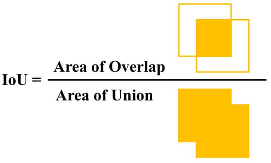
Figure 2.
Illustration of IoU.
The typical two-stage algorithm for object detection is Faster R-CNN, which includes four contents as follows [26]: 1. Main feature extraction. 2. Proposals acquisition by RPN (region proposal network). 3. ROI pooling for cropping proposal feature maps. 4. Image classification and bounding box regression for output. The implementation process is shown in Figure 3.
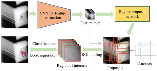
Figure 3.
Faster R-CNN implementation process.
Compared with the two-stage object detection algorithm, the one-stage object detection algorithm directly predicts the object category and location. The framework of the algorithm is relatively simple. This end-to-end detection method makes it more advantageous in detection speed. There are several typical algorithms within one stage, such as SSD (single-shot multibox detector) [27] and YOLO (you only look once) series [40].
Figure 4 shows the network structure of the YOLOv3 algorithm. The DBL (represented as DarknetConv2d_BN_Leaky in the code) in the figure is the basic component of YOLOv3, and its structure is composed of convolution (Conv), batch normalization (BN), and the leaky ReLU activation function. The Res_unit in the figure is a residual unit composed of two DBL connected. Res-n represents a residual connection block, which is successively connected by zero-padding, DBL and N Res_unit residual units and has the function of downsampling the input image. DRRR is the main feature extraction network used by YOLOv3, which consists of a DBL followed by three residual connection blocks. YOLOv3 is one of the most popular object detection algorithms. The concrete realization of YOLOv3 algorithm can refer to [40].
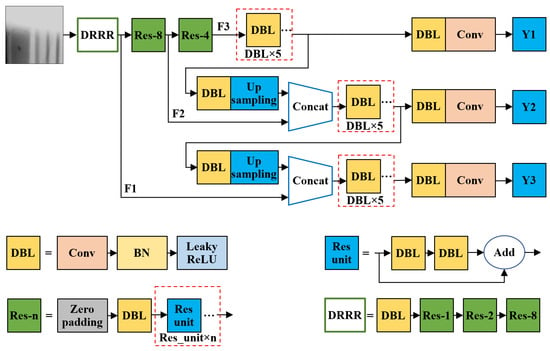
Figure 4.
Network structure of the YOLOv3 algorithm.
3. The Deep Learning Method of Defect Localization and Recognition for Turbine Blades
In this study, the implementation process of the detection method we proposed can be described by four parts. First, X-ray images of defective turbine blades are accessed and preprocessed for the building training set, validation set, and testing set. Next, a defect detection model for turbine blades is built, which adopts dual backbone networks for feature extraction, a feature pyramid network (FPN) and a path aggregation network (PAN) for feature fusion and is based on one-stage object detection. Moreover, the objective function (also called the loss function) and weight optimization algorithm are determined for model training. Then, the model training process is performed by utilizing the training set and validation set based on the gradient descent method. Finally, the defect detection model is tested on the testing set. The details of implementation for each section are given below.
3.1. X-ray Image Acquisition and Preprocessing
3.1.1. Defect Samples and Labels
Deep learning for image recognition is generally pure data-driven, and the training data have a great impact on the prediction accuracy of the model. However, high detection accuracy not only requires that the number and coverage of training data be large enough but also requires that the corresponding label data be accurate. With the help of an aviation manufactory, we collected 600 X-ray films containing defective turbine blades with a size of 0.5 m × 0.5 m. There were 50 turbine blade images on each film, in which scattered defective blades are hidden. To obtain high-resolution X-ray digital images of aeroengine turbine blades, the original films were scanned with an industrial film digital scanner using optimal resolution scanning parameters. The size of each X-ray image scanned from the original film was 7960 × 9700. Figure 5 shows the process to obtain X-ray film digital images with an industrial film digital scanner. The industrial film digital scanner was connected to a computer. After automatic scanning, these images were corrected, marked, and saved manually as X-ray film digital images. Figure 6 shows an X-ray film digital image and a defective turbine blade sample with a locally enlarged region of defects. We cropped defective turbine blade images with the identical pixel size (770 × 1700) from the X-ray film digital image. Finally, 2137 X-ray images of turbine blades with defects were obtained as the defect sample dataset of this study.
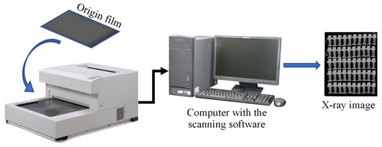
Figure 5.
X-ray film digital image acquisition process.
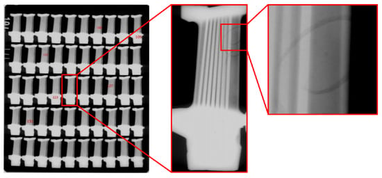
Figure 6.
Example of an X-ray film digital image and a defective turbine blade sample with a locally enlarged region of defects.
In the process of model training based on deep learning, the information of defect category and location on each training sample should be given in advance by manual evaluation as a training objective. Based on edge smoothness, end sharpness, trend change rate, relative position, symmetry, included angle, length to short axis ratio, and gray relative change rate, the main characteristics of six kinds of defects were analyzed and evaluated by fuzzy reasoning. The six kinds of defects were slag inclusion, remainder, broken core, gas cavity, crack and cold shut, which are all internal defects. Slag inclusion, remainder, and broken core are all inclusion defects. It looks like there are slag inside of metal castings. Slag inclusion is low-density inclusion, and remainder and broken core are high-density inclusion. Gas cavity is a kind of cavities defect. Gases are entrapped by solidifying metal on the inside of the casting, which results in a rounded or oval blowhole as a cavity. The crack of castings can divided into hot crack and cold crack, which are caused by a variety of factors [41]. Some cracks are very obvious and can be easily seen with the naked eye. Other cracks are very difficult to see without magnification in radiographic testing. Cold shut is also called cold lap. It is a crack with round edges. Cold shut is because of a low melting temperature or a poor gating system. Figure 7 presents these different kinds of defects. These defect X-ray images were categorized and labeled by certified and experienced NDT engineers. We found that approximately 12% of the pseudo defects in X-ray images were caused by the film itself and the film digitization process, and these pseudo defects were considered as non-defects. For each defective turbine blade picture, label data, including the defect category and the vertex coordinates of defect rectangular area (, , , ), were determined by labeling software. To date, training and label datasets containing 2137 samples with six kinds of defects were obtained for model training. Table 1 shows the statistical results of the defect samples.
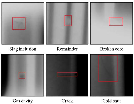
Figure 7.
Examples of different kinds of defects.

Table 1.
Statistical results of defect samples.
3.1.2. Image Preprocessing and Data Augmentation
The pixel size of most defects is smaller than , which is extremely small compared with the pixel size of the turbine blade. This large scale difference makes it almost impossible to directly input the turbine blade image for defect detection. In our detection method, each turbine blade image was cut to a fixed size first. Then, these local images of the turbine blade were detected in turn. Finally, the mosaic of the complete turbine blade from these local images was output for visualization. Based on experience, we cropped the defect image with a size of from each defective turbine blade image. Each defective turbine blade image was cropped nine times in the defect region such that the defect falls evenly on the cropped image of fixed size, as shown in Figure 8. The corresponding label data were revised simultaneously. This process expanded the number of original defect samples to nine.
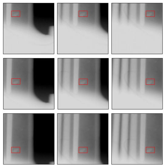
Figure 8.
Example of cropped pictures obtained by nine cropping cycles in defective turbine blade images.
Data augmentation is an effective means to improve the prediction accuracy of deep learning models. Images can be either flipped or rotated for data augmentation. In this study, each cropped picture was flipped or rotated counterclockwise by 90 degrees with a 50% probability, and the brightness was randomly increased or decreased by 20%. All data augmentation methods were applied to the training datasets, and testing images were kept in their original states all the time. Figure 9 depicts our data augmentation examples.
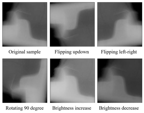
Figure 9.
Examples of image data augmentation.
3.2. Network Structure of the Defect Detection Model Based on Deep Learning
In addition to the training and label data, network structure is a crucial factor in determining the performance of the deep learning model. Our defect detection model made of a deep neural network, called DBFF-YOLOv4 (dual backbone feature fusion YOLOv4), is composed of four modules (as shown in Figure 10). The first module is the dual backbone feature extraction networks named ResNet-50 and CSPDarknet-53, which are responsible for generating feature maps with different scales. The second module, called the neck, is composed of a feature pyramid network (FPN) and a path aggregation network (PAN), which adopt a novel concatenation form between different scales and different backbone feature maps for feature fusion. The third module is the head, which is identical to that of YOLOv3 (as shown in Figure 4). The last module is coordinate correction and NMS for final detection results. The entire system is a single, unified network for defect detection of turbine blades. Using a dual backbone and a concatenation structure, sufficient defect semantic information and location information are captured. In the first part of this section, we introduce the dual backbone feature extraction networks with their different scale feature maps. In the second part, we present the details of PAN with a novel concatenation form. In the third part, we demonstrate defect prediction in the model head and the final outputs of the detection results.
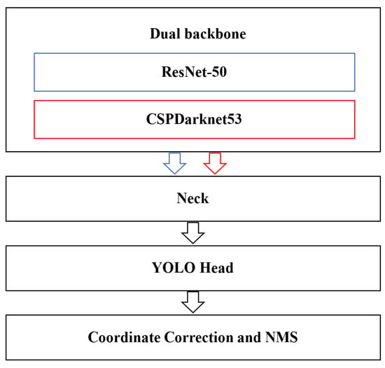
Figure 10.
Defect detection model framework.
3.2.1. Dual Backbone Networks for Feature Extraction
We adopt ResNet-50 and CSPDarknet53 as the dual backbone networks of our model. In ResNet-50, the last three layers (pooling, full connection and softmax) are removed. Table 2 shows the framework of ResNet-50 without the last three layers, where the square brackets represent the bottleneck blocks. Figure 11 shows two kinds of bottleneck frameworks composed of three convolutional layers named Conv Block and Identity Block. In both blocks, the shortcut connections simply perform one conv or identity mapping, and their outputs are added to the outputs of the stacked layers. Conv mapping with a stride size of 2 halved the size of the input feature map. Therefore, in many stacked blocks, downsampling is performed by the Conv Block first. The stacked layers are composed of three convolutional layers with filter sizes of , and . The layers are responsible for reducing and then increasing dimensions, leaving the layer with smaller input/output dimensions. Batch normalization and linear rectification activation functions (ReLUs) are used in the bottleneck block. Three feature maps are output after Conv3_4, Conv4_6, and Conv5_3, called F1, F2, and F3.

Table 2.
The framework of ResNet-50 without the last three layers.
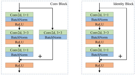
Figure 11.
Two kinds of bottleneck frameworks (left: Conv Block, right: Identity Block).
CSPDarknet53 is the backbone of YOLOv4, which employs a CSPNet strategy to partition the feature map of the base layer into two parts and then merge them through a cross-stage hierarchy. In CSPDarknet53, the first stacked layers are composed of convolution, batch normalization, and Mish activation functions (as shown in Equation (1)). Downsampling is performed after each stacked block is composed of several ResBlock bodies with the CSPNet strategy. After that, the SPP-block is used to enhance the receptive field. The whole CSPDarknet53 outputs three feature maps with different scales, called P1, P2, and P3. Figure 12 shows the structure of CSPDarknet53 and its output feature maps.
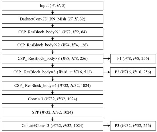
Figure 12.
The structure of CSPDarknet53 and its output feature maps.
3.2.2. PAN with a Novel Concatenation Form for Feature Fusion and Propagation
For six feature maps output from two backbones, a novel concatenation form containing all feature maps is proposed to construct a PAN. Our PAN, as the neck of the defect detection model, is conducted to fuse different scale feature maps to improve performance. Figure 13 demonstrates the structure of our PAN. The inputs are six feature maps that are divided into three hierarchies. F1 and P1 are the largest feature maps from the shallow layer output of ResNet-50 and CSPDarknet53, respectively. Similarly, F2 and P2 are feature maps from the middle layer output of ResNet-50 and CSPDarknet53, and F3 and P3 are the smallest feature maps from the last layer output of the above two backbone networks. F3 and P3 containing semantic information of the larger receptive field are concatenated with P2 and F2 after performing upsampling, respectively. Then, identical upsampling and concatenation are performed on medium feature maps obtained in the previous concatenation and the largest feature maps. It is worth noting that the bottom-up process is a dual path since there are two sets of backbone feature maps. In the bottom-up process, the top-level mapping is obtained by concatenating the last outputs of the two previous bottom-up paths. At this point, one bottom-up path is performed to fuse features from different features and hierarchies. After the bottom-up process, PAN outputs fusion feature maps of three scales. Here, each fusion feature map is used to predict defects of different sizes.
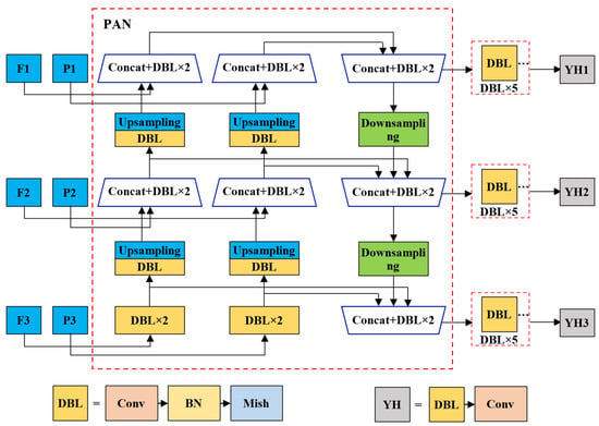
Figure 13.
The structure of our PAN.
3.2.3. Defect Prediction and Final Outputs
After PAN, five DBL layers (convolution followed by batch normalization and the mish activation function) are performed, as shown in Figure 13. In the head module, the structure is identical to that of YOLOv3. The output of the head is three arrays with dimensions of , which can be regarded as three feature maps with W width, H height, and C number of channels. Here, the subscript i refers to three hierarchies of defect detection, , and . In addition, 3 refers to the number of predicted bounding boxes, 4 contains the location information of defects, 1 is the confidence score of defects, and 6 presents the type of defects. The regression of defect location coordinates is similar to YOLOv3. First, the revised values of the coordinates relative to the anchor are output, and then the predicted coordinates of the defect are obtained based on the anchor we designed in advance. We designed nine anchors by utilizing the K-means algorithm. Three large anchors are used for YH1, three medium-sized anchors are used for YH2, and the last three small anchors are applied to YH3. Therefore, each output contains prediction boxes. The model outputs predicted bounding boxes in total. Finally, NMS is applied to obtain the final prediction results.
3.3. Objective Function
The object function (also called the loss function) of our defect detection model is identical to that of YOLOv3, which is composed of three parts: the coordinate prediction error, the intersection over union (IoU) error, and the classification error. In coordinate error, it is worth noting that the goal of location regression is the expected revised value relative to the anchor rather than the real coordinate. The total loss is defined as follows:
where indicates that the target is detected by the jth bounding box of grid i. In a predicted output hierarchy, indicates the number of grids, and B is the number of anchors per grid. If a real box is closest to the jth bounding box of grid i, and is equal to 1 at this point; otherwise, it is 0. The meaning of is the opposite of . The first two terms of the expression above are coordinate errors, in which , , , and are four revised values of the predicted box relative to the anchor corresponding to grid i, and , , , and are four real revised values. Terms 3 and 4 indicate the IoU error, in which and are the predicted confidence score and real confidence score () in grid i, respectively. The last term represents classification error, in which refers to the predicted value of the probability of the object in grid i belonging to class c, and is the real value. Except for coordinate error, which adopts the mean square error, the others adopt the binary cross-entropy loss , which is defined as follows:
3.4. Weight Optimization Algorithm
The weight optimization algorithm of deep learning is a gradient descent method based on backpropagation. The weight updated in the next step can be obtained by subtracting the product of the gradient and the learning rate from the current weight. Equation (4) gives the expression for optimizing the network weight by the gradient descent method:
where refers to the network weights, and is the learning rate. Since more than one image (a batch) is input to the network each time, to comprehensively consider the loss of each batch, the batch gradient descent algorithm is generally used; that is, the average gradient is calculated by using the whole training set of each batch. Adaptive moment estimation (Adam) [42] for stochastic optimization proposed by Diederik et al. is widely utilized in the field of image recognition, which can adjust the learning rate adaptively and can consider the cumulative effect of the gradient by introducing first and second gradient moments. Hence, we also use Adam for the optimization of our defect detection model.
4. Experiments
4.1. Model Training and Testing
We selected the Keras framework for modeling in this work. Eighty percent of the samples were used for training, and the remaining samples were used for testing. Ten percent of the training set was divided for model validation in every training epoch. Both model training and testing were performed on a Windows system with an NVIDIA GeForce GTX 2080Ti GPU. The training is divided into two stages. First, YOLOv4 with the backbone of ResNet-50 and CSPDarknet53 were pretrained on our training set. The training epoch was set to 100, and early stopping was defined when the validation loss in six consecutive epochs did not decrease. A batchsize was set to 32 in each iteration. The adaptive momentum estimation (Adam) algorithm was adopted to optimize network weights by backpropagation, in which the initial learning rate was 0.001, and the exponential decay rates (, ) were 0.9 and 0.999. Then, our model was trained, in which the initial weights of the dual backbone are from that of the pretrained YOLOv4 model in the first training stage. In the beginning of our model training, two backbones were frozen, and the neck and head of the whole model were trained by using the same parameter settings as the pretrained stage. After that, all layers were unfrozen to train in detail for 50 epochs with a batch size of 8, and the initial training rate was set to 0.0001. The learning curve of DBFF-YOLOv4 model is shown in Figure 14.
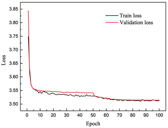
Figure 14.
The learning curve of the DBFF-YOLOv4 model.
4.2. Evaluation Criterion
Precision and recall are common indicators for most object detection models of machine learning. We also use precision and recall for the defect detection model we proposed in this study, which are defined as follows:
where TP, true positive, indicates the number of ground-truth defects that are correctly detected as defects. FP, false-positive, represents the number of false bounding boxes predicted that are actually defect-free. FN, false negative, indicates the number of ground-truth defects that are detected as nondefects, which means the number of defects missed by the model. Table 3 clearly shows the meaning of these parameters, in which the row indicates the true attributes of the sample, the list shows testing results, 1 represents defective, and 0 is nondefective. Therefore, precision is for the testing results of the model and means the correct proportion of all defects predicted in the model. Recall is for real defective samples, which indicates the proportion of defects detected from all defective samples. High precision indicates high correctness of the detection results, while high recall shows that fewer defects are missed during the detection.

Table 3.
Four possible detection results in testing.
For defect detection, a bounding box and a confidence score are generated for defect location and recognition. The intersection over union (IoU) between the predicted bounding box and the ground-truth box is used for judging right or wrong, namely, TP or FP in the detection results. Generally, the detection result with IoU > 0.5 is TP; otherwise, it is FP. A set of corresponding precision and recall values can be obtained by defining different confidence scores. The curve drawn with precision as the y-coordinate and recall as the x-coordinate is called the precision–recall curve.
In this study, the AP (average precision) was used to evaluate the defect detection performance of the model. It is calculated by interpolating the (precision) at each level R (recall), taking the maximum precision whose recall value is greater or equal than , and as shown in Equation (7):
Finally, mAP (mean average precision) for all classes is calculated by Equation (9) to evaluate the model performance:
Here, indicates the number of all defect classes (), and is the AP of class i.
5. Results and Discussion
In this section, we adopt the commonly used indicators mAP, recall, and precision to evaluate the defect detection model we proposed in this study. In addition to training and testing our model, we also built and trained YOLOv4 [43] by utilizing our defective blade images with the raw input size, . We used 427 defect samples for testing. Table 4 gives the details of the testing sets. The comparison results of the proposed DBFF-YOLOv4 and YOLOv4 with the raw input size are presented in Table 5. The results show that the DBFF-YOLOv4 we built in this study has obvious advantages for defect detection of aeroengine blades; its mAP is up to 99.58%, and the average recall within the score threshold of 0.5 is up to 91.87%. The performance of DBFF-YOLOv4 in mAP, precision, and recall significantly improved compared with YOLOv4.

Table 4.
Details of the test datasets.

Table 5.
The comparison results of DBFF-YOLOv4 we proposed and YOLOv4 with the raw input size.
To evaluate the performance of the DBFF-YOLOv4 framework on defect feature extraction, the YOLOv4 framework with different backbones was built and trained for comparison by applying our defect cropping method and data augmentation. The image input size remains in all models. All models were tested with the same testing set. We evaluated five models, in which four models for comparative research were built based on the YOLOv4 framework with the backbones of VGG16, ResNet-50, ResNet-101 and CSPDarknet-53. The results are exhibited in Table 6, Table 7 and Table 8. The comparison results of AP, mAP, and FPS in Table 6 show that our defect detection framework DBFF-YOLOv4 has the optimal performance, with a 1.54% improvement in mAP compared with the YOLOv4 framework with the backbone of CSPDarknet-53 (AP for remainder improved 0.174%, broken core improved by 0.03% and cold shut improved by 9.09%). The AP of our framework in the broken core, gas cavity, crack, and cold shut was up to 100%. Although the detection time consumption increased (37.32 ms vs. 25.86 ms), the improvement of accuracy is desirable for the quality management of aeroengine blades. These results demonstrate that our defect detection framework DBFF-YOLOv4 outperformed the others. In four models based on the YOLOv4 framework, the model with the backbone of ResNet-101 has the most layers and the lowest performance. The possible reason is that too many layers lead to overfitting.

Table 6.
The comparison results of AP, mAP, and FPS on different defect detection frameworks.

Table 7.
The comparison results of recall on different defect detection frameworks.

Table 8.
The comparison results of precision on different defect detection frameworks.
The comparison results of recall and precision in Table 7 and Table 8 show that our DBFF-YOLOv4 model outperformed the other models in average recall and precision. Compared with the YOLOv4 framework using the backbone of CSPDarknet-53, our model gained 1.46% and 0.7% improvement in recall of slag inclusion and remainder when the score threshold was 0.5, and the precision on slag inclusion and remainder improved by 0.06% and 1.54%. It is worth noting that the precision of our model on the remainder, broken core, gas cavity crack, and cold shut was up to 100% when the score threshold is 0.5, and the average precision for all defects was 99.9%.
We further studied the effectiveness of our cropping method and data augmentation on the detection performance of our DBFF-YOLOv4 model. Table 9 shows the mAP, average precision, and recall of DBFF-YOLOv4 using our cropping method and data augmentation. The results show that the mAP, average precision, and recall of DBFF-YOLOv4 significantly improved by using our cropping (nine cropping times) and data augmentation. This is especially true for nine cropping times, which expanded the number of the dataset to 9 times, and with 59.19%, 27.01% and 62.49% improvement in mAP, average precision and average recall, respectively. Our data augmentation (rotation, flipping, brightness increasing and decreasing) is also effective at improving the prediction accuracy of model detection and classification. The results show that the mAP of our model using only nine cropping times was 97.05%, and it reached 99.58% if using data augmentation based on this, with an improvement of 2.53%.

Table 9.
The comparison results of mAP, average precision, and recall of our model using our cropping method and data augmentation.
Although our model DBFF-YOLOv4 reached satisfactory performance for defect detection of aeroengine blades, missed and incorrect detection still exists. Figure 15 presents an example of the visual test results. The first two lines in Figure 15 exhibit the results of correct detection, in which ‘S’ refers to slag inclusion, ‘DX’ refers to broken core, ‘DYW’ refers to remainder, ‘A’ refers to gas cavity, ‘C’ refers to crack, and ‘CI’ refers to cold shut. The last two lines show the results of missed detection. The result demonstrates that our model fails to detect defects with extremely small sizes and excessively fuzzy outlines. The characteristics of these defects are extremely weak, containing little feature information, and the defects are similar to the background, which is the main reason for the failure of detection.
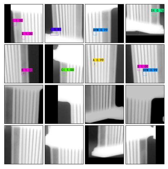
Figure 15.
Examples of visual test results.
The input of DBFF-YOLOv4 is 256 × 256 cutting images. However, it is necessary to detect a single complete blade image in real quality management of turbine blades. For this reason, an image cutting module and splicing module were added before and after DBFF-YOLOv4, respectively. A quarter size overlapping strategy of adjacent cutting pictures was used for cutting and splicing module. Finally, a defect detection and recognition system was established for testing and output of complete turbine blade X-ray images. An example of blade image cutting and splicing is shown in Figure 16. The testing process with defect detection system is as follows. First, the size of turbine blade X-ray images was calculated, and original images were padding and cutting with the size of 256×256 in cutting module. Next, the cutting pictures were input to DBFF-YOLOv4 in sequence for testing, and the results containing defect type, confidence and prediction box of each cutting picture were output visually. Finally, these cutting pictures with visual testing results were pieced into a complete turbine blade image in splicing module.
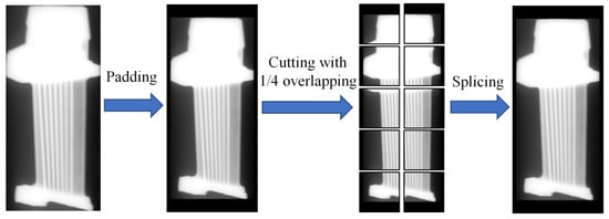
Figure 16.
Examples of blade image cutting and splicing.
We chose 527 complete X-ray images of turbine blades for the system testing, in which 427 images are defective and 100 are nondefective. The results show that the average recall of defect detection system is 91.87% within the score threshold of 0.5, which is consistent with that of the DBFF-YOLOv4 model, while its average precision is reduced from 99.9% to 96.7%. For 100 nondefective blades, the defect detection and recognition system has a false rate of 7%. An example of visual testing results for complete turbine blades is shown in Figure 17. Because the defect detection system detects the complete X-ray images of turbine blades, a large number of nondefective cutting pictures are detected additionally compared with the previous testing only using a DBFF-YOLOv4 model. Some cutting pictures of pseudo defects and similar defects may be the main reason for the high false rate of the detection system.
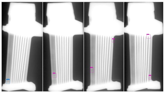
Figure 17.
Example of visual testing results for complete turbine blades.
6. Conclusions and Future Work
Radiographic testing is a general approach for quality management of aeroengine turbine blades. In this study, a new defect detection method was given by combining radiographic testing with computer vision. A dual backbone detection framework DBFF-YOLOv4 based on a one-stage object detection algorithm was developed for X-ray images of aeroengine turbine blades by employing two DCNNs to extract hierarchical defect features. In the present DBFF-YOLOv4 framework, PAN (path aggregation network) with a novel concatenation form containing all feature maps was introduced. It plays an important role in the defect detection framework for fusing different scale feature maps, enhancing valid feature propagation. The results show that the present defect detection model can obtain 99.58% mAP (with 99.9% average precision and 91.87% average recall within the score threshold of 0.5), outperforming others built by using the common object detection algorithm YOLOv4 directly. Cropping nine times and data augmentation methods greatly increased the number of samples and proved to be extremely helpful in improving the accuracy of the defect detection model, which obtained 59.19%, 27.01% and 62.49% improvements in mAP, average precision and recall, respectively. In addition, the defect detection and recognition system established for testing and visual output of complete turbine blade X-ray images can obtain a recall rate of 91.87%, a precision rate of 96.7%, and a false detection rate of 7% within the score threshold of 0.5. The present defect detection system can be applied as an auxiliary tool for manual film evaluation to improve the detection efficiency in traditional radiographic testing of aeroengine turbine blades.
The current defect detection system still exhibits missed and incorrect detection, especially for detecting defects with small sizes and fuzzy outlines. In real engineering applications, most X-ray images are non-defect. These non-defect big data were not well utilized in our model training and testing. Further work will focus on small target detection and weak feature information extraction technology, and the research of defect detection algorithm based on unsupervised deep learning for real engineering applications. In addition, generative adversarial networks (GANs) [44,45] will be studied for further data augmentation of defect samples.
Author Contributions
Methodology, D.W.; validation, H.X. and S.H.; formal analysis, H.X.; data curation, H.X.; writing—original draft preparation, D.W.; writing—review and editing, H.X.; visualization, D.W.; funding acquisition, H.X. and S.H. All authors have read and agreed to the published version of the manuscript.
Funding
This research was funded by the Science and Technology Leading Talent Program of Hunan Science and Technology Innovation Talent Program with Grant No. 2020RC4035 and the industry University Research Funding of Aero Engine Corporation of China.
Informed Consent Statement
Informed consent was obtained from all subjects involved in the study.
Data Availability Statement
The data that support the findings of this study are available from the corresponding author, Hong Xiao, upon reasonable request.
Acknowledgments
This study is supported by the Science and Technology Leading Talent Program of Hunan Science and Technology Innovation Talent Program with Grant No. 2020RC4035 and the industry University Research Funding of Aero Engine Corporation of China. The authors express great appreciation to Ke Tang and Zhifu Lin at Northwestern Polytechnical University, who participated in the discussion of this paper.
Conflicts of Interest
The authors declare no conflict of interest.
Abbreviations
The following abbreviations are used in this manuscript:
| MDPI | Multidisciplinary Digital Publishing Institute |
| YOLO | You Only Look Once |
| DBFF-YOLOv4 | Dual Backbone Feature Fusion YOLOv4 |
| VGG | Oxford Visual Geometry Group |
| R-CNN | Region-Convolutional Neural Network |
| SSD | Single-Shot multibox Detector |
| FPN | Feature Pyramid Network |
| DCNNs | Deep Convolutional Neural Networks |
| PAN | Path Aggregation Network |
| IoU | Intersection over Union |
| ROI | Region of Interests |
| RPN | Region Proposal Network |
| BN | Batch Normalization |
| NMS | Non-Maximum Suppression |
| CSP | Cross Stage Partial Network |
| ReLU | Rectified Linear Unit |
| Adam | Adaptive Momentum Estimation |
| TP | True Positive |
| TN | True Negative |
| FP | False Positive |
| FN | False Negative |
| AP | Average Precision |
| mAP | Mean Average Precision |
| GANs | Generative Adversarial Networks |
References
- Pattnaik, S.; Karunakar, D.B.; Jha, P.K. Developments in investment casting process—A review. J. Mater. Process. Technol. 2012, 212, 2332–2348. [Google Scholar] [CrossRef]
- Han, L.; Chen, C.; Guo, T.; Lu, C.; Fei, C.; Zhao, Y.; Hu, Y. Probability-based service safety life prediction approach of raw and treated turbine blades regarding combined cycle fatigue. Aerosp. Sci. Technol. 2021, 110, 106513. [Google Scholar] [CrossRef]
- Hu, D.; Mao, J.; Wang, R.; Jia, Z.; Song, J. Optimization strategy for a shrouded turbine blade using variable-complexity modeling methodology. AIAA J. 2016, 54, 2808–2818. [Google Scholar] [CrossRef]
- Zhang, D.; Cheng, Y.; Jiang, R.; Wan, N. Turbine Blade Investment Casting Die Technology; Springer: Berlin/Heidelberg, Germany, 2018. [Google Scholar]
- Zou, F. Review of aero-engine defect detection technology. In Proceedings of the 2020 IEEE 4th Information Technology, Networking, Electronic and Automation Control Conference (ITNEC), Chongqing, China, 12–14 June 2020; IEEE: Piscataway, NJ, USA, 2020; Volume 1, pp. 1524–1527. [Google Scholar] [CrossRef]
- Lakshmi, M.; Mondal, A.; Jadhav, C.; Dutta, B.; Sreedhar, S. Overview of NDT methods applied on an aero engine turbine rotor blade. Insight-Non-Destr. Test. Cond. Monit. 2013, 55, 482–486. [Google Scholar] [CrossRef]
- Xia, N.; Zhao, P.; Xie, J.; Zhang, C.; Fu, J.; Turng, L.S. Defect diagnosis for polymeric samples via magnetic levitation. NDT E Int. 2018, 100, 175–182. [Google Scholar] [CrossRef]
- Czimmermann, T.; Ciuti, G.; Milazzo, M.; Chiurazzi, M.; Roccella, S.; Oddo, C.M.; Dario, P. Visual-based defect detection and classification approaches for industrial applications—A survey. Sensors 2020, 20, 1459. [Google Scholar] [CrossRef]
- Xu, X.; Zheng, H.; Guo, Z.; Wu, X.; Zheng, Z. SDD-CNN: Small data-driven convolution neural networks for subtle roller defect inspection. Appl. Sci. 2019, 9, 1364. [Google Scholar] [CrossRef]
- Zhao, L.; Li, F.; Zhang, Y.; Xu, X.; Xiao, H.; Feng, Y. A deep-learning-based 3D defect quantitative inspection system in CC products surface. Sensors 2020, 20, 980. [Google Scholar] [CrossRef]
- Reddy, A.; Indragandhi, V.; Ravi, L.; Subramaniyaswamy, V. Detection of Cracks and damage in wind turbine blades using artificial intelligence-based image analytics. Measurement 2019, 147, 106823. [Google Scholar] [CrossRef]
- Kotsiopoulos, T.; Leontaris, L.; Dimitriou, N.; Ioannidis, D.; Oliveira, F.; Sacramento, J.; Amanatiadis, S.; Karagiannis, G.; Votis, K.; Tzovaras, D.; et al. Deep multi-sensorial data analysis for production monitoring in hard metal industry. Int. J. Adv. Manuf. Technol. 2021, 115, 823–836. [Google Scholar] [CrossRef]
- Guthrie, B.; Kim, M.; Urrutxua, H.; Hare, J. Image-based attitude determination of co-orbiting satellites using deep learning technologies. Aerosp. Sci. Technol. 2022, 120, 107232. [Google Scholar] [CrossRef]
- Tabernik, D.; Šela, S.; Skvarč, J.; Skočaj, D. Segmentation-based deep-learning approach for surface-defect detection. J. Intell. Manuf. 2020, 31, 759–776. [Google Scholar] [CrossRef]
- Qiu, L.; Xiong, Z.; Wang, X.; Liu, K.; Li, Y.; Chen, G.; Han, X.; Cui, S. ETHSeg: An Amodel Instance Segmentation Network and a Real-world Dataset for X-Ray Waste Inspection. In Proceedings of the IEEE/CVF Conference on Computer Vision and Pattern Recognition, New Orleans, LA, USA, 18–24 June 2022; pp. 2283–2292. [Google Scholar] [CrossRef]
- Schiele, T.; Jansche, A.; Bernthaler, T.; Kaiser, A.; Pfister, D.; Späth-Stockmeier, S.; Hollerith, C. Comparison of deep learning-based image segmentation methods for the detection of voids in X-ray images of microelectronic components. In Proceedings of the 2021 IEEE 17th International Conference on Automation Science and Engineering (CASE), Lyon, France, 23–27 August 2021; IEEE: Piscataway, NJ, USA, 2021; pp. 1320–1325. [Google Scholar] [CrossRef]
- Hu, C.; Wang, Y. An efficient convolutional neural network model based on object-level attention mechanism for casting defect detection on radiography images. IEEE Trans. Ind. Electron. 2020, 67, 10922–10930. [Google Scholar] [CrossRef]
- Wu, B.; Zhou, J.; Yang, H.; Huang, Z.; Ji, X.; Peng, D.; Yin, Y.; Shen, X. An ameliorated deep dense convolutional neural network for accurate recognition of casting defects in X-ray images. Knowl.-Based Syst. 2021, 226, 107096. [Google Scholar] [CrossRef]
- Ferdaus, M.M.; Zhou, B.; Yoon, J.W.; Low, K.L.; Pan, J.; Ghosh, J.; Wu, M.; Li, X.; Thean, A.V.Y.; Senthilnath, J. Significance of activation functions in developing an online classifier for semiconductor defect detection. Knowl.-Based Syst. 2022, 248, 108818. [Google Scholar] [CrossRef]
- Mery, D.; Riffo, V.; Zscherpel, U.; Mondragón, G.; Lillo, I.; Zuccar, I.; Lobel, H.; Carrasco, M. GDXray: The database of X-ray images for nondestructive testing. J. Nondestruct. Eval. 2015, 34, 1–12. [Google Scholar] [CrossRef]
- Mery, D.; Arteta, C. Automatic defect recognition in x-ray testing using computer vision. In Proceedings of the 2017 IEEE Winter Conference on Applications of Computer Vision (WACV), Santa Rosa, CA, USA, 24–31 March 2017; IEEE: Piscataway, NJ, USA, 2017; pp. 1026–1035. [Google Scholar] [CrossRef]
- Ferguson, M.K.; Ronay, A.; Lee, Y.T.T.; Law, K.H. Detection and segmentation of manufacturing defects with convolutional neural networks and transfer learning. arXiV 2018, arXiv:1808.02518. [Google Scholar] [CrossRef]
- Ferguson, M.; Ak, R.; Lee, Y.T.T.; Law, K.H. Automatic localization of casting defects with convolutional neural networks. In Proceedings of the 2017 IEEE International Conference on Big Data (Big Data), Boston, MA, USA, 11–14 December 2017; IEEE: Piscataway, NJ, USA, 2017; pp. 1726–1735. [Google Scholar] [CrossRef]
- Simonyan, K.; Zisserman, A. Very deep convolutional networks for large-scale image recognition. arXiV 2014, arXiv:1409.1556. [Google Scholar] [CrossRef]
- He, K.; Zhang, X.; Ren, S.; Sun, J. Deep residual learning for image recognition. In Proceedings of the IEEE Conference on Computer Vision and Pattern Recognition, Las Vegas, NV, USA, 27–30 June 2016; pp. 770–778. [Google Scholar] [CrossRef]
- Ren, S.; He, K.; Girshick, R.; Sun, J. Faster r-cnn: Towards real-time object detection with region proposal networks. Adv. Neural Inf. Process. Syst. 2015, 28, 91–99. [Google Scholar] [CrossRef]
- Liu, W.; Anguelov, D.; Erhan, D.; Szegedy, C.; Reed, S.; Fu, C.Y.; Berg, A.C. Ssd: Single shot multibox detector. In Proceedings of the European Conference on Computer Vision, Amsterdam, The Netherlands, 11–14 October 2016; Springer: Berlin/Heidelberg, Germany, 2016; pp. 21–37. [Google Scholar] [CrossRef]
- Fuchs, P.; Kröger, T.; Dierig, T.; Garbe, C.S. Generating meaningful synthetic ground truth for pore detection in cast aluminum parts. In Proceedings of the 9th Conference on Industrial Computed Tomography, Padova, Italy, 13–15 February 2019; pp. 13–15. [Google Scholar]
- Fuchs, P.; Kröger, T.; Garbe, C.S. Self-supervised learning for pore detection in CT-scans of cast aluminum parts. In Proceedings of the International Symposium on Digital Industrial Radiology and Computed Tomography, Padova, Italy, 13–15 February 2019; pp. 1–10. [Google Scholar]
- Ronneberger, O.; Fischer, P.; Brox, T. U-net: Convolutional networks for biomedical image segmentation. In Proceedings of the International Conference on Medical Image Computing and Computer-Assisted Intervention, Strasbourg, France, 27 September–1 October 2021; Springer: Berlin/Heidelberg, Germany, 2015; pp. 234–241. [Google Scholar] [CrossRef]
- Milletari, F.; Navab, N.; Ahmadi, S.A. V-net: Fully convolutional neural networks for volumetric medical image segmentation. In Proceedings of the 2016 Fourth International Conference on 3D Vision (3DV), Strasbourg, France, 27 September–1 October 2021; IEEE: Piscataway, NJ, USA, 2016; pp. 565–571. [Google Scholar] [CrossRef]
- Du, W.; Shen, H.; Fu, J.; Zhang, G.; Shi, X.; He, Q. Automated detection of defects with low semantic information in X-ray images based on deep learning. J. Intell. Manuf. 2021, 32, 141–156. [Google Scholar] [CrossRef]
- Du, W.; Shen, H.; Fu, J.; Zhang, G.; He, Q. Approaches for improvement of the X-ray image defect detection of automobile casting aluminum parts based on deep learning. NDT E Int. 2019, 107, 102144. [Google Scholar] [CrossRef]
- Lin, T.Y.; Dollár, P.; Girshick, R.; He, K.; Hariharan, B.; Belongie, S. Feature pyramid networks for object detection. In Proceedings of the IEEE Conference on Computer Vision and Pattern Recognition, Honolulu, HI, USA, 21–26 July 2017; pp. 2117–2125. [Google Scholar] [CrossRef]
- He, K.; Gkioxari, G.; Dollár, P.; Girshick, R. Mask r-cnn. In Proceedings of the IEEE International Conference on Computer Vision, Venice, Italy, 22–29 October 2017; pp. 2961–2969. [Google Scholar] [CrossRef]
- Wu, B.; Zhou, J.; Ji, X.; Yin, Y.; Shen, X. Research on approaches for computer aided detection of casting defects in X-ray images with feature engineering and machine learning. Procedia Manuf. 2019, 37, 394–401. [Google Scholar] [CrossRef]
- Kim, Y.H.; Lee, J.R. Videoscope-based inspection of turbofan engine blades using convolutional neural networks and image processing. Struct. Health Monit. 2019, 18, 2020–2039. [Google Scholar] [CrossRef]
- Wong, C.Y.; Seshadri, P.; Parks, G.T. Automatic Borescope Damage Assessments for Gas Turbine Blades via Deep Learning. In Proceedings of the AIAA Scitech 2021 Forum, San Digeo, CA, USA, 3–7 January 2021; p. 1488. [Google Scholar] [CrossRef]
- Shang, H.; Sun, C.; Liu, J.; Chen, X.; Yan, R. Deep learning-based borescope image processing for aero-engine blade in-situ damage detection. Aerosp. Sci. Technol. 2022, 123, 107473. [Google Scholar] [CrossRef]
- Redmon, J.; Farhadi, A. Yolov3: An incremental improvement. arXiv 2018, arXiv:1804.02767. [Google Scholar]
- Rajkolhe, R.; Khan, J. Defects, causes and their remedies in casting process: A review. Int. J. Res. Advent Technol. 2014, 2, 375–383. [Google Scholar]
- Kingma, D.P.; Ba, J. Adam: A method for stochastic optimization. arXiv 2014, arXiv:1412.6980. [Google Scholar]
- Bochkovskiy, A.; Wang, C.Y.; Liao, H.Y.M. Yolov4: Optimal speed and accuracy of object detection. arXiv 2020, arXiv:2004.10934. [Google Scholar]
- Goodfellow, I.; Pouget-Abadie, J.; Mirza, M.; Xu, B.; Warde-Farley, D.; Ozair, S.; Courville, A.; Bengio, Y. Generative adversarial nets. Adv. Neural Inf. Process. Syst. 2014, 27, 139–144. [Google Scholar] [CrossRef]
- Wang, C.; Wang, S.; Wang, L.; Cao, C.; Sun, G.; Li, C.; Yang, Y. Framework of Nacelle Inverse Design Method Based on Improved Generative Adversarial Networks. Aerosp. Sci. Technol. 2022, 121, 107365. [Google Scholar] [CrossRef]
Disclaimer/Publisher’s Note: The statements, opinions and data contained in all publications are solely those of the individual author(s) and contributor(s) and not of MDPI and/or the editor(s). MDPI and/or the editor(s) disclaim responsibility for any injury to people or property resulting from any ideas, methods, instructions or products referred to in the content. |
© 2023 by the authors. Licensee MDPI, Basel, Switzerland. This article is an open access article distributed under the terms and conditions of the Creative Commons Attribution (CC BY) license (https://creativecommons.org/licenses/by/4.0/).