Article

A Beam Finite Element for Static and Dynamic Analysis of Composite and Stiffened Structures with Bending-Torsion Coupling

Department of Mechanical and Aerospace Engineering (DIMEAS), Politecnico di Torino, Corso Duca degli Abruzzi 24, 10129 Torino, Italy
*
Author to whom correspondence should be addressed.
These authors contributed equally to this work.
Aerospace 2023, 10(2), 142; https://doi.org/10.3390/aerospace10020142
Submission received: 1 December 2022 / Revised: 24 December 2022 / Accepted: 2 February 2023 / Published: 3 February 2023
(This article belongs to the Section Aeronautics)

Abstract

:
This research presents a new beam finite element capable of predicting static and dynamic behavior of beam structures with bending-torsion coupling. The model here derived establishes a relation between the bending and torsional nodal degree of freedom of a two node beam element. The equilibrium equations are derived neglecting the non-linear terms while the stiffness and mass matrices are derived with Galerkin’s method. The shape functions are obtained considering Timoshenko’s hypothesis and the torsional moment constant along the element. The model has been validated through numerical and experimental results for static and dynamic simulation. The comparison revealed a relative difference mostly lower than 5% for static deformations and natural frequency prediction, while the Modal Assurance Criterion (MAC) confirmed the consistency with numerical and experimental results in terms of mode shape similarity.

1. Introduction

Thin-walled beams with orthotropic composite materials or stiffened panels are widely used in many engineering applications, ranging from wind energy production to aerospace and other industry fields where light structures are required.
Structures subjected to aerodynamic loads can present instability phenomena, known as divergence and flutter. This is even more critical with very slender shapes such as high aspect ratio wings and wind turbine blades [1,2,3,4,5]. These phenomena occur due to the interaction between fluid and structure causing bending and torsion which, at a certain speed, can reach high amplitudes and thus compromise the structure. However, one of the possible solutions, is to combine aerodynamic couplings with material couplings and mitigate these instabilities or shift them at an higher speed [6,7,8].
Such couplings can be achieved with specific material or stiffener orientation along the beam; however, finding the optimal orientation can be demanding in terms of time and computational costs. For this reason, a beam finite element (FE) capable to include bending-torsion coupling in its formulation can be an excellent tool during preliminary design phases.
Many examples of this class of finite elements are present in literature, each one addressing a specific kind of coupling, shape or analysis. Dokumaci in 1987 [9] found the exact solution for coupled bending-torsion vibration of a uniform beam having single cross-sectional symmetry. Hasemi and Richard [10] developed a Dynamic Finite Element (DFE) for free vibration analysis of bending-torsion coupled beams which uses the exact solutions of the differential equations governing the uncoupled vibrations as basis functions for frequency dependent shape functions derivation. Then Mohri et al. [11] investigated a numerical model able to study the behavior of thin-walled beams with open cross section. This model included flexural–torsional coupling and was tested for large deformations load cases. Cestino et al. [12] developed a nonlinear beam model, capable of simulating the unconventional aeroelastic behavior of flexible composite wings. More recently Babuska [13], used a weak-form approach to derive a bend-twist coupled composite laminate beam element. Bending-torsion couplings can be achieved also with Functionally Graded Materials (FGM), relevant work on this topic has been performed by Nam et al. [14] who developed a first order shear deformation theory beam model to study the mechanical static bending, free vibration, and buckling behavior of the variable thickness FGM beams. More recently Dung et al. [15] used a new shear deformation theory-type hyperbolic sine functions to carry out the free vibration analysis of the rotating functionally graded graphene beam resting on elastic foundation taking into account the effects of both temperature and the initial geometrical imperfection. A solution technique for beams with bending-torsion couplings has been proposed by Banerjee et al. [16] who derived the differential equations of motion using Hamilton’s principle and developed the dynamic stiffness matrix from the solution of the differential equations for harmonic oscillatory motion. However, Banerjee’s solution considers only inertial coupling while the finite element derived in this work includes the effects of structural coupling.
In the present research, a beam finite element with bending-torsion coupling (BTCE) is derived. The model here developed establishes a relation between bending and torsion in presence of material coupling. A suitable set of shape function is obtained applying the beam element boundary conditions, then the stiffness and mass matrices for the finite element have been calculated adopting Galerkin’s method starting from the governing equation of motion. The present model has been applied to an aluminum beam with oriented stiffeners described in [17,18]. The BTCE performances have been tested for the linear static problem with three load cases in cantilever configuration and for modal analysis. The results have been compared with a finite element model solved with NASTRAN. The results of the modal analysis have been compared also with previously published experimental results [18]. The BTCE capabilities for modal analysis have been tested also for a 5 MW horizontal axis wind turbine (HAWAT) blade developed by the National Renewable Energy Laboratory (NREL) [19] and for a cantilever graphite/epoxy box beam structure described in [20,21] with different layups. This allowed to verify the accuracy of the model here described for structures with variable cross-sectional properties and for composite structures. The present model showed good accuracy for the static problem solution and for the computed natural frequencies and high similarity in the represented mode shapes.
This paper is organized as follows. In Section 2, the structural model is described with particular attention to the governing equations and the closed single cell section model. Section 3 presents the shape functions derivation followed by the procedure applied to obtain the stiffness and mass BTCE matrices. In Section 4 three applications for the BTCE are presented with validation purposes. The results of the validation are presented and discussed in Section 5, while the conclusions are outlined in the sixth and last section of this work.

2. Structural Model

The beam behavior can be described through four displacements: the elongation u ( x , t ) , the in-plane transverse displacement v ( x , t ) , the out-of-plane transverse displacement w ( x , t ) and the torsional rotation ψ ( x , t ) in the Cartesian global coordinate system ( x , y , z ) .
The dynamics of the beam in the axial direction will be omitted from hereinafter to focus only on the in-plane and out-of plane displacement and torsion of the beam. However the elongation equation for a circumferentially asymmetric stiffness (CAS) configuration, does not present any coupling term, for this reason the stiffness and mass matrices corresponding coefficients does not differ from the classical Timoshenko’s beam and can be easily included in the matrices here derived. The expressions for forces and moments resultants reported in Equation (1) were obtained following the same approach used by Cestino et al. [17] and considering only the linear terms.
M x M y M z = C 11 C 12 0 C 12 C 22 0 0 0 C 33 ψ w v
With the convention: C 11 = G J t ; C 22 = E I y ; C 33 = E I z ; C 12 = K ; the governing equations can be derived accordingly to [17,22,23,24] as:
m v ¨ + E I z v = 0 m w ¨ + E I y w K ψ = 0 ρ I p ψ ¨ G J t ψ + K w = 0
Equation (2) consider only linear terms and no damping condition. E I y and E I z are the bending stiffness with the respective axis, K represent the bending-torsion coupling coefficient, G J t is the torsional stiffness, m = ρ A L is the mass of the beam, ρ is the material density and I p is the polar moment of inertia of the beam section.
The coupled configuration considered in this work is a thin walled beam with closed single cell section. The coupling effect can be given by the oriented composite material or oriented stiffeners, both can be considered as orthotropic materials [25] and therefore they have a laminate stiffness matrix associated. According to the Classical Laminate Theory (CLT), the stiffness matrix can be divided in three sub-matrices called A, B and D where A represent the laminate extensional stiffness, B is the bending-stretching coupling stiffness and D is the laminate bending stiffness. This configuration needs specific relations to compute the coefficients reported in Equation (1) which follow the CAS configuration. The CAS stiffness coefficient are computed with Equation (3a–e), with Ω representing the area enclosed by the mid line of the contour section according to the classical Bredt theory:
C 00 = A 11 * d s
C 11 = 4 Ω 2 1 / A 66 * d s + 4 D 66 * d s
C 12 = 2 Ω A 16 * / A 66 * z d s 1 / A 66 * d s 2 D 16 * d y d s d s
C 22 = z 2 A 11 * A 16 * 2 A 66 * d s + A 16 * / A 66 * z d s 2 1 / A 66 * d s + D 11 * d y d s 2 d s
C 33 = y 2 A 11 * A 16 * 2 A 66 * d s + A 16 * / A 66 * y d s 2 1 / A 66 * d s + D 11 * d z d s 2 d s
A i j * and D i j * are the coefficient of the reduced laminate extensional stiffness matrix and reduced laminate bending stiffness matrix respectively. They are obtained from the coefficients of matrices [A] and [B] in case of symmetric lamination with Equation (4) according to [17].
A 11 * = A 11 A 12 2 A 22 A 16 * = A 16 A 12 A 26 A 22 A 66 * = A 11 A 26 2 A 22 D 11 * = D 11 D 12 2 D 22 D 16 * = D 16 D 12 D 26 D 22 D 66 * = D 11 D 26 2 D 22
The present work focuses mainly on thin walled closed single cell beam with oriented stiffeners. This configuration presents an appreciable level of bending-torsion coupling and it is the archetype for classical aerospace structures such as wing-boxes. However, the present formulation can be applied to any configuration where the stiffness coefficients C i j are known. In this case they have been computed considering the CAS model, but in case of a single lamina, the stiffness coefficient can be computed according to [26] or [27] as reported in [13].

3. Finite Element Derivation

The beam finite element represented in Figure 1 is a two node element with six degrees of freedom per node. As previously specified, the presented BTCE model follows the CAS configuration, thus the axial degree of freedom is not included and the nodal degrees of freedom are reduced to five for each node. The governing Equation (2) can be rewritten as:
ρ A 2 v t 2 + E I z 2 x 2 2 v x 2 = f v ρ A 2 w t 2 + E I y 2 x 2 2 w x 2 K x 2 ψ x 2 = f w ρ I p 2 ψ t 2 G J t x ψ x + K x 2 w x 2 = f ψ
Galerkin’s method can be adopted to find the element stiffness and mass matrices. The method proceed from the partial differential equations of motion (5), where q, s and t are the maximum spatial partial derivative order for w, v and ψ respectively. To apply Galerkin’s method v x , t , w x , t and ψ x , t must be expressed in a series of functions with one or more terms. For the case here considered this means:
v x , t = j = i N ξ j ( t ) ϕ v j ( x ) w x , t = j = i N ξ j ( t ) ϕ w j ( x ) ψ x , t = j = i N ξ j ( t ) ϕ ψ j ( x )
According to [28], in order to be acceptable for Galerkin’s method, these functions ϕ j must have the following characteristics:
  • Each function must satisfy all boundary conditions.
  • Each function must be respectively at least q, s, t times differentiable.
  • If more than one function is used, they must be chosen from a complete set of functions.
  • The set of function must be linearly independent.
Once the shape functions are defined, the set of functions must be multiplied by a residual function and integrated over the beam length. By doing this and imposing zero as solution of the Equation (7), the error between the shape function and the equation of the problem is minimized.
0 L ϕ j R e d x = 0
The result of this procedure are the discrete equations of motion written in the form:
[ M ] { ξ ¨ } + [ K ] { ξ } = { F }

3.1. Shape Functions

The approximate solution for the principal variables of the problem, v , w and ψ can be expressed as polynomials, which present all the characteristics required for the Galerkin’s method, the boundary conditions are listed in Table 1.
v x = c 1 + c 2 x + c 3 x 2 + c 4 x 3 w x = c 5 + c 6 x + c 7 x 2 + c 8 x 3 ψ x = c 9 + c 10 x + c 11 x 2
Boundary conditions (1–8) in Table 1 gives the classical Hermite’s polynomials for v x and w x while boundary conditions (9–11) in Table 1 results in the Equation (10c) for ψ ( x ) .
v x = 1 3 x 2 L 2 + 2 x 3 L 3 v 1 + x 2 x 2 L + x 3 L 2 θ 1 z + 3 x 2 L 2 2 x 3 L 3 v 2 + x 2 L + x 3 L 2 θ 2 z
w x = 1 3 x 2 L 2 + 2 x 3 L 3 w 1 x 2 x 2 L + x 3 L 2 θ 1 y + 3 x 2 L 2 2 x 3 L 3 w 2 x 2 L + x 3 L 2 θ 2 y
ψ ( x ) = 1 x L ψ 1 + 6 K G J t L 3 x 2 L x w 1 + 3 K G J t L 2 L x x 2 θ 1 y + x L ψ 1 + 6 K G J t L 3 L x x 2 w 2 + 3 K G J t L 2 L x x 2 θ 2 y
Equations (10) can be rewritten as product of an array of the shape functions times the degrees of freedom column matrix. The member of the matrices { N ( x ) } are reported in Table 2.
v x = { N v ( x ) } { q v } T w x = { N w ( x ) } { q w } T ψ x = { N ψ ( x ) } { q ψ } T
where { q v } , { q w } and { q ψ } are defined as:
{ q v } = { v 1 , θ 1 z , v 2 , θ 2 z } { q w } = { w 1 , θ 1 y , w 2 , θ 2 y } { q ψ } = { ψ 1 , w 1 , θ 1 y , ψ 2 , w 2 , θ 2 y }
The terms reported in Table 2 are similar to the terms obtained in [13] with a different approach. In particular, the terms N w 2 and N w 4 present an opposite sign. This difference reflects on the subsequent algebraical manipulation determining mayor discrepancies in the reported matrices and in the FE behavior.

3.2. Stiffness and Mass Matrices Derivation

The approximating solution for Equation (5) can be written as:
v ( e ) = N v 1 v 1 + N v 2 θ 1 z + N v 3 v 2 + N v 4 θ 2 z = { N v ( x ) } { q v ( t ) } T w ( e ) = N w 1 w 1 + N w 2 θ 1 y + N w 3 w 2 + N w 4 θ 2 y = { N w ( x ) } { q w ( t ) } T ψ ( e ) = N ψ 1 ψ 1 + N ψ 2 w 1 + N ψ 3 θ 1 y + N ψ 4 ψ 2 + N ψ 5 w 2 + N ψ 6 θ 2 y = { N ψ ( x ) } { q ψ ( t ) } T
Substituting the approximating solution (13) into the governing Equation (5), the expressions for three residual functions are obtained:
R v e = ρ A 2 v ( e ) t 2 + E I z 2 x 2 2 v ( e ) x 2 f v R w e = ρ A 2 w ( e ) t 2 + E I y 2 x 2 2 w ( e ) x 2 K x 2 ψ ( e ) x 2 f w R ψ e = ρ I p 2 ψ ( e ) t 2 G J t x ψ ( e ) x + K x 2 w ( e ) x 2 f ψ
Multiplying the residual functions (14) times the respective shape functions matrices and imposing the integral over the element length equal to 0, the following expressions are obtained:
0 L { N v } R v e d x = 0
0 L { N w } R w e d x = 0
0 L { N ψ } R ψ e d x = 0
Which can be rewritten as:
0 L { N v } ρ A 2 v ( e ) t 2 d x + 0 L { N v } E I z 2 x 2 2 v ( e ) x 2 d x 0 L { N v } f v d x = 0
0 L { N w } ρ A 2 w ( e ) t 2 d x + 0 L { N w } E I y 2 x 2 2 w ( e ) x 2 d x 0 L { N w } K x 2 ψ ( e ) x 2 d x 0 L { N w } f w d x = 0
0 L { N ψ } ρ I p 2 ψ ( e ) t 2 d x 0 L { N ψ } G J t x ψ ( e ) x d x + 0 L { N ψ } K x 2 w ( e ) x 2 d x 0 L { N ψ } f ψ d x = 0
Integrating two times by parts the second member of Equation (16a–c) and one time the third member of Equation (16b,c), Equation (16a–c) become Equation (17a–c). More details concerning the boundary conditions can be found in Appendix A.
0 L { N v } ρ A 2 v ( e ) t 2 d x + 0 L { N v } E I z 2 v ( e ) x 2 d x = 0 L { N v } f v d x + T 1 y M 1 z T 2 y M 2 z
0 L { N w } ρ A 2 w ( e ) t 2 d x + 0 L { N w } E I y 2 w ( e ) x 2 d x 0 L { N w } K ψ x d x = 0 L { N w } f w d x + T 1 z M 1 y T 2 z M 2 y
0 L { N ψ } ρ I p 2 ψ ( e ) t 2 d x + 0 L { N ψ } G J t ψ ( e ) x d x 0 L { N ψ } K 2 w ( e ) x 2 d x = 0 L { N ψ } f ψ d x + M 1 x 0 0 M 2 x 0 0
where T 1 y , T 2 y , T 1 z , T 2 z , M 1 z , M 2 z , M 1 y , M 2 z , M 1 z and M 2 x are the nodal loads of the beam finite element associated to the boundary conditions. Substituting the expression of the approximate solutions (13) into Equation (17a–c), one obtains:
0 L ρ A { N v } { N v } { q ¨ v } d x + 0 L E I z { N v } { N v } { q v } d x = 0 L { N v } f v d x + T 1 y M 1 z T 2 y M 2 z
0 L ρ A { N w } { N w } { q ¨ w } d x + 0 L E I y { N w } { N w } { q w } d x 0 L K { N w } { N ψ } { q ψ } d x = 0 L { N w } f w d x + T 1 z M 1 y T 2 z M 2 y
0 L ρ I p { N ψ } { N ψ } { q ¨ ψ } d x + 0 L G J t { N ψ } { N ψ } { q ψ } d x 0 L K { N ψ } { N w } { q w } d x = 0 L { N ψ } f ψ d x + M 1 x 0 0 M 2 x 0 0
Equations (18) can be rewritten in the matrix form as follows:
[ M v ] { q ¨ v } + [ K v ] { q v } = { p v } + T 1 y M 1 z T 2 y M 2 z
[ M w ] { q ¨ w } + [ K w ] { q w } [ K w ψ ] { q ψ } = { p w } + T 1 z M 1 y T 2 z M 2 y
[ M ψ ] { q ¨ ψ } + [ K ψ ] { q ψ } [ K ψ w ] { q w } = { p ψ } + M 1 x 0 0 M 2 x 0 0
The equations in the matrix form can be combined to obtain the beam finite element stiffness and mass matrices [ K ] and [ M ] . The matrices present in Equation (19) are reported in Appendix A alongside the procedure to obtain the matrices [ K ] and [ M ] .

4. Validation

The first structure (Test Case 1) considered for the validation was a L = 1200 mm long aluminum beam with a closed single cell section of dimensions b = 50 mm and h = 40 mm. The beam consisted in two panels with a thickness s = 2 mm with stiffeners oriented at α = 25 (Figure 2) and with an height h s = 4 mm. The stiffened panels are bonded onto two c-shaped spars with constant section of 20 × 40 mm and a thickness s = 2 mm. The initial 100 mm of the length are used to constrain the beam so that the useful length is 1100 mm. The beam was the same used by [17,18] and it was made with a 6060 aluminum alloy with the mechanical properties reported in Table 3.
The BTCE model was obtained assembling 10 two-nodes beam elements with the presented formulation for a total length of 1100 mm, the degrees of freedom of the first node has been imposed equal to zero for the cantilever configuration. The number of elements has been chosen as a compromise between accuracy, resolution and position of the nodes with respect to their experimental counterparts. To determine the stiffness coefficients (1), reported in Table 4, the stiffened panels were considered as laminates with the stiffeners reduced to an equivalent single layer according to [17,18,29].
The equivalent single layer mechanical properties reported in Table 5 were computed with Equations (20) according to [25] and considering: E s = 58,000 M P a the Young’s modulus of the stiffener, b s = 3 m m the dimension of the stiffener base, N s = 6 the number of stiffeners and d s = b / N s = 8.33 the distance between the stiffeners. The in-plane transverse shear-deformation parameter is defined as τ y s = k y s G s / E s with k y s = 5 / 6 the in-plane shear correction factor and G s = 21,805 M P a the shear modulus of the stiffener. The equivalent mass density was obtained imposing the thickness of the equivalent layer equals to the height of the stiffeners keeping the total mass constant following the procedure reported in [18].
E 11 = E s b s d s e l 12 ; E 22 = 0 ; ν 12 = 0 ; G 12 = τ y s 4 E s b s d s e l 12 ; G 13 = 0 ; G 23 = 0
The reference numerical model for Test Case 1 is a TETRA4 FE model (Figure 3) of the aluminum beam already described. The structure has been constrained at one end imposing the nodal displacements and rotations equal to 0 for the first 100 mm of the length as depicted in Figure 3C. The loads for the static analysis validation have been applied to the center of an MPC connected to all the nodes of the end section of the beam (Figure 3B). The TETRA4 FE model is consistent with the model presented in [18] with the exception of the constraint which, in the present work, include all the nodes of the first section in order to be more consistent with the BTCE constraints. The static and modal analysis have been performed with NASTRAN.
A second validation test case (Test Case 2) without structural coupling has been considered to asses the capability of the BTCE model to represent the dynamic behaviour of beam structures with span-wise variable stiffness and inertia properties. The case study is a NREL 5 MW HAWT blade described by Jonkman at. altri in [19]. The structure is 61.5 m long with a total mass of 17.740 kg, the cross-sectional stiffness properties are reported in Figure 4.
The wind turbine blade properties are defined in [19] for 49 sections along its axis, which have been considered as location for the nodes of a BTCE model with 48 elements. The nodal displacements of the first node have been imposed equal to zero for the cantilever configuration.
The CAS cantilevered box beam described in [20] has been considered as third test case for the validation of the present model (Test Case 3). The structure is a graphite/epoxy beam with geometry and material properties reported in Table 6. The cross sectional stiffness of the BTCE have been computed with Equation (1) for two different six layers layups, with fibers oriented at 30 and 45 degrees. The BTCE model was obtained assembling 10 two-nodes elements and imposing the degrees of freedom of the first node equal to zero.

4.1. Static Analysis Validation

The linear static problem (21) for the numerical models of Test Case 1 is solved considering the three load cases summarized in Table 7 with different forces and torques applied at the free end of the beam which, in the BTCE model, correspond to the last node of the structure.
The BTCE model results were compared with the TETRA4 FE model results computing the relative difference of nodal displacement and torsion with Equation (22) and representing the nodal deformations along the beam.
In order to verify the correct behavior of the beam element in case of uncoupled conditions, the deformations have been computed also considering the coefficient C 12 = 0 and the results have been compared with the analytical solution derived with the principle of virtual work (PVW). The deformation at the free end in this case were computed with the following equations: w T z = T z L 3 3 C 22 , w M y = M y L 2 2 C 22 , ψ M x = M x L C 11 .
[ K T ] d = P
R e l . D i f f . % = R T E T R A 4 / E x p R B T C E R T E T R A 4 / E x p · 100

4.2. Modal Analysis Validation

To assess the validity of the model derived, a modal analysis of the BTCE model has been performed for the three test cases described. The linear elastic eigenvalue problem (23) has been solved computing the corresponding eigenvectors solution of Equation (24) and giving a graphical representation of the results.
d e t [ K T ] ω n 2 [ M T ] = 0
( [ K T ] ω n 2 [ M T ] ) ϕ n = 0
The BTCE model has been preliminary tested for the uncoupled modal analysis of Test Case 1 imposing C 12 = 0 and comparing the natural frequencies obtained with the analytical solution present in [28], where the natural frequencies are computed with Equations (25) and (26) for bending and torsion modes respectively.
ω i = ( α i L ) 2 C 22 / 33 m L 4
ω i = ( 2 i L ) π 2 L C 11 ρ I P
where L is the length of the beam, m is the mass per unit length, i is the number of the mode and the non dimensional product α i L assumes the value 1.8719, 4.69409 and 7.85476 for the 1st, 2nd and 3rd bending mode respectively according to [28]. To obtain the corresponding frequency values expressed in Hertz, the ω i were divided by 2 π .
The results of the modal analysis for the BTCE model (Test Case 1) considering the coupling term has been validated with the TETRA4 FE model and with previously published experimental results collected with a laser Doppler vibrometer modal analysis described in [18]. The experimental setup represented in Figure 5 and Figure 6, consisted of an electrodynamic shaker and a Polytec PSV-500 scanning head with control box, the excitation of the test piece was obtained through a periodic chirp signal. The experimental data collected by a load cell and by the scanning head have been post-processed with the Polytec software.
The dynamic behavior of the BTCE model has been compared in terms of predicted natural frequencies and mode shapes. The accuracy for the obtained natural frequencies was assessed computing the relative difference with Equation (22). The similarity between the FE models and the experimental mode shapes have been evaluated with the Modal Assurance Criterion (MAC).
MAC is a statistical indicator used to quantifying the similarity between two sets of mode shapes, a value equals to 1 indicate complete similarity, while 0 indicates no correlation between the modes investigated [30,31]. Equation (27) have been applied to the mode shapes computed with the model presented and a TETRA4 FE model to obtain the MAC matrices. The comparison has been performed also on the experimental mode shapes presented by Patuelli et altri [18]. In this case, the comparison involved only the component of the eigenvector observed during the physical test, that is, the out-of-plane components along z-axis.
M A C i j = | Φ A i T Φ B j | 2 Φ A i T Φ A j Φ B i T Φ B j
A modal analysis has been performed also for the NREL 5 MW HAWT blade and for the CAS graphite/epoxy box beam with two different layups. The natural frequencies obtained with the BTCE model have been compared with numerical and experimental results reported in [32,33,34] for Test Case 2 and in [20,21] for Test Case 3.

5. Results and Discussion

The results of the analysis described are reported in this section. The deformation along the z-axis and the torsion computed for the static analysis of Test Case 1 are reported in Figure 7, Figure 8 and Figure 9 for each load case, while the relative differences for nodal displacements and torsion angles are summarized in Table 8. The results of the modal analysis for the BTCE model of the aluminum beam are reported in Figure 10 while the natural frequencies obtained have been compared with analytical, numerical and experimental results in Table 9, Table 10 and Table 11 respectively. A converge study on the natural frequency is reported in Figure 11. Numerical and experimental mode shapes are reported in Figure 12, Figure 13, Figure 14, Figure 15, Figure 16 and Figure 17, while MAC matrices for the mode shapes comparison are reported in Figure 18. The comparison of BTCE model results for Test Case 2 and for Test Case 3 are reported in Table 12 and Table 13 respectively.

5.1. Static Analysis Results

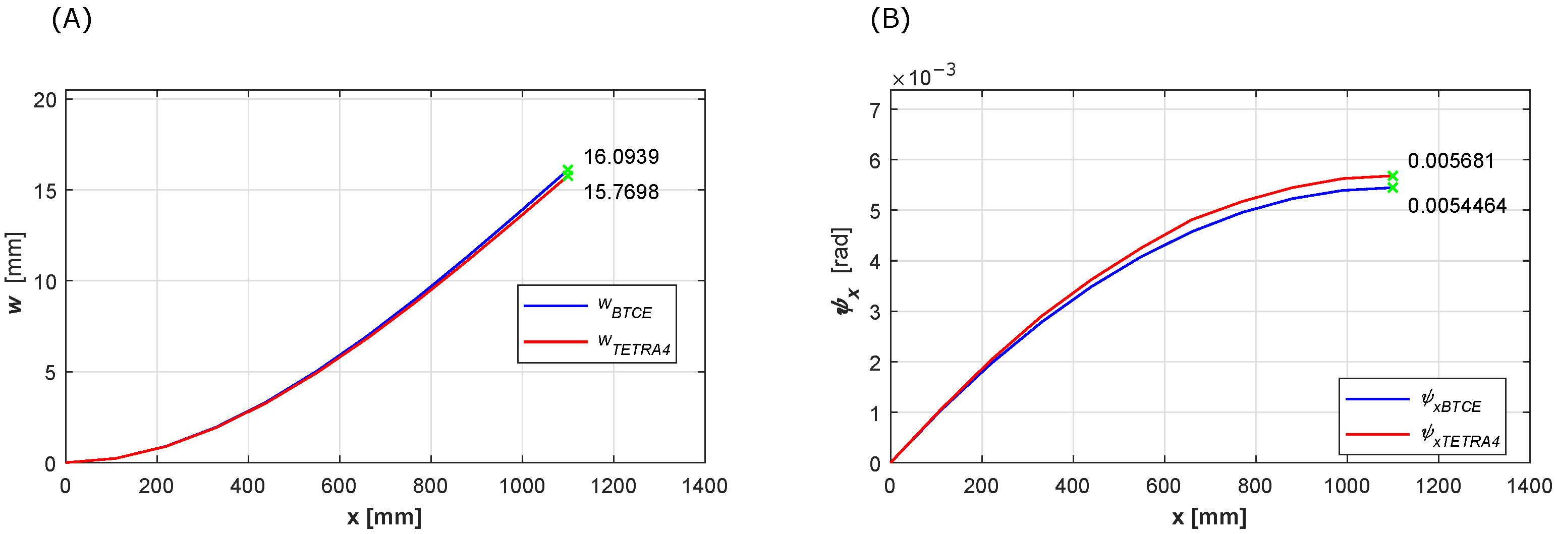
The results of the linear static analysis for the load cases presented in Table 7 obtained for the BTCE model here derived have been compared with the numerical results of a TETRA4 FE model with the same load configuration for Test Case 1. Vertical deflection and torsion angle results have been collected and represented in Figure 7, Figure 8 and 
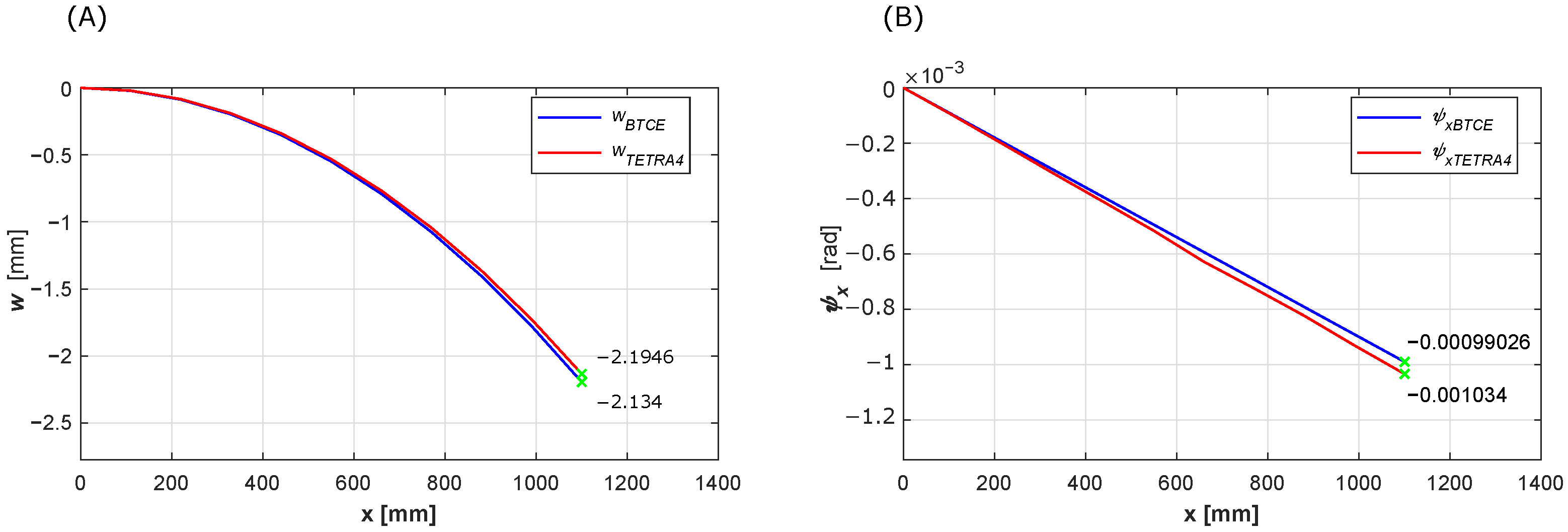
Figure 9. The results reveal a good correlation between the two numerical model considered for each load case, showing the capability of the BTCE to correctly represent the bending-torsion coupling effect given by the stiffeners in presence of a static load.
The values of the deformations at the free end of the beam are reported in Table 8, the relative difference is computed with Equation (22) considering the result of the TETRA4 model as reference value. The relative difference is computed also for each node along the beam and the mean value is reported in the last column of Table 8. In the same table also the results of the deformation at the free end of the beam for the uncoupled case ( C 12 = 0 ) are reported, the reference values for the comparison are computed with the PVW. The comparison shows a difference lower than 5 % for the load cases considered with a slightly higher value for the torsion angle computed for load case 3. This could be caused by an overestimation of the torsional stiffness C 11 computed with Equation (1). The approximation introduced when the cross section of the beam is reduced to its mid thickness line can affect the final stiffness of the beam. The results for the uncoupled configuration are in line with the analytical formulation.

5.2. Modal Analysis Results

The results of the modal analysis for Test Case 1 obtained with the procedure described in the previous section have been compared with experimental, numerical and analytical results. The frequencies computed considering the bending and torsion uncoupled ( C 12 = 0 ) are reported in Table 9 while the frequencies obtained with the TETRA4 FE model are reported in 
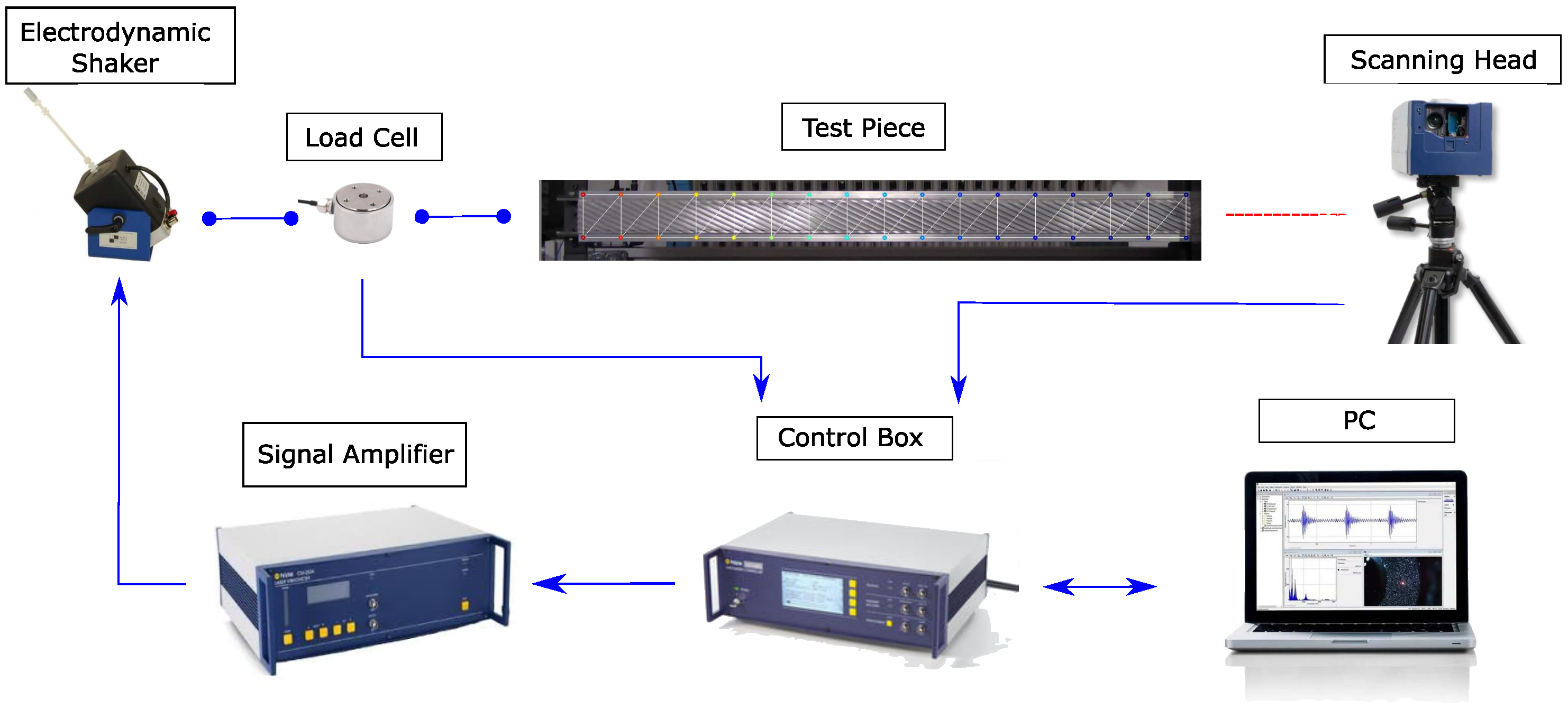
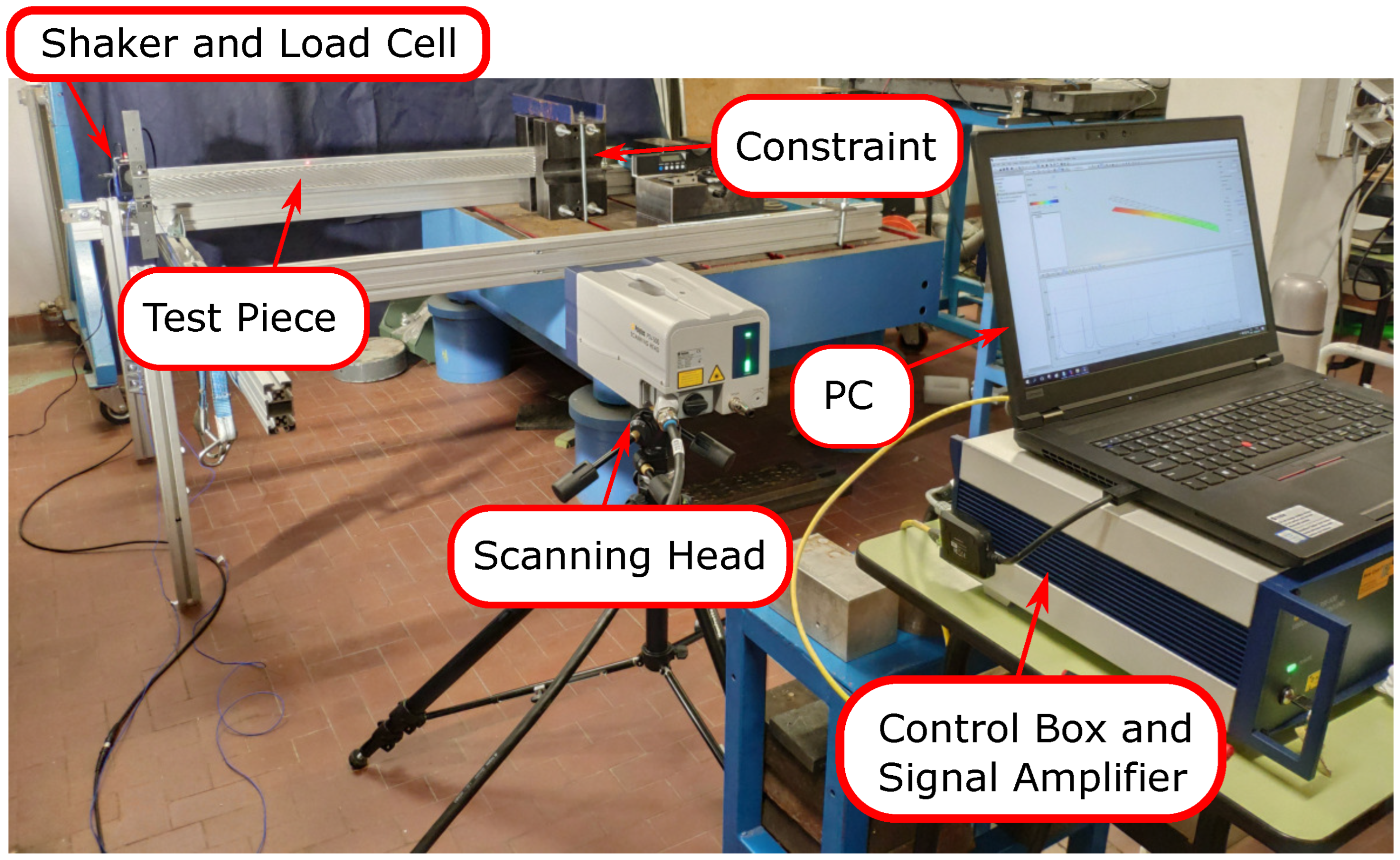
Table 10. The experimental results have been acquired by Patuelli et al. [18] with a laser Doppler vibrometer according to the procedure described in [35] and reported in Table 11 for a comparison. The second and fourth mode do not present experimental frequency value or mode shape. Due to the nature of the acquisition, the experimental modal analysis did not include the in-plane modes since the focus was on the bending-torsion coupling effect which does not affects the neglected modes.
The comparison with the analytical frequencies confirmed the consistency of the model for the uncoupled case with a negligible relative difference. Moreover, the comparison with numerical results revealed that there is good agreement between the present theory and the TETRA FE model, with relative error lower than 5 % for most of the natural frequencies computed. The natural frequency of the 6th mode present an higher relative difference of 9.29 % .
The correlation with experimental results is generally good, with a relative error around 5 % or lower for the 1st and the 5th mode, but with a considerably higher difference for the 3rd and the 6th mode. There are mainly two reason for the difference in natural frequencies values. As already stated before, the approximation introduced when the cross section of the beam is reduced to its mid thickness line affect the stiffness coefficients, but also the inertia properties of the beam. Moreover, the experimental results are affected by a constraint condition impossible to replicate for the beam element. The beam was clamped between two steel blocks applying pressure on the upper and lower face of the first 100 mm of the beam. With this configuration, the first section of the beam was not fully constrained which is the condition applied to the BTCE section when imposing all the degrees of freedom equals to zero for the first node.
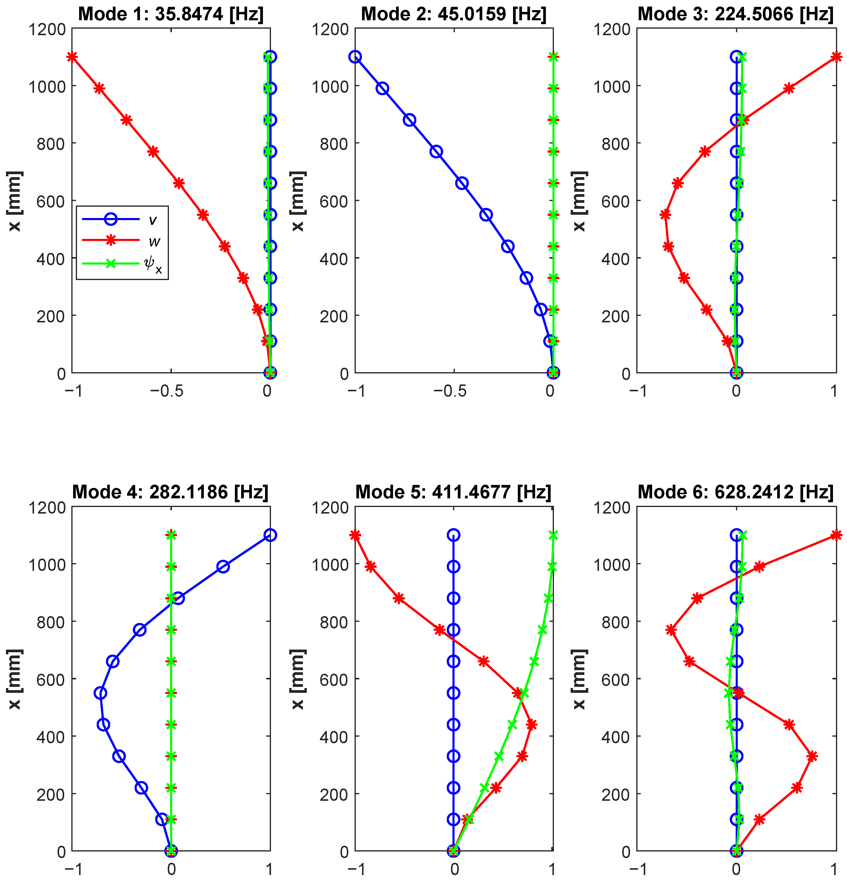
The eigenvectors solution of Equation (24) for the BTCE model are graphically represented in Figure 10. Only the three components of the eigenvectors involved in the modes investigated are represented, the in-plane component v, the out-of-plane component w, and the torsional component ψ x . The eigenvectors components have been normalized with respect to the maximum value present among all the degrees of freedom for a given mode.
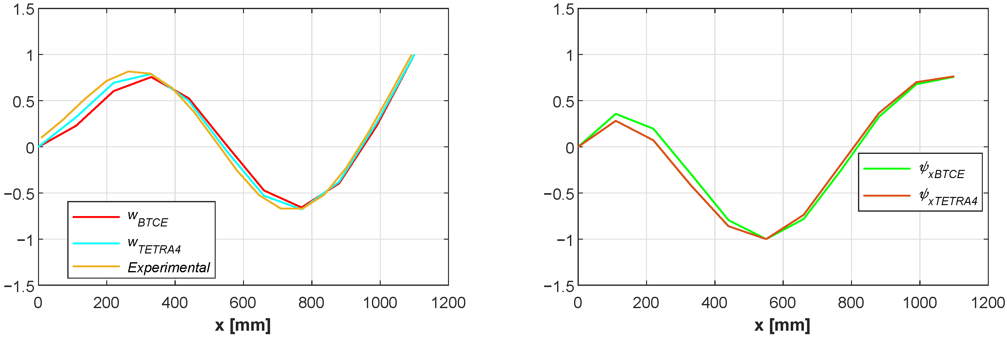
The eigenvectors depicted in Figure 10 highlight the coupling effect for the 1st, 3rd, 5th and 6th mode where the 1st, 3rd and 6th mode are mainly bending modes with respect to the y-axis and the 5th is mainly a torsional mode around x-axis. It is worth noting that the 2nd and 4th mode which are the bending modes with respect to the z-axis are correctly not influenced by the coupling term C 12 
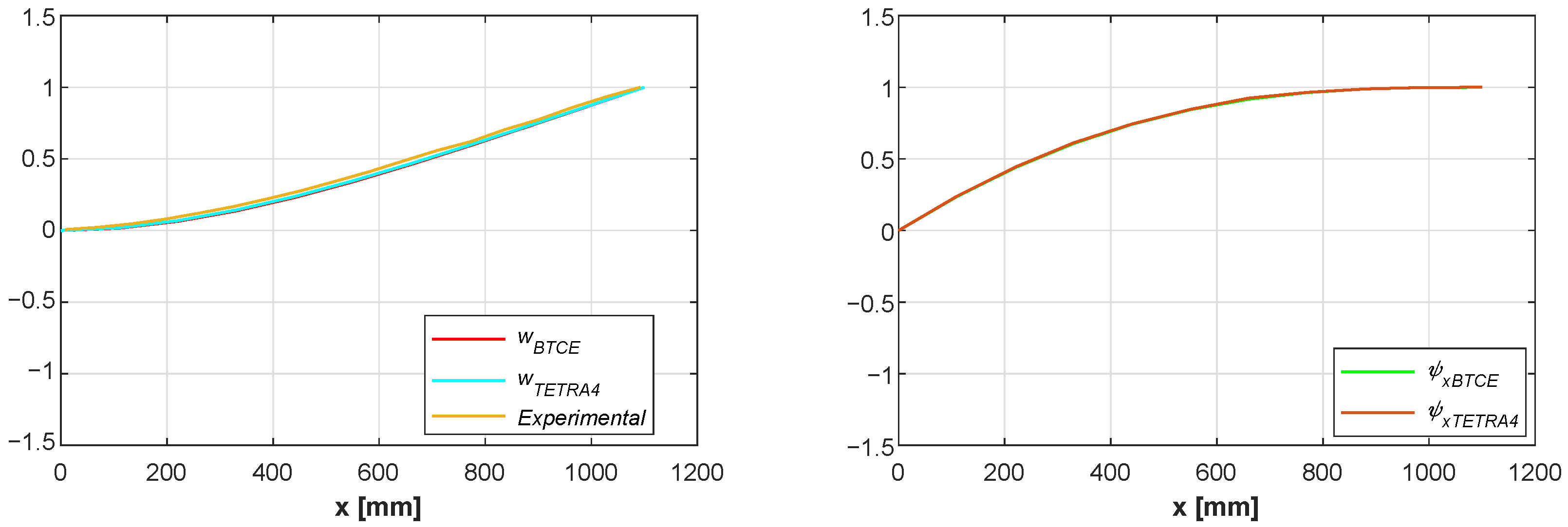
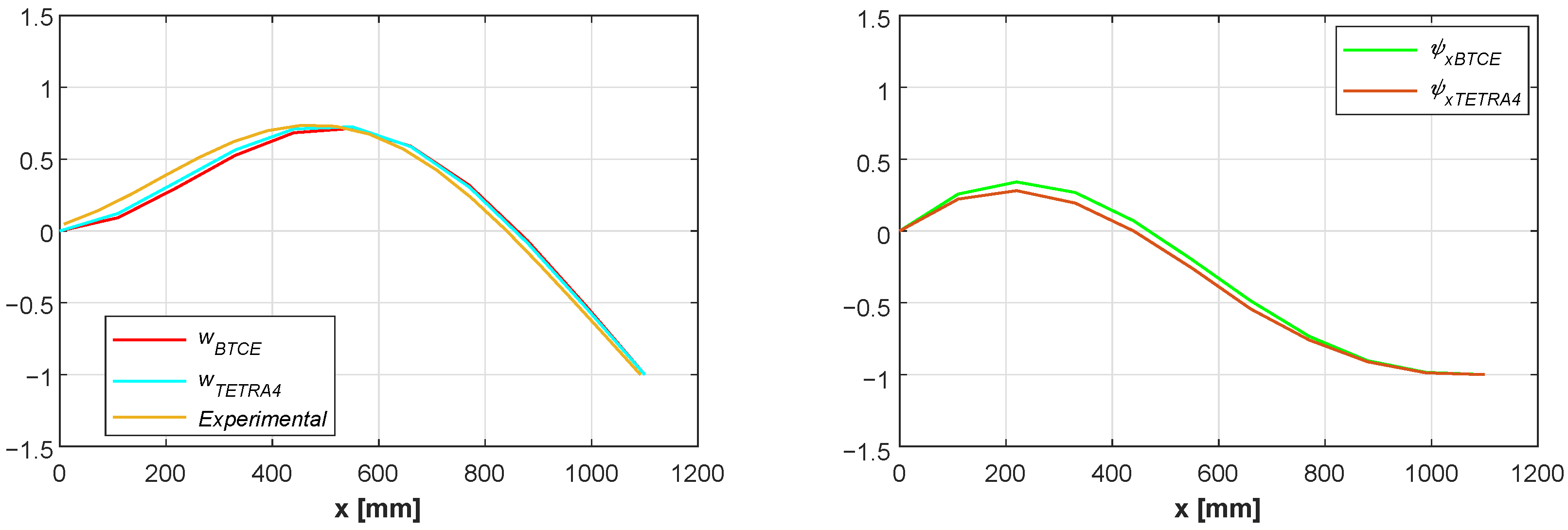
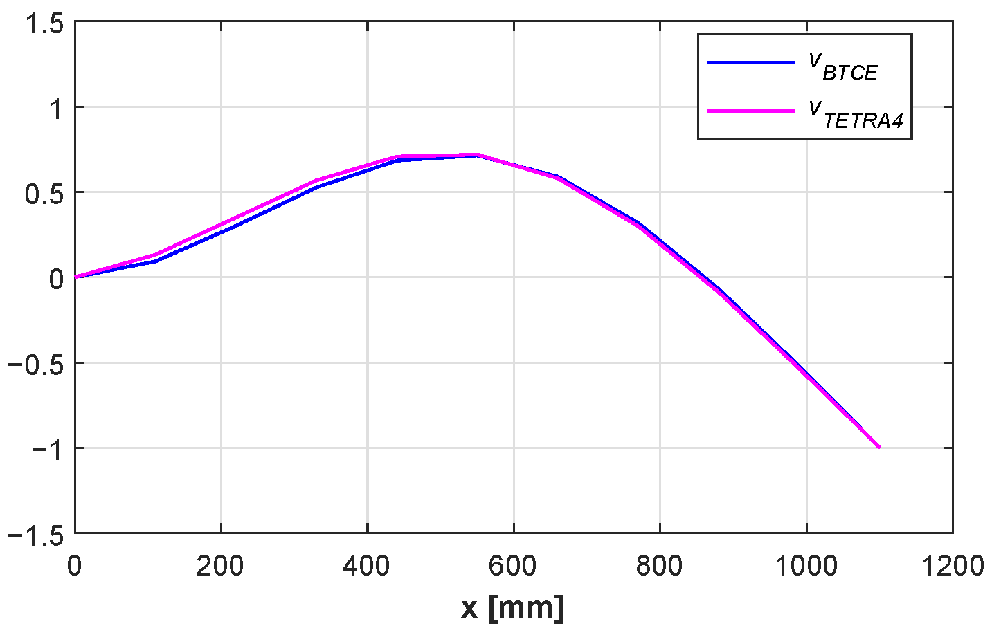
and result uncoupled. Similar observation can be made for the comparison reported in Figure 12, Figure 13, Figure 14, Figure 15, Figure 16 and Figure 17, where the mode shapes and the coupling effects are in accordance with the results obtained for the TETRA4 model. Furthermore, the mode shapes are in good agreement with experimental results for the z component of the eigeinvectors reported in [18].
A convergence study on the computed natural frequencies has been performed considering a number of elements varying from 3 to 50. The results are represented in Figure 11 in terms of natural frequency normalized with respect to the convergence value. It is possible to observe that the first three natural frequencies converge rapidly with the increase in the number of elements and their curves result coincident in Figure 11, while the fourth, fifth and sixth mode require more elements to converge. However, the natural frequency computed for Mode 6 with 10 elements is only 0.026 % greater than the convergence value.
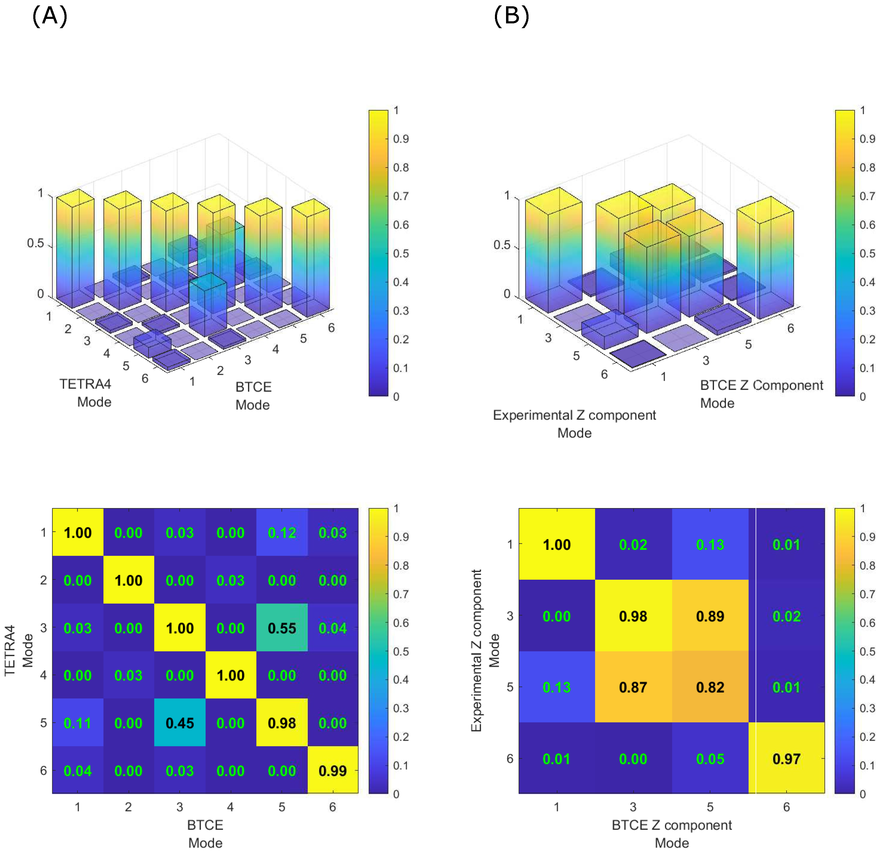
The MAC matrices computed for the mode shape comparisons are reported in Figure 18. The BTCE model showed an excellent accordance with the TETRA4 model as reported in Figure 18A. The results revealed a similarity between the 3rd and the 5th mode, which was expected because the torsional mode (Mode 5) is coupled with bending through the coupling term C 12 = K in the stiffness matrix. This coupling effect generate a component along z-axis for the 5th mode which is similar to the same component for the second bending mode (Mode 3) as can be observed in Figure 14 and Figure 16. The same coupling effects are observable in the comparison with experimental results (Figure 18B), this is testified by the off diagonal values related to the 3rd and the 5th mode. The similarity is higher because in this case only the component of the eigenvectors along z-axis is considered. The relatively low similarity between the 5th BTCE mode and the corresponding experimental mode is probably related to the reduced number of acquisition points along the beam axis during the physical test.
The results of the modal analysis performed on the BTCE model of the NREL 5MW HAWAT blade described in [19] are reported in Table 12. The results have been compared with the natural frequency obtained with Rayleigh theory, with Timoshenko theory and with Bernoulli theory reported in [32]. The values computed with the BTCE model have been compared also with the results obtained with two software developed by NREL [32], B-Modes and FAST, with the results obtained by Jeong et al. [34] using BEM-ABAQUS commercial software and with the results obtained by Li et al. [33] where a geometrically exact beam theory was used.
The BTCE model showed great accordance with other beam theories and commercial software results, with a relative difference below 5% for the computed natural frequencies. The error is considerably higher when the BTCE model is compared to the Bernoulli theory, however the natural frequency computed with the Bernoulli theory for the third and the fifth frequencies are not in accordance with the other theories or commercial solvers.
The results of the modal analysis performed on the CAS graphite/epoxy box beam are reported in Table 13. The natural frequency have been compared with numerical results from [20] and experimental data reported in [21] computing the relative differences with Equation (22).
The results are in good agreement with numerical and experimental results with a relative difference with the BTCE model natural frequencies mostly lower than 7% for both layups. Minor discrepancies can be observed for the for the first horizontal bending mode frequency where the relative difference with the experimental result is equal to 13.81%

6. Conclusions

The derivation of a beam finite element for structures with bending-torsion coupling was presented in this work. The shape functions have been derived consistently with the equilibrium and kinematics equations while the stiffness and mass matrix have been obtained through the Galerkin’s method. The matrices derived have been used to create a BTCE model of a beam structure and solve the linear static and eigenvalue problems.
The present model was validated for the static case through the simulation of an aluminum beam with stiffened panels and cantilever configuration for three different load configurations applied at the free end of the beam. The oriented stiffeners consented to achieve an appreciable bending-torsion coupling effect which was correctly represented by the results of the static and modal analysis.
The results obtained from the static analysis have been compared with the results of a TETRA4 FE model in the same configuration. The relative differences between the maximum value of displacement and torsion angle computed for the BTCE and the TETRA4 model is below 5% for most of the load cases considered. The relative difference between the two models along the length of the beam is mostly lower than 5%. Minor discrepancies are induced by the approximation introduced when the cross section of the beam is reduced to its mid thickness line which affect the stiffness coefficients.
The beam element has been validated also for the dynamic case with a modal analysis in the cantilever configuration. The results obtained have been compared with experimental results and with a TETRA4 FE model numerical results showing a relative error mostly lower than 5 % in terms of natural frequency value for the numerical comparison and higher values for the experimental comparison, up to 10 % in the worst case. These discrepancies can be explained considering that the beam cross section was reduced to its mid thickness line for the BTCE model. This introduced approximations that can affects also the inertia properties of the beam. Moreover the constraints applied during the experimental tests with a root section not perfectly constrained, could not be replicated with the beam element where the same section is considered fixed.
The similarity between the mode shape obtained with the present theory have been compared with the TETRA4 FE model and experimental mode shapes with the modal assurance criterion. The computed MAC matrices showed great accordance between the sets of mode shape compared, with minor discrepancies with the experimental results comparison connected to a relatively low number of scanning points during the experimental tests.
The finite element has been tested for the modal analysis of a NREL 5MW HAWT blade with variable cross-sectional properties and of a CAS graphite/epoxy cantilever box beam with different layups. The natural frequencies have been compared with numerical and experimental results showing good accordance with the BTCE model and confirming the compatibility of the new finite element with these classes of structures.
The coupled beam finite element is validated with numerical and experimental evidence for different structures, where the coupling effect is given by oriented stiffeners or oriented composite material. Moreover, the model is consistent with kinematics and equilibrium equation and its application is not limited to box-section beams. The beam element presented in this research can be extended for non-linear static and dynamic analysis and used to solve aeroelastic problems with fluid-structure interactions or for aerodynamic tailoring purposes.

Author Contributions

C.P.: Methodology, Data curation, Formal analysis, Validation, Visualization, Writing—original draft. E.C.: Supervision, Conceptualization, Writing—review/editing. G.F.: Supervision, Conceptualization, Writing—review/editing. All authors have read and agreed to the published version of the manuscript.

Funding

This research received no external funding.

Data Availability Statement

The data presented in this study are available on request from the corresponding author.

Conflicts of Interest

The authors declare no conflict of interest.

Appendix A

Appendix A.1. Boundary Conditions

The integration by parts of Equations (16) results in the following equations:
0 L { N v } ρ A 2 v ( e ) 2 t d x + 0 L { N v } E I z 2 v ( e ) x 2 d x = 0 L { N v } f v d x { N v } E I z x 2 v ( e ) x 2 | 0 L + { N v } E I z 2 v ( e ) x 2 | 0 L
0 L { N w } ρ A 2 w ( e ) t 2 d x + 0 L { N w } E I y 2 w ( e ) x 2 d x 0 L { N w } K ψ ( e ) x d x = 0 L { N w } f w d x { N w } E I y x 2 w ( e ) x 2 | 0 L + { N w } K 2 ψ ( e ) x 2 | 0 L + { N w } E I y 2 w ( e ) x 2 | 0 L { N w } K ψ ( e ) x | 0 L
0 L { N ψ } ρ A 2 ψ ( e ) 2 t d x + 0 L { N ψ } G J t ψ ( e ) x d x 0 L { N ψ } K 2 w ( e ) x 2 d x = 0 L { N ψ } f ψ d x + { N ψ } G J t ψ ( e ) x | 0 L { N ψ } K 2 w ( e ) x 2 | 0 L
The right part of Equations (A1a–c) can be rewritten to obtain the element nodal forces and moments.
0 L { N v } f v d x + N v 1 E I z x 2 v ( e ) x 2 | 0 L N v 2 E I z x 2 v ( e ) x 2 | 0 L N v 3 E I z x 2 v ( e ) x 2 | 0 L N v 4 E I z x 2 v ( e ) x 2 | 0 L + N v 1 E I z 2 v ( e ) x 2 | 0 L N v 2 E I z 2 v ( e ) x 2 | 0 L N v 3 E I z 2 v ( e ) x 2 | 0 L N v 4 E I z 2 v ( e ) x 2 | 0 L
0 L { N w } f w d x + N w 1 E I y x 2 w ( e ) x 2 + K 2 ψ ( e ) x 2 | 0 L N w 2 E I y x 2 w ( e ) x 2 + K 2 ψ ( e ) x 2 | 0 L N w 3 E I y x 2 w ( e ) x 2 + K 2 ψ ( e ) x 2 | 0 L N w 4 E I y x 2 w ( e ) x 2 + K 2 ψ ( e ) x 2 | 0 L + N w 1 E I y 2 w ( e ) x 2 K ψ ( e ) x | 0 L N w 2 E I y 2 w ( e ) x 2 K ψ ( e ) x | 0 L N w 3 E I y 2 w ( e ) x 2 K ψ ( e ) x | 0 L N w 4 E I y 2 w ( e ) x 2 K ψ ( e ) x | 0 L
0 L { N ψ } f ψ d x + N ψ 1 G J t ψ ( e ) x K 2 w ( e ) x 2 | 0 L N ψ 2 G J t ψ ( e ) x K 2 w ( e ) x 2 | 0 L N ψ 3 G J t ψ ( e ) x K 2 w ( e ) x 2 | 0 L N ψ 4 G J t ψ ( e ) x K 2 w ( e ) x 2 | 0 L N ψ 5 G J t ψ ( e ) x K 2 w ( e ) x 2 | 0 L N ψ 6 G J t ψ ( e ) x K 2 w ( e ) x 2 | 0 L
Knowing that:
E I z x 2 v ( e ) x 2 = T y E I z 2 v ( e ) x 2 = M z E I y x 2 w ( e ) x 2 + K 2 ψ ( e ) x 2 = T z E I y 2 w ( e ) x 2 + K ψ ( e ) x = M y G J t ψ ( e ) x K 2 w ( e ) x 2 = M x
and that the shape functions and their derivatives assumes the following values for the first node ( x = 0 ) and the second node ( x = L ) of the element:
N v 1 ( 0 ) = 1 , N v 1 ( L ) = 0 , N v 1 ( 0 ) = 0 , N v 1 ( L ) = 0 N v 2 ( 0 ) = 0 , N v 2 ( L ) = 0 , N v 2 ( 0 ) = 1 , N v 2 ( L ) = 0 N v 3 ( 0 ) = 0 , N v 3 ( L ) = 1 , N v 3 ( 0 ) = 0 , N v 3 ( L ) = 0 N v 4 ( 0 ) = 0 , N v 4 ( L ) = 0 , N v 4 ( 0 ) = 0 , N v 4 ( L ) = 1
N w 1 ( 0 ) = 1 , N w 1 ( L ) = 0 , N w 1 ( 0 ) = 0 , N w 1 ( L ) = 0 N w 2 ( 0 ) = 0 , N w 2 ( L ) = 0 , N w 2 ( 0 ) = 1 , N w 2 ( L ) = 0 N w 3 ( 0 ) = 0 , N w 3 ( L ) = 1 , N w 3 ( 0 ) = 0 , N w 3 ( L ) = 0 N w 4 ( 0 ) = 0 , N w 4 ( L ) = 0 , N w 4 ( 0 ) = 0 , N w 4 ( L ) = 1
N ψ 1 ( 0 ) = 1 , N ψ 1 ( L ) = 0 N ψ 2 ( 0 ) = 0 , N ψ 2 ( L ) = 0 N ψ 3 ( 0 ) = 0 , N ψ 3 ( L ) = 0 N ψ 4 ( 0 ) = 0 , N ψ 4 ( L ) = 1 N ψ 5 ( 0 ) = 0 , N ψ 5 ( L ) = 0 N ψ 6 ( 0 ) = 0 , N ψ 6 ( L ) = 0
Equation (17) are obtained.

Appendix A.2. Stiffness and Mass Matrices

[ K v ] = 0 L E I z { N v } { N v } d x = E I z L 3 12 6 L 12 6 L 4 L 2 6 L 2 L 2 12 6 L 4 L 2
[ K w ] = 0 L E I y { N w } { N w } d x = E I y L 3 12 6 L 12 6 L 4 L 2 6 L 2 L 2 12 6 L 4 L 2
[ K ψ ] = 0 L G J t { N ψ } { N ψ } d x = G J t L 0 0 G J t L 0 0 12 K 2 G J t L 3 6 K 2 G J t L 2 0 12 K 2 G J t L 3 6 K 2 G J t L 2 3 K 2 G J t L 0 6 K 2 G J t L 2 3 K 2 G J t L G J t L 0 0 12 K 2 G J t L 3 6 K 2 G J t L 2 3 K 2 G J t L
[ K w ψ ] = 0 L K { N w } { N ψ } d x = 0 12 K G J t L 3 6 K G J t L 2 0 12 K G J t L 3 6 K G J t L 2 1 L 6 K G J t L 2 3 K G J t L 1 L 6 K G J t L 2 3 K G J t L 0 12 K G J t L 3 6 K G J t L 2 0 12 K G J t L 3 6 K G J t L 2 1 L 6 K G J t L 2 3 K G J t L 1 L 6 K G J t L 2 3 K G J t L
[ K ψ w ] = 0 L K { N ψ } { N w } d x = 0 1 L 0 1 L 12 K 2 G J t L 3 6 K 2 G J t L 2 12 K 2 G J t L 3 6 K 2 G J t L 2 6 K 2 G J t L 2 3 K 2 G J t L 6 K 2 G J t L 2 3 K 2 G J t L 0 1 L 0 1 L 12 K 2 G J t L 3 6 K 2 G J t L 2 12 K 2 G J t L 3 6 K 2 G J t L 2 6 K 2 G J t L 2 3 K 2 G J t L 6 K 2 G J t L 2 3 K 2 G J t L
[ M v ] = 0 L ρ A { N v } { N v } d x = ρ A L 210 78 11 L 27 13 L 2 2 L 2 13 L 2 3 L 2 2 78 11 L 2 L 2
[ M w ] = 0 L ρ A { N w } { N w } d x = ρ A L 210 78 11 L 27 13 L 2 2 L 2 13 L 2 3 L 2 2 78 11 L 2 L 2
[ M ψ ] = 0 L ρ A { N ψ } { N ψ } d x = ρ I p L 3 K 2 G J t K L 4 G J t L 6 K 2 G J t K L 4 G J t 6 K 2 5 G J t 2 L 3 K 2 5 G J t 2 K 2 G J t 6 K 2 5 G J t 2 L 3 K 2 5 G J t 2 3 K 2 L 10 G J t 2 K L 4 G J t 3 K 2 5 G J t 2 3 K 2 L 10 G J t 2 L 3 K 2 G J t K L 4 G J t 6 K 2 5 G J t 2 L 3 K 2 5 G J t 2 3 K 2 L 10 G J t 2
It is now possible to define the array q which include all the nodal degree of freedom for a two node element as:
q = { v 1 , w 1 , ψ 1 , θ 1 y , θ 1 z , v 2 , w 2 , ψ 2 , θ 2 y , θ 2 z }
The finite element global stiffness matrix [K] and mass matrix [M] can be obtained combining matrices (A7) to (A14) with the sum of the members involving the same degrees of freedom.
[ K ] = 12 E I z L 3 0 0 0 6 E I z L 2 12 E I z L 3 0 0 0 6 E I z L 2 K 1 0 K 2 0 0 K 1 0 K 2 0 G J t L K L 0 0 0 G J t L K L 0 K 3 0 0 K 2 K L K 4 0 4 E I z L 6 E I z L 2 0 0 0 2 E I z L 12 E I z L 3 0 0 0 6 E I z L 2 K 1 0 K 2 0 G J t L K L 0 K 3 0 4 E I z L
with
c c K 1 = 12 ( E I y G J t K 2 ) G J t L 3 K 2 = 6 ( K 2 E I y G J t ) G J t L 2 K 3 = 4 E I y G J t 3 K 2 G J t L K 4 = 2 E I y G J t 3 K 2 G J t L
[ M ] = 13 A L ρ 35 0 0 0 11 A L 2 ρ 210 9 A L ρ 70 0 0 0 13 A L 2 ρ 420 M 1 I p K ρ 2 G J t M 2 0 0 M 3 I p K ρ 2 G J t M 4 0 I p L ρ 3 I p K L ρ 4 G J t 0 0 I p K ρ 2 G J t I p L ρ 6 I p K L ρ 4 G J t 0 M 5 0 0 M 4 I p K L ρ 4 G J t M 6 0 A L 3 ρ 105 13 A L 2 ρ 420 0 0 0 A L 3 ρ 140 13 A L ρ 35 0 0 0 11 A L 2 ρ 210 M 1 I p K ρ 2 G J t M 2 0 I p L ρ 3 I p K L ρ 4 G J t 0 M 5 0 A L 3 ρ 105
with
M 1 = 6 I p K 2 ρ 5 G J t 2 L + 13 A L ρ 35 M 2 = 3 I p K 2 ρ 5 G J t 2 11 A L 2 ρ 210 M 3 = 6 I p K 2 ρ 5 G J t 2 L + 9 A L ρ 70 M 4 = 3 I p K 2 ρ 5 G J t 2 + 13 A L 2 ρ 420 M 5 = 3 I p K 2 L ρ 10 G J t 2 + A L 3 ρ 105 M 6 = 3 I p K 2 L ρ 10 G J t 2 A L 3 ρ 140
It is worth noting that if the configuration is uncoupled and K is equal to 0, the matrices [K] and [M] are the standard Hermitian beam element uncoupled matrices.

References

  1. Hansen, M.; Sørensen, J.; Voutsinas, S.; Sørensen, N.; Madsen, H. State of the art in wind turbine aerodynamics and aeroelasticity. Prog. Aerosp. Sci. 2006, 42, 285–330. [Google Scholar] [CrossRef]
  2. Hansen, M. Aeroelastic instability problems for wind turbines. Wind Energy 2007, 10, 551–577. [Google Scholar] [CrossRef]
  3. Patil, M.; Hodges, D. Flight Dynamics of Highly Flexible Flying Wings. J. Aircr. 2006, 43, 1790–1799. [Google Scholar] [CrossRef]
  4. Afonso, F.; Lobo do Vale, J.; Oliveira, É.; Lau, F.; Suleman, A. A review on non-linear aeroelasticity of high aspect-ratio wings. Prog. Aerosp. Sci. 2017, 89, 40–57. [Google Scholar] [CrossRef]
  5. Cestino, E.; Frulla, G.; Spina, M.; Catelani, D.; Linari, M. Numerical simulation and experimental validation of slender wings flutter behaviour. Proc. Inst. Mech. Eng. Part G J. Aerosp. Eng. 2019, 233, 5913–5928. [Google Scholar] [CrossRef]
  6. Shirk, M.; Hertz, T.; Weisshaar, T. Aeroelastic tailoring—Theory, practice, and promise. J. Aircr. 1986, 23, 6–18. [Google Scholar] [CrossRef]
  7. Kameyama, M.; Fukunaga, H. Optimum design of composite plate wings for aeroelastic characteristics using lamination parameters. Comput. Struct. 2007, 85, 213–224. [Google Scholar] [CrossRef]
  8. Weisshaar, T. Aeroelastic Tailoring of Forward Swept Composite Wings. J. Aircr. 1981, 18, 669–676. [Google Scholar] [CrossRef]
  9. Dokumaci, E. An exact solution for coupled bending and torsion vibrations of uniform beams having single cross-sectional symmetry. J. Sound Vib. 1987, 119, 443–449. [Google Scholar] [CrossRef]
  10. Hashemi, S.; Richard, M. A Dynamic Finite Element (DFE) method for free vibrations of bending-torsion coupled beams. Aerosp. Sci. Technol. 2000, 4, 41–55. [Google Scholar] [CrossRef]
  11. Mohri, F.; Ed-dinari, A.; Damil, N.; Potier-Ferry, M. A beam finite element for non-linear analyses of thin-walled elements. Thin-Walled Struct. 2008, 46, 981–990. [Google Scholar] [CrossRef]
  12. Cestino, E.; Frulla, G.; Marzocca, P. A Reduced Order Model for the Aeroelastic Analysis of Flexible Wings. SAE Int. J. Aerosp. 2013, 6, 447–458. [Google Scholar] [CrossRef]
  13. Babuska, P.; Wiebe, R.; Motley, M.R. A beam finite element for analysis of composite beams with the inclusion of bend-twist coupling. Compos. Struct. 2018, 189, 707–717. [Google Scholar] [CrossRef]
  14. Nam, V.; Vinh, P.; Chinh, N.; Thom, D.; Hong, T. A New Beam Model for Simulation of the Mechanical Behaviour of Variable Thickness Functionally Graded Material Beams Based on Modified First Order Shear Deformation Theory. Materials 2019, 12, 404. [Google Scholar] [CrossRef]
  15. Dung, N.; Tho, N.; Ha, N.; Hieu, V. On the Finite Element Model of Rotating Functionally Graded Graphene Beams Resting on Elastic Foundation. Math. Probl. Eng. 2021, 2021, 1586388. [Google Scholar] [CrossRef]
  16. Banerjee, J.; Su, H. Free Transverse and Lateral Vibration of Beams with Torsional Coupling. J. Aerosp. Eng. 2006, 19, 13–20. [Google Scholar] [CrossRef]
  17. Cestino, E.; Frulla, G. Analysis of slender thin-walled anisotropic box-beams including local stiffness and coupling effects. Aircr. Eng. Aerosp. Technol. Int. J. 2014, 86, 345–355. [Google Scholar] [CrossRef]
  18. Patuelli, C.; Polla, A.; Cestino, E.; Frulla, G. Experimental and Numerical Dynamic Behavior of Bending-Torsion Coupled Box-Beam. J. Vib. Eng. Technol. 2022. [Google Scholar] [CrossRef]
  19. Jonkman, J.; Butterfield, S.; Musial, W.; Scott, G. Definition of a 5 MW Reference Wind Turbine for Offshore System Development; National Renewable Energy Laboratory (NREL): Golden, CO, USA, 2009. [CrossRef]
  20. Armanios, E.; Badir, A. Free vibration analysis of anisotropic thin-walled closed-section beams. Aiaa J. 1995, 33, 1905–1910. [Google Scholar] [CrossRef]
  21. Chandra, R.; Chopra, I. Experimental-theoretical investigation of the vibration characteristics of rotating composite box beams. J. Aircr. 1992, 29, 657–664. [Google Scholar] [CrossRef]
  22. Nayfeh, A.; Pai, P. Linear and Nonlinear Structural Mechanics; John Wiley & Sons: Hoboken, NJ, USA, 2004. [Google Scholar] [CrossRef]
  23. Hodges, D.; Dowell, E. Nonlinear Equations of Motion for the Elastic Bending and Torsion of Twisted Nonuniform Rotor Blades. No. A-5711. 1974. Available online: https://ntrs.nasa.gov/citations/19750005242 (accessed on 29 November 2022).
  24. Silva, M.; Glynn, C. Nonlinear Flexural-Flexural-Torsional Dynamics of Inextensional Beams. I. Equations of Motion. J. Struct. Mech. 1978, 6, 437–448. [Google Scholar] [CrossRef]
  25. Danzi, F.; Cestino, E.; Frulla, G.; Gibert, J. Equivalent plate model of curvilinear stiffened panels. In Proceedings of the M2D2017, Albufeira, Portugal, 11–15 June 2017; pp. 553–568, ISBN 978-989-98832-7-7. [Google Scholar]
  26. Kramer, M.; Liu, Z.; Young, Y.L. Free vibration of cantilevered composite plates in air and in water. Compos. Struct. 2013, 95, 254–263. [Google Scholar] [CrossRef]
  27. Weisshaar, T.; Foist, B. Vibration tailoring of advanced composite lifting surfaces. J. Aircr. 1985, 22, 141–147. [Google Scholar] [CrossRef]
  28. Hodges, D.; Pierce, G. Introduction to Structural Dynamics and Aeroelasticity; Cambridge University Press: Cambridge, UK, 2011. [Google Scholar] [CrossRef]
  29. Nemeth, M. NASA/TP-20—A Treatise on Equivalent-Plate Stiffnesses for Stiffened Laminated-Composite Plates and Plate-like Lattices; Technical Report; NASA Langley Research Center: Hampton, VA, USA, 2011.
  30. Pastor, M.; Binda, M.; Harčarik, T. Modal Assurance Criterion. Procedia Eng. 2012, 48, 543–548. [Google Scholar] [CrossRef]
  31. Ewins, D. Modal Testing, Theory, Practice and Application, 2nd ed.; Research Studies Press Ltd.: Baldock/Hertfordshire, UK, 2000. [Google Scholar]
  32. ALGOLFAT, A.; Wang, W.; Albarbar, A. Dynamic Responses Analysis of A 5MW NREL Wind Turbine Blade Under Flap-Wise and Edge-Wise Vibrations. J. Dyn. Monit. Diagn. 2022, 1, 208–222. [Google Scholar] [CrossRef]
  33. Li, Z.W.; Wen, B.; Dong, X.J.; Peng, Z.; Qu, Y.; Zhang, W. Aerodynamic and aeroelastic characteristics of flexible wind turbine blades under periodic unsteady inflows. J. Wind Eng. Ind. Aerodyn. 2019, 2020, 105057. [Google Scholar] [CrossRef]
  34. Jeong, M.S.; Cha, M.C.; Kim, S.W.; Lee, I.; Kim, T. Effects of Torsional Degree of Freedom, Geometric Nonlinearity, and Gravity on Aeroelastic Behavior of Large-Scale Horizontal-Axis Wind Turbine Blades under Varying Wind Speed Conditions. J. Renew. Sustain. Energy 2014, 6, 023126. [Google Scholar] [CrossRef]
  35. Praticò, L.; Galos, J.; Cestino, E.; Frulla, G.; Marzocca, P. Experimental and numerical vibration analysis of plates with curvilinear sub-stiffeners. Eng. Struct. 2019, 209, 109956. [Google Scholar] [CrossRef]
Figure 1. Beam Element reference system with dimensions, nodal degrees of freedom and resultants.
Aerospace 10 00142 g001
Figure 2. Aluminum Beam dimensions with mid-thickness line of the section, from [18] used under Creative Commons CC-BY license.
Aerospace 10 00142 g002
Figure 3. (A) TETRA4 FE model, (B) Detail of the MPC for free end load application, (C) Detail of the constrained nodes.
Aerospace 10 00142 g003
Figure 4. Cross-Sectional Stiffness properties of NREL 5 MW HAWT blade [19] (Test Case 2).
Aerospace 10 00142 g004
Figure 5. Experimental Setup Scheme, from [18] used under Creative Commons CC-BY license.
Aerospace 10 00142 g005
Figure 6. Experimental Setup for Test Case 1.
Aerospace 10 00142 g006
Figure 7. Load Case 1 Results Comparison (Test Case 1), (A) Deflection along z-axis, (B) Torsion Angle.
Aerospace 10 00142 g007
Figure 8. Load Case 2 Results Comparison (Test Case 1), (A) Deflection along z-axis, (B) Torsion Angle.
Aerospace 10 00142 g008
Figure 9. Load Case 3 Results Comparison (Test Case 1), (A) Deflection along z-axis, (B) Torsion Angle.
Aerospace 10 00142 g009
Figure 10. BTCE Modal Analysis Results with eigenvectors components along z and y-axis and rotational component along x-axis (Test Case 1).
Aerospace 10 00142 g010
Figure 11. BTCE Modal Analysis Results convergence study. (Test Case 1).
Aerospace 10 00142 g011
Figure 12. First Mode Shape Comparison between BTCE, TETRA4 and Experimental [18] results (Test Case 1).
Aerospace 10 00142 g012
Figure 13. Second Mode Shape Comparison between BTCE and TETRA4 results (Test Case 1).
Aerospace 10 00142 g013
Figure 14. Third Mode Shape Comparison between BTCE, TETRA4 and Experimental [18] results (Test Case 1).
Aerospace 10 00142 g014
Figure 15. Fourth Mode Shape Comparison between BTCE and TETRA4 results (Test Case 1).
Aerospace 10 00142 g015
Figure 16. Fifth Mode Shape Comparison between BTCE, TETRA4 and Experimental [18] results (Test Case 1).
Aerospace 10 00142 g016
Figure 17. Sixth Mode Shape Comparison between BTCE, TETRA4 and Experimental [18] results (Test Case 1).
Aerospace 10 00142 g017
Figure 18. (A) MAC matrix for TETRA4-BTCE mode shapes comparison; (B) MAC matrix for Experimental [18]-BTCE Z component of mode shapes comparison (Test Case 1).
Aerospace 10 00142 g018
Table 1. Boundary conditions for a two-nodes element.
     x = 0     x = L
      v = v 1       v = v 2
      v = θ 1 z       v = θ 2 z
      w = w 1       w = w 2
      w = θ 1 y       w = θ 2 y
      ψ = ψ 1       ψ = ψ 2
      M x = 0
Table 2. Shape Functions for Bending-Torsion Coupled Beam Element.
{ N v ( x ) } { N w ( x ) } { N ψ ( x ) }
N v 1 1 3 x 2 L 2 + 2 x 3 L 3 N w 1 1 3 x 2 L 2 + 2 x 3 L 3 N ψ 1 1 x L
N v 2 x 2 x 2 L + x 3 L 2 N w 2 x 2 x 2 L + x 3 L 2 N ψ 2 6 K G J t L 3 x 2 L x
N v 3 3 x 2 L 2 2 x 3 L 3 N w 3 3 x 2 L 2 2 x 3 L 3 N ψ 3 3 K G J t L 2 L x x 2
N v 4 x 2 L + x 3 L 2 N w 4 x 2 L + x 3 L 2 N ψ 4 x L
N ψ 5 6 K G J t L 3 L x x 2
N ψ 6 3 K G J t L 2 L x x 2
Table 3. Al6060 mechanical and physical properties.
     PropertyValue
     Young’s Modulus, E [MPa]58,000
     Shear Modulus, G [MPa]21,805
     Poisson’s ratio, ν 0.33
     Mass Density, ρ [kg/dm 3 ]2.66
Table 4. Beam Section Stiffness Coefficients (Test Case 1).
     CoefficientValue [N mm 2 ]
      C 11 5.79 × 10 9
      C 22 1.41 × 10 10
      C 33 2.17 × 10 10
      C 12 1.44 × 10 9
Table 5. Equivalent Single Layer Material Properties.
     PropertyValue
     Longitudinal Young’s Modulus, E 1 [MPa]20,888.36
     Trasverse Young’s Modulus, E 2 [MPa]0
     Shear Modulus, G 12 [MPa]1636.03
     Poisson’s ratio, ν 0
     Mass Density, ρ [kg/dm 3 ]0.99
Table 6. CAS cantilever graphite/epoxy box beam properties from [20] (Test Case 3).
     PropertyValue
     Width [mm]24.21
     Depth [mm]13.46
     Length [mm]762
     Ply thickness [mm]0.127
      E 11 [GPa]142
      E 22 = E 33 [GPa]9.8
      G 12 = G 13 [GPa]6.0
      G 23 [GPa]4.83
      ν 12 = ν 13 0.42
      ν 23 0.5
Table 7. Load cases for linear static analysis, loads applied at the free end of the beam (Test Case 1).
     NameValue
     Load Case 1 T z = 500 [N]
     Load Case 2 M y = 5 10 4  [N mm]
     Load Case 3 M x = 5 10 4  [N mm]
Table 8. Static Analysis Results Comparison for Load Case 1, 2 and 3 and analytical comparison for the uncoupled configuration (Test Case 1).
Static Analysis Results Comparison
Load Case 1
TETRA4BTCERel. Diff. [%]Mean Rel. Diff. [%]
w [mm]15.7716.092.061.49
ψ x  [rad]5.68 × 10 3 5.45 × 10 3 4.133.50
( C 12 = 0 )PVWBTCERel. Diff. [%]
w [mm]15.6915.690
Load Case 2
TETRA4BTCERel. Diff. [%]Mean Rel. Diff. [%]
w [mm]−2.13−2.192.843.18
ψ x  [rad]1.03 × 10 3 0.99 × 10 3 4.233.65
( C 12 = 0 )PVWBTCERel. Diff. [%]
w [mm]−2.14−2.140
Load Case 3
TETRA4BTCERel. Diff. [%]Mean Rel. Diff. [%]
w [mm]0.570.544.133.18
ψ x  [rad]9.24 × 10 3 9.74 × 10 3 5.395.48
( C 12 = 0 )PVWBTCERel. Diff. [%]
ψ x  [rad]0.95 × 10 2 0.95 × 10 2 0
Table 9. Natural frequencies [Hz] comparison for uncoupled BTCE model ( C 12 = 0 ) and analytical results (Test Case 1).
Analytical Results Comparison
ModeAnalytical [28] [Hz]Num. BTCE [Hz]Rel. Diff. [%]
136.3136.310
245.0245.020
3227.55227.577.20 × 10 3
4282.10282.127.20 × 10 3
5410.88411.311.03 × 10 1
6637.18628.342.54 × 10 2
Table 10. Natural frequencies [Hz] comparison of a TETRA4 FE model and a coupled bending-torsion BTCE model (Test Case 1).
Numerical Results Comparison
ModeNum. TETRA4 [Hz]Num. BTCE [Hz]Rel. Diff. [%]
136.7335.852.40
247.1145.024.44
3219.57224.512.25
4285.29282.121.11
5399.36411.473.03
6574.83628.249.29
Table 11. Natural frequencies [Hz] comparison of experimental results and a coupled bending-torsion BTCE model (Test Case 1).
Experimental Results Comparison
ModeExperimental [18] [Hz]Num. BTCE [Hz]Rel. Diff. [%]
134.5335.853.82
2-45.02-
3206.900224.518.5
4-282.12-
5390.25411.475.43
6571.10628.2410.00
Table 12. Natural frequency comparisons for the different beam theories and results for NREL 5 MW HAWT blade [32,33,34] in the flap-wise (F) and edge-wise (E) directions of a single blade without an aerodynamic force (Test Case 2).
ModeBTCERayleigh [32]B Modes [32]FAST [32][33][34]Timoshenko [32]Bernoulli [32]
[Hz][Hz][Hz][Hz][Hz][Hz][Hz][Hz]
10.68 F0.680.690.680.670.680.670.68
(0%)(1.44%)(0%)(1.49%)(0%)(1.49%)(0%)
21.09 E1.111.121.101.111.101.091.11
(1.80%)(2.68%)(0.91%)(1.80%)(0.91%)(0%)(1.80%)
31.95 F1.982.001.941.921.981.953.05
(1.51%)(2.5%)(0.52%)(1.56%)(1.51%)(0%)(36%)
44.04 E4.104.124.003.963.993.983.91
(1.46%)(1.94%)(1.00%)(2.02%)(1.25%)(1.51%)(3.32%)
54.51 F4.454.694.434.434.664.424.21
(1.35%)(3.84%)(1.81%)(1.81%)(3.28%)(2.04%)(7.13%)
Table 13. Comparison of frequencies (Hz) with numerical results from [20] and experimental data from [21] (Test Case 3).
LayupModeBTCE [20][21]
[ 30 ] 6 CAS1TV20.2019.9220.96
(1.41%)(3.63%)
2TV126.47124.73128.36
(1.40%)(1.47%)
1HB35.10837.6238.06
(6.68%)(7.78%)
[ 45 ] 6 CAS1TV15.6314.6916.67
(6.40%)(6.24%)
2TV97.9292.0296.15
(6.41%)(1.84%)
1HB25.4125.1329.48
(1.11%)(13.81%)
TV = Twisted Vertical bending. HB = Horizontal Bending.
Disclaimer/Publisher’s Note: The statements, opinions and data contained in all publications are solely those of the individual author(s) and contributor(s) and not of MDPI and/or the editor(s). MDPI and/or the editor(s) disclaim responsibility for any injury to people or property resulting from any ideas, methods, instructions or products referred to in the content.

