Article

Training Sample Pattern Optimization Based on a Swarm Intelligence Algorithm for Tiltrotor Flight Dynamics Model Approximation

1
National Key Laboratory of Helicopter Aeromechanics, College of Aerospace Engineering, Nanjing University of Aeronautics and Astronautics, Nanjing 210001, China
2
AVIC-Hongdu, Nanchang 330024, China
*
Author to whom correspondence should be addressed.
Aerospace 2023, 10(12), 1006; https://doi.org/10.3390/aerospace10121006
Submission received: 22 September 2023 / Revised: 24 November 2023 / Accepted: 28 November 2023 / Published: 29 November 2023
(This article belongs to the Section Aeronautics)

Abstract

:
Neural networks have been widely used as compensational models for aircraft control designs and as surrogate models for other optimizations. In the case of tiltrotor aircraft, the total number of aircraft states and controls is much greater than that of both traditional fixed-wings and helicopters. This requires, in general, a huge amount of training data for the network to reach a satisfactory approximation precision and makes the network size rise considerably. To solve the practical problem of reducing the size of the approximating network, efforts have to be made in the efficient utilization of the limited amount of training data. This work presents the methodology of optimizing the sample pattern of the training data set by adopting the metaheuristic algorithm of the particle swarm optimizer improved by the fourth-order Runge–Kutta algorithm. A 6-degree-of-freedom nonlinear flight dynamics model of the tiltrotor aircraft is derived, along with its approximation radial basis function neural network. An example case of approximating a highly nonlinear function is studied to illustrate the principle and main parameters of the optimizer, and the approximation performance of the time-domain response of the unstable nonlinear system is revealed by the study of a Van der Pol oscillator. Then, the presented method is applied to the modeled tiltrotor aircraft for its early and late conversion modes. The optimization scheme shows great improvement in both cases, as the function approximation error is reduced significantly.

1. Introduction

In the controller design of rotorcrafts, especially in that of the configurations that have varying flight dynamic characteristics and multiple controls on the same axis like tiltrotor aircrafts, time-varying features, nonlinearities, and model uncertainties are of major concern for the development personnel. With the process of development and exploration, neural networks (NNs) have shown their merits in approximating nonlinear functions with arbitrarily small errors under the condition of a sufficient number of neurons. This advantage has been adopted by authors in the development of nonlinear controllers along with the techniques of feedback linearization control since the end of the last century. The approach was then developed for systems of multi-input multi-output (MIMO) with unmodeled dynamics. A network of a single hidden layer was adopted to cancel modeling errors. For approaches buttressed by similar principles, the offline-trained NN plays a central role as an inverse model for the cancellation of the dynamics of the original model, thus linearizing and decoupling the system. A network-based model reference adaptive control scheme has been utilized in control problems of the rotorcrafts under situations of saturations [1]. Regarding the Mars rotorcraft blade design, a neural network was also adopted with the optimization of a genetic algorithm [2]. For helicopters in vertical flight, robust NN improved flight control was provided, with a flight dynamic of the nonlinear nonaffine model, to ensure tracking accuracy [3]. NNs are also capable of combining several modern control techniques of adaptive schemes, such as adaptive sliding mode control, model reference adaptive control (MRAC), and model prediction control (MPC), mainly applied to compensate the specific modeling, unmodeled dynamics, and nonlinearity. In [4], an adaptive sliding mode controller was presented for attitude control and position control of the quadrotors. The NN was used for the adaptive tuning of the slide manifold parameters. A hybrid controller of MRAC and MPC for tiltrotors was provided in [5] with a compensational NN to cancel the error between a linear reference model and the nonlinear plant.
Besides the application of controller synthesis, NNs have also been utilized extensively as a surrogate model in structural and aerodynamic design and optimization. Yu and Hesthaven [6] presented a novel approach to reconstructing the flow field using an artificial NN. To improve the training effectiveness of an NN surrogate model of high-fidelity and high-dimension, an adaptive sampling method based on the Gaussian process was proposed and applied in the aerodynamic design of the prediction of the airfoil lift-to-drag ratio [7]. For structural designs, a deep convolutional NN-based surrogate model was proposed to perform topological optimization for two dimensional and three dimensional structures [8]. Other works considering the optimization of the design of rotorcrafts and propeller-driven aircrafts include handling-quality-enhancement-oriented PID optimizations [9] and rotorcraft configuration optimization [10]. Studies on the analysis of aerodynamics and the performance of the helicopters and rotorcrafts also involved the high-fidelity flight dynamics model of the vehicle [11,12,13].
For the application of a specific NN, either as an inverse model for flight controller implementation or as a surrogate model for complicated system optimization, as long as an offline-trained network is involved, the requirement of a proper training set is of undoubted necessity. In this case, the demand for the optimization of the training set will emerge on a natural basis. Generally, the behavior of the process of the network training effectiveness (considering training time, computational memory required, and training error) under different data sets will be nonconvex and of great complexity, which makes the problem usually very hard to be solved by a parametric deterministic algorithm. With the recent boost of metaheuristic algorithms, swarm intelligence algorithms have been adopted for problems of this category. Mimicking the behavior of a large population or the evolution of some natural phenomena, recent metaheuristic algorithms can be classified into several categories: (1) the imitation of the group behavior of animal foraging or the evolutionary process of a plant, such as the Sparrow Search Algorithm (SSA) [14], the Mayfly Optimization Algorithm (MA) [15], Bald Eagle Search (BES) [16], and Hybrid Rice Optimization (HRO) [17]; (2) the inspiration by human cognition, decision, and biogenetics processes, for instance, the Brain Storm Optimization (BSO) [18], the Collective Decision Optimization Algorithm (CDOA) [19], and the Volleyball Premier League Algorithm (VPLA) [20]; (3) the simulation of natural phenomena, such as the Equilibrium Optimizer (EO) [21] and the Thermal Exchange Optimization (TEO) [22]. These algorithms involve swarm intelligence and all have incorporated some stochastic operators, thus making them capable of not being trapped by the local minima in nonconvex optimization tasks.
As was summarized above, a wide class of NNs is used either to approximate the system dynamic or as a surrogate model of a complicated model. These cases can be addressed as an issue of the universal approximation of a multivariable function. With the increasing number of function input variables, the scale of the specific NN will grow considerably. For tiltrotor aircraft, there are much more states and controls than a traditional fixed-wing aircraft or a helicopter. If an NN is adopted to represent to tiltrotor aircraft flight dynamics model, a huge amount of data will be needed to obtain a desirable NN with adequate precision. To solve this issue practically and thus make the usage of NNs more feasible in engineering practices, a novel approach is presented in this work. The basic idea is to exploit the limited number of training sets to a better degree by finding a certain optimized sample pattern of the training set. This paper, driven by the above purpose, is organized as follows. The nonlinear flight dynamics model of the tiltrotor aircraft is presented first. The radial basis function neural network (RBFNN) approximation of the plant is addressed. The problem is then parameterized as finding a training set distribution pattern by which an RBFNN with minimized mean square error can be trained. An improved differential evolutionary particle swarm optimizer based on the fourth-order Runge–Kutta algorithm is adopted to solve for the optimum pattern. The presented optimization scheme is applied to an example case of the approximation of a relatively complicated nonlinear function to show the principle and effectiveness of the methodology. The provided scheme is then generalized to the application of the tiltrotor aircraft model approximation. Early and late stages of its conversion mode, represented by the tiltrotor nacelle angle of 30 deg and 70 deg, respectively, are considered in this work. The longitudinal model of the aircraft, i.e., the field of the derivative of pitching angular velocity with respect to the helicopter rotor control and fixed-wing control surface deflection, is studied as the objective of the RBFNN. Results of both the example case and the application to tiltrotors show the applicational readiness, effectiveness, and high performance of the approximation accuracy of the presented method.

2. Approximation of Flight Dynamics Model

2.1. Flight Dynamics Model of a Small-Scaled Tiltrotor Aircraft

The flight dynamics model of the aircraft is of great importance in its flying quality analysis, control design, and flight simulation, especially in the domain of rotorcraft design. In this work, model fidelity is improved by adopting a set of 6 degree-of-freedom (DoF) nonlinear motion equations, a blade element theory (BET)-based rotor aerodynamics model with non-uniform rotor inflow, and quasi-steady blade flapping. The airframe aerodynamics is implemented by table-lookup of the wind tunnel data.

2.1.1. Rotor Aerodynamic Forces and Moments

The Euler angle representation of the 6 DoF nonlinear model of the tiltrotor aircraft is adopted as the object of research of this paper. The two main rotors verified both experimentally and computationally in [23] are modeled by BET with a truncated quasi-steady version of the Pitt–Peters dynamic inflow model. The rotor aerodynamic forces and moments can be represented as follows:
T = N b K K r 0 r 1 d F p cos β H = N b K K r 0 r 1 d F t sin ψ d F p sin β cos ψ S = N b K K r 0 r 1 d F t cos ψ d F p sin β sin ψ L = N b K K r 0 r 1 r d F p sin ψ M = N b K K r 0 r 1 r d F p cos β Q = N b K K r 0 r 1 r cos β d F t
in which T, H, S, L, M, and Q denote the rotor thrust, in-plane forces pair, aerodynamic rolling and pitching moments, and aerodynamic torque, respectively. The Nb, K, r0, and r1 are the number of blades, azimuth stations, blade root cutout, and tip loss, respectively. Angles β and ψ are blade flapping and azimuth angles. Components dFp and dFt are the blade element perpendicular and tangential force elements, which can be represented by the element lift and drag as
d F p = l cos φ i d sin φ i d F t = l sin φ i + d cos φ i φ i = arctan U p / U t
in which Up and Ut denote the velocity in-plane and normal components seen by the rotor. These components can be evaluated by the advance ratio and inflow ratio. The rotor inflow ratio (i.e., dimensionless induced velocity) is governed by the quasi-steady version of the Pitt–Peters’ dynamic in-flow model. The inflow ratio at each station of the rotor disk is expanded as the base and first harmonic term as follows:
λ = λ 0 + r ¯ λ 1 s sin ψ + r ¯ λ 1 c cos ψ
and the governing equation is
λ 0 λ 1 s λ 1 c = L n l C T C L a C M a
The Lnl is related to the rotor wake angle α , the hub total velocity VT, the advancing ratio μ , and the resultant inflow λ m μ z as follows:
L n l = 1 / 2 0 15 π 64 1 sin α 1 + sin α 0 4 1 + sin α 0 15 π 64 1 sin α 1 + sin α 0 4 sin α 1 + sin α V T 0 0 0 V 0 0 0 V 1 V = μ 2 + 2 λ m μ z λ m μ z V T
The rotor blade flapping motion is governed by the following equation:
β + 1 + K β I β Ω 2 β = 2 p ¯ + q ¯ 2 cos ψ q ¯ + p ¯ 2 sin ψ + ρ c a 0 R 4 2 I β 0 1 U ¯ T 2 θ + U ¯ T U ¯ P r ¯ b d r ¯ b
in the above equation, β denotes the derivative with respect to the azimuth angle, variables with a bar denote the normalization by the blade tip speed Ω R . The p ¯ and q ¯ are dimensionless quantities of the hub rolling and pitching angular velocity components in the hub-wind axis. The rotor flapping motion caused by its gyroscopic acceleration is also taken into consideration by the first term on the right side of the above equation. This equation is then transformed into Multi-Blade Coordinates (MBC) by defining the variables in the MBC (i.e., the collective flap β 0 , the longitudinal flap β 1 c , and the lateral flap β 1 s ) according to the following relations:
β I B C = T β β M B C
in which flapping angles in each coordinate are β I B C [ β 1 , β 2 , β 3 ] T and β M B C [ β 0 , β 1 c , β 1 s ] T . The transformation matrix T β is obtained by the definition of the collective and first harmonic flapping angles. By concatenating the flapping motion equations of each blade, the rotor flapping equation in MBC takes the following form:
β M B C + Γ β M B C + Π β M B C = Σ
Again, due to flapping angular velocity and accelerations being less significant in nature for flight dynamics analysis and to reduce the number of system states, the derivative terms are truncated from the equation, and only quasi-steady flapping motion is considered. This leaves the above equation as
Π β M B C = Σ
in which Π is affected mainly by the rotor rotational centripetal acceleration and center-spring stiffness, while Σ is the result of the aerodynamics and hub motion.
Rotor aerodynamic forces and moments are then converted to the airframe body axis by the rotor nacelle tilting angle δ I S . The total rotor aerodynamic forces and moments on the airframe center of gravity are the sums of those produced by the left and right rotors.

2.1.2. Airframe Forces and Moments

The airframe forces and moments are computed in the wind axis by the corresponding dimensionless coefficients:
D = 1 2 ρ v 2 S r C D Y = 1 2 ρ v 2 S r C Y L = 1 2 ρ v 2 S r C L l = 1 2 ρ v 2 S r b r C l m = 1 2 ρ v 2 S r c ¯ r C m n = 1 2 ρ v 2 S r b r C n
in which the longitudinal forces and moments coefficients (CD, CL, Cm) and the lateral forces and moments coefficients (CY, Cl, Cn) are functions of the fuselage states and controls, which can be written as
C l o n , f o r c e = C l o n , f o r c e x l o n , f u s e l a g e , u l o n , f u s e l a g e C l a t , f o r c e = C l a t , f o r c e x l a t , f u s e l a g e , u l a t , f u s e l a g e C l o n , m o m e n t = C l o n , m o m e n t x l o n , f u s e l a g e , u l o n , f u s e l a g e C l a t , m o m e n t = C l a t , m o m e n t x l a t , f u s e l a g e , u l a t , f u s e l a g e
The fuselage states and controls are
x l a t , f u s e l a g e = β , β ˙ , φ , p , r T u l a t , f u s e l a g e = δ a i l , δ r u d T x l o n , f u s e l a g e = u , α , α ˙ , θ , q T u l o n , f u s e l a g e = δ e l e T
Forces and moments acting on the airframe center of gravity are obtained by converting the above relations to the body axis.

2.1.3. Nonlinear Equations of Motion

The total forces and moments are obtained by adding those produced by the rotors and the fuselage. When incorporated in the 6-DoF Euler angle-based representations, the equations governing the aircraft motion are
X r o t o r + X a i r f r a m e Y r o t o r + Y a i r f r a m e Z r o t o r + Z a i r f r a m e = m u ˙ + q w r v + m g sin θ m v ˙ + r u p w m g cos θ sin φ m w ˙ + p v q u m g cos θ cos φ L r o t o r + L a i r f r a m e M r o t o r + M a i r f r a m e N r o t o r + N a i r f r a m e = p ˙ I x I x z p q + r ˙ + q r I z I y q ˙ I y r p I x I z + p 2 r 2 I x z r ˙ I z I x z p ˙ q r + p q I y I x φ ˙ θ ˙ ψ ˙ = p + tan θ q sin φ + r cos φ q cos φ r sin φ sec θ q sin φ + r cos φ
where [ u , v , w ] T are the airframe body axis velocities, [ p , q , r ] T are the body axis angular velocities, and [ φ , θ , ψ ] T are the Euler angles. I i , ( i = x , y , z , x z ) denotes the components of the airframe inertia tensor.

2.2. Aircraft Model Approximation Using a Neural Network

Mathematical representations of nonlinear dynamic systems, in general, are intrinsically a set of nonlinear ordinary differential equations. By the analysis of the above sections, the nonlinear system of the tiltrotor aircraft can be represented in the following form:
x ˙ = f x + g x u y ˙ = C x ˙ = F x , u
in which the state vector containing nine fuselage stats is x = [ p , q , r , φ , θ , ψ , u , v , w ] T 9 , the control vector is u = [ δ c o l , δ d c o l , δ l a t , δ l o n , δ d l o n , δ a i l , δ e l e , δ r u d , δ I S ] T 9 , including rotor controls (i.e., collective pitch, differential collective pitch, lateral cyclic pitch, longitudinal cyclic pitch, and differential longitudinal cyclic pitch), fixed-wing control surface deflections (i.e., aileron, elevator, and rudder deflection), and the nacelle tilting angle, the output vector y is often a selection of state variables of particular interest, and the matrix C is of proper size and time-invariant.
Surrogate models are widely used throughout the aircraft design procedure, from parametric design and optimization and aerodynamic interference modelling to flight control law design. Specifically, extensively adopted methodologies in rotorcraft control law synthesis including dynamic inversion control often utilize the help of an inverse model of the plant to cancel out the modeled dynamic nonlinearities. The use of the inverse model is of a certain form of a surrogate model. Under this circumstance, neural networks come into play with their universal approximation property.
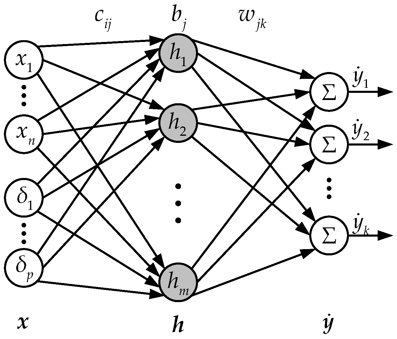
In this work, the nonlinear mapping to be approximated by the network is the mapping from the state and control vector pair to the state time derivatives, i.e., the mapping F of Equation (14). A radial basis function neural network (RBFNN) is adopted to accomplish the work in this paper. The network structure is shown in Figure 1.
The network can be represented as
y ˙ = f s N N x , u = W s N N T h x , u
h j x , u = exp [ x , u ] c : , j 2 2 b j ,           j = 1 , 2 , , m
in which the network input is the state-control vector pair [ x , u ] = [ p , , φ , , u , , δ c o l , , δ a i l , , δ I S ] T 18 , and the network output is the selected state variables of particular interest, which in the application of inner-loop RCAH controller design is the angular rate derivatives y ˙ = [ p ˙ , q ˙ , r ˙ ] T 3 . The hj is the output of the j’s Gaussian basis function, c : , j 17 × 1 and b j are the respective center coordinates and the width of the j’s basis function, and W s N N T 3 × m is the time-invariant network weight matrix. The network should be trained offline by the data covering the desired flight envelope derived from the flight dynamics model of the tiltrotor aircraft obtained from previous sections. It is worth noting that the training data should cover all of the valid ranges of each control deflection.
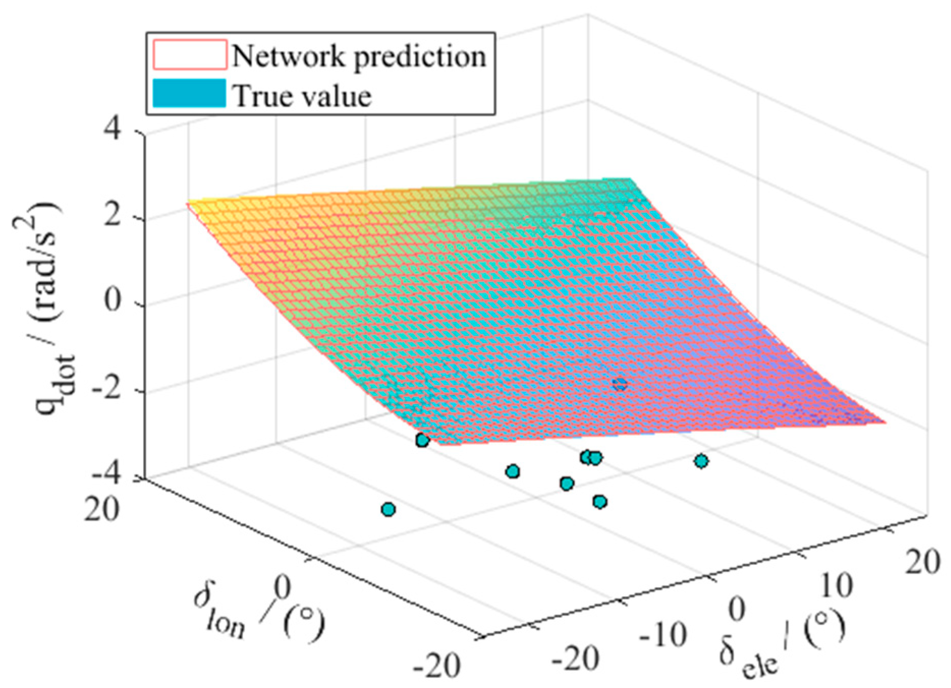
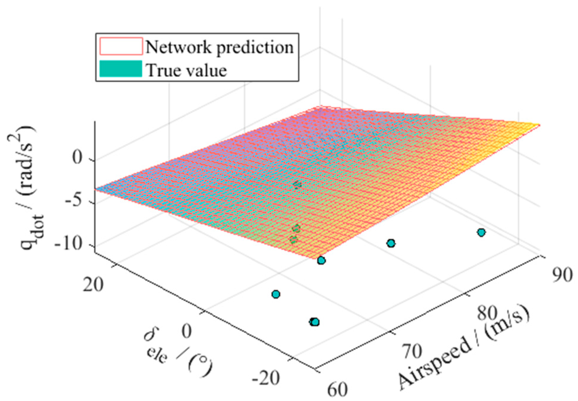
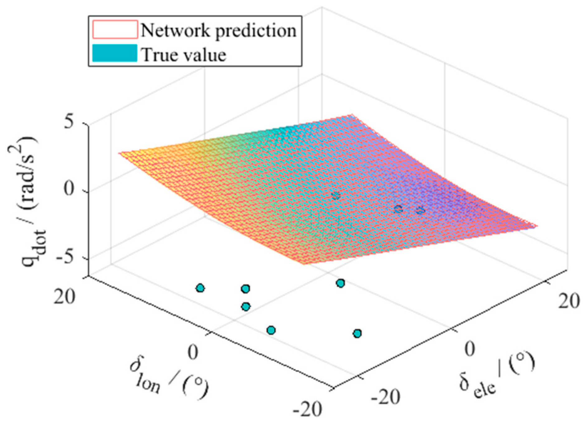
In this work, to study the model approximation of a tiltrotor aircraft during conversion mode, the dynamic tilting of the rotor nacelles is of great importance. In this case, two typical nacelle angles will be selected. Considering the dynamic tilting, although these two cases are fixed nacelle angles, the model to be approximated is by no means static. The training data of the network are obtained from the dynamics models rather than trimmed static models. This can be explained by the non-zero state derivatives, i.e., the output of the network contains all possible values of the pitching rate. In the meantime, under practical applications, the input of the actual network will not contain only discrete points of nacelle angles but rather a continuous range from 0 deg to 90 deg. The choice of these two angles is for the convenience of illustrating the basic idea of the article.

3. Optimization of the Neural Network Sample Distribution Pattern

With a uniformly distributed sample pattern, the total number of training set data points would be as many as 95 for each network output under the condition that only five points are selected for each flight state and control. This would be challenging for both the computer memory size and the total training time. As a result, in order to save computational resources and reduce the total CPU time, it is desirable to exploit the limited number of sample points.
On closer inspection of the resultant mapping of Section 2.2, one can find the characteristics of the ‘response surface’, which is the curvature of the surface that is often not identical throughout the domain. This resulted in the fact that each aerodynamic component of the aircraft is modelled with a different mathematical complexity. For example, helicopter rotor forces and moments intrinsically nonlinearly depend on its rotor controls, while forces and moments produced by the fixed-wing control deflections are linearly modelled by factors of control effectiveness. This, under a point of view of regarding the aircraft model as its state-derivative field (i.e., F ( x , u ) in Equation (14)) in a vector space of its state-control pair, will lead to the fact that the gradient field of F is non-uniform. Under this circumstance, in order to obtain an optimum result of network training, sample points should be distributed densely in the region where F ( x , u ) varies drastically. In the region where the gradient is nearly uniform, fewer sample points should be adequate to obtain a desirable network Mean Square Error (MSE).

3.1. Problem Formularization and Methodology

Through the above statement, the subject can be considered to find the optimum distribution pattern of the sample points, that is to say, the best combination of network input variables through which one can obtain a trained network with a minimized MSE, and this can be formulated by a non-convection optimization problem as follows:
minimize f M S E A s N N D D = x ( n ) , u ( n ) T , y ˙ ( n ) n = 1 N x ( n ) = [ x 1 ( n ) , , x 9 ( n ) ] T u ( n ) = [ δ 1 ( n ) , , δ 9 ( n ) ] T y ˙ ( n ) = F x ( n ) , u ( n ) subject   to x i min x i ( n ) x i max ,   i = 1 , , 9 δ j min δ j ( n ) δ j max ,   j = 1 , , 9
in which the optimization objective is the MSE of the trained network provided by the training algorithm A s N N ( ) , D is the set of training samples of size N, x(n) and u(n) are the sampled network inputs, and y ˙ ( n ) is the corresponding output.
The particle swarm optimization (PSO) algorithm proposed by Eberhart and Kennedy [24], as one of the most well-regarded swarm intelligence algorithms, was inspired by the foraging of bird flocks. With the following rules, i.e., (1) each bird flies toward the individual closest to itself and avoids collision; (2) the flock flies toward a food source; and (3) every bird tends to the center of the flock, the PSO algorithm searches the global optimum of every iteration. Like other metaheuristic algorithms, this scheme avoids being trapped by the local optima through a stochastic operator on each individual’s velocity vector, specifically by randomly altering the ratio of its social learning and self-recognition factors (CSR and CSL, respectively):
v i N + 1 = C I W v i N + C S R r a n d S R P i b e s t N P i N + C S L r a n d S L P g b e s t N P i N
In this work, instead of the standard PSO algorithm, an improved differential evolutionary particle swarm optimizer based on the fourth-order Runge–Kutta algorithm (DPSORK) is adopted to accomplish the above sample pattern optimization task. The scheme is derived from the general differential PSO model:
v ˙ i = C I W 1 v i Φ P i + Φ S R P i b + Φ S L P g b P ˙ i = C I W v i Φ P i + Φ S R P i b + Φ S L P g b Φ S R = C S R r a n d S R Φ S L = C S L r a n d S L Φ = Φ S R + Φ S L
In the above model, v ˙ i and P ˙ i are the velocity and position of the ith individual at the current time (iteration), CIW, CSR, and CSL are the respective inertia weight, self-recognition, and social learning factors, rand is the uniformly distributed random number between [0,1], and Pib and Pgb are the optima encountered by the individual itself and by the flock in history (global optimum). Viewed as ordinary differential equations, the above model can be solved by several different numerical methods, which results in variants of schemes. A fourth-order Runge–Kutta method is adopted for its relatively high order of truncation error. Thus, the scheme with a step size of h can be represented as
v i N + 1 = v i N + h 6 K 1 + 2 K 2 + 2 K 3 + K 4 P i N + 1 = P i N + h 6 L 1 + 2 L 2 + 2 L 3 + L 4 K 1 = C I W 1 v i N Φ P i N + Φ S R P i b + Φ S L P g b L 1 = C I W v i N Φ P i N + Φ S R P i b + Φ S L P g b K 2 = C I W 1 v i N + h 2 K 1 Φ P i N + h 2 L 1 + Φ S R P i b + Φ S L P g b L 2 = C I W v i N + h 2 K 1 Φ P i N + h 2 L 1 + Φ S R P i b + Φ S L P g b K 3 = C I W 1 v i N + h 2 K 2 Φ P i N + h 2 L 2 + Φ S R P i b + Φ S L P g b L 3 = C I W v i N + h 2 K 2 Φ P i N + h 2 L 2 + Φ S R P i b + Φ S L P g b K 4 = C I W 1 v i N + h K 3 Φ P i N + h L 3 + Φ S R P i b + Φ S L P g b L 4 = C I W v i N + h K 3 Φ P i N + h L 3 + Φ S R P i b + Φ S L P g b
In the above scheme, for a better and rapid convergence, parameters CIW, CSR, and CSL of the optimizer are incorporated with the following time-varying form:
C j = C j , i C j , f N max N N max + C j , f ,   j = I W , S R , S L
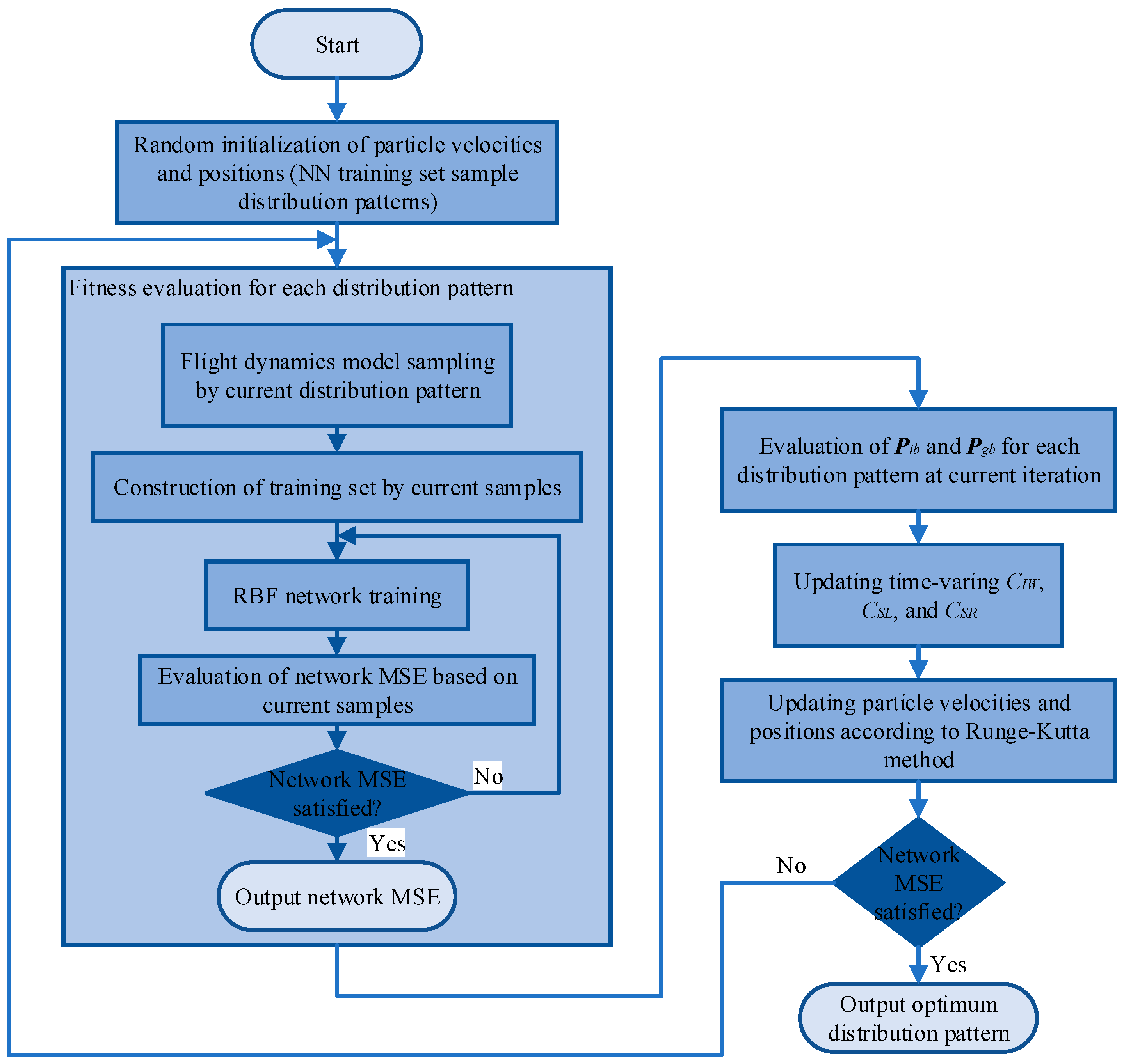
The procedure of optimization of the network training set sample distribution pattern is shown as Figure 2.

3.2. Case Studies

3.2.1. Approximation of a Nonlinear Function

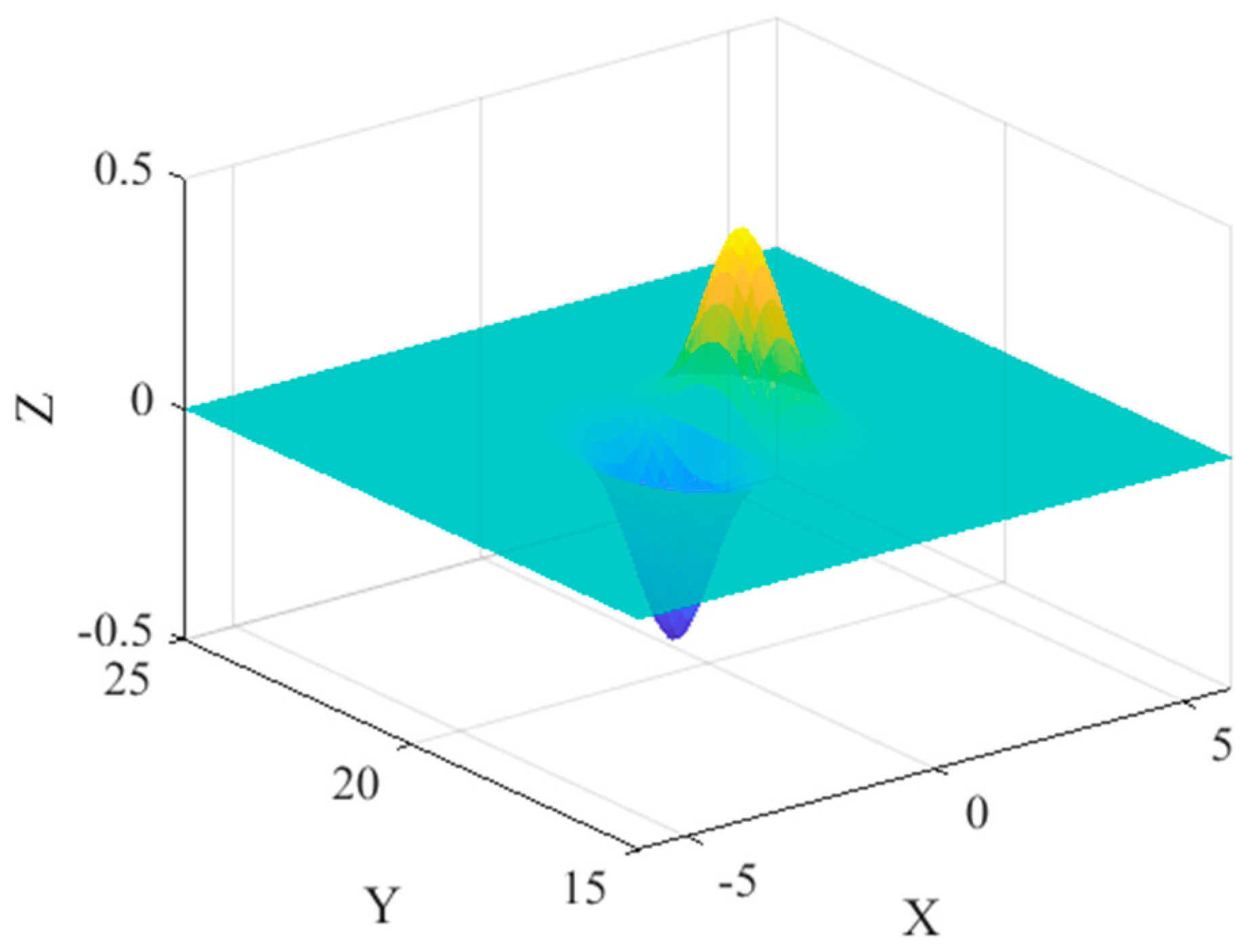
To further explain the principle of the methodology presented in the previous section, an example case is discussed by the approximation of the objective function:
z = x exp x 2 y 20 2
The function plot is shown in Figure 3. The neighborhoods of its two maxima (the two ‘spikes’ on the function plot) are the primary concern indicating the optimization results where the distribution pattern should condense its samples. A total sample number is confined to 40 points in this task. The parameters of the optimizer are summarized in Table 1.
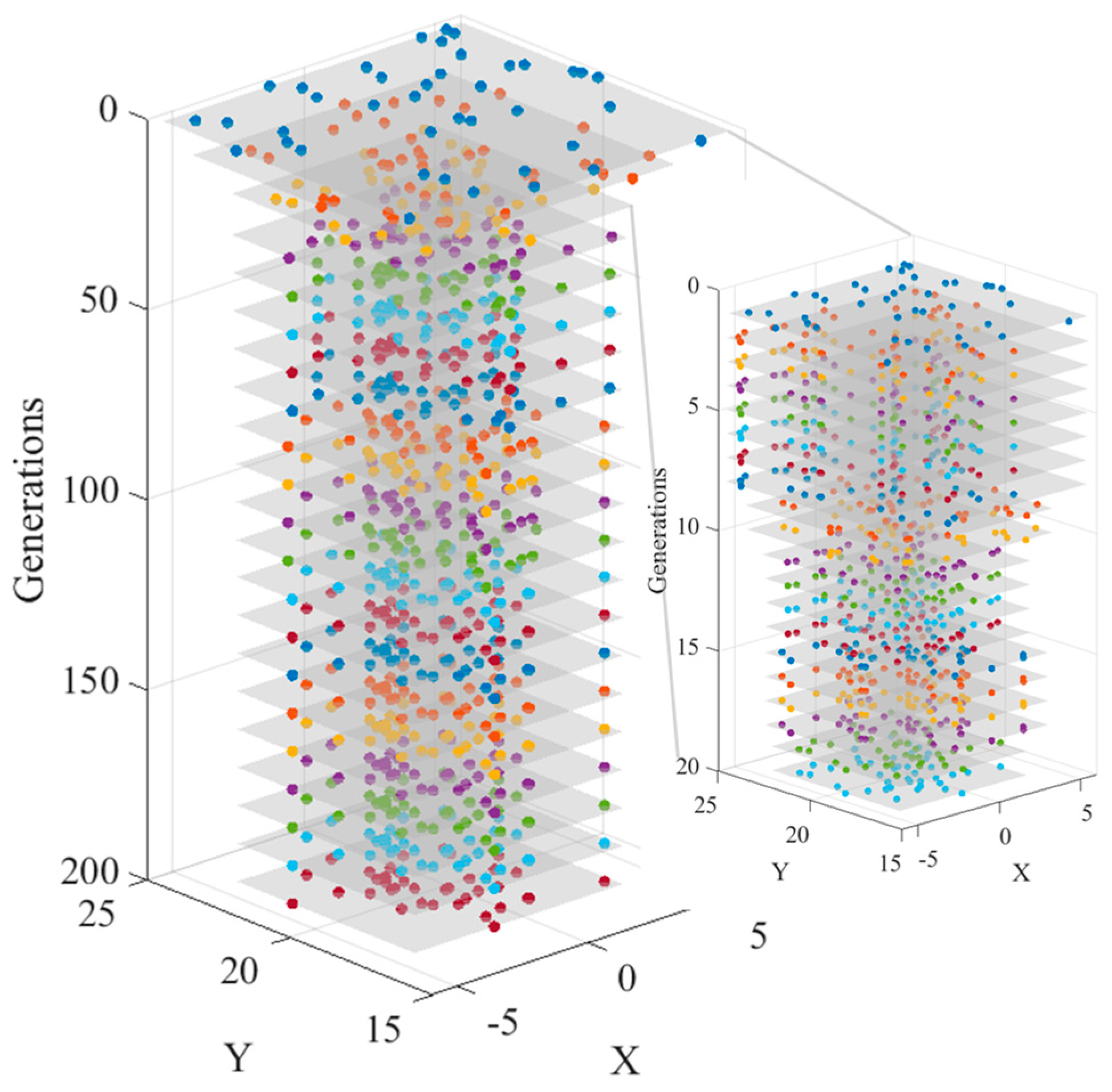
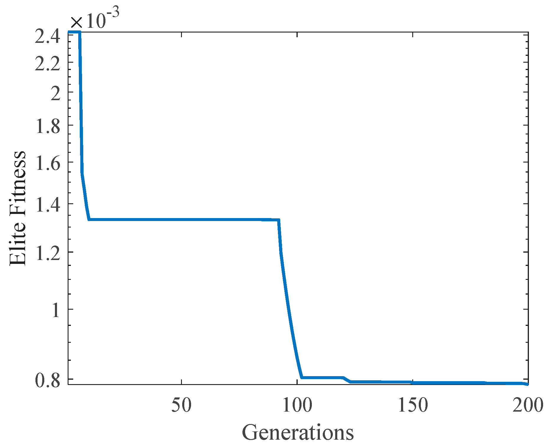
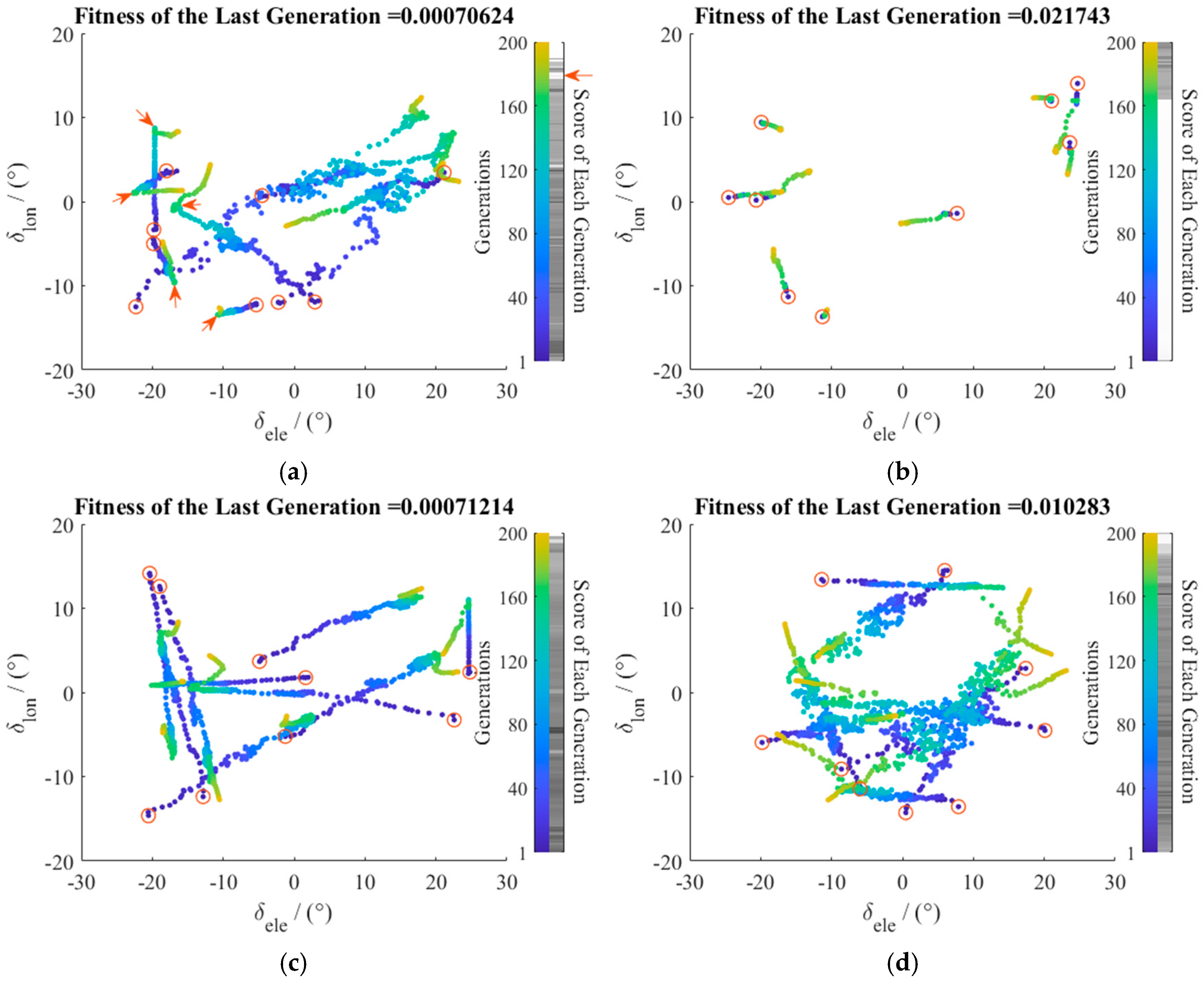
The convergence history of the elite from each generation is presented in Figure 4. Colored dots on the shaded plane denote the best sample points of each generation. From the right-sided details of the first twenty generations, one can find from the evolution process that the distribution pattern indicates an obvious tendency of the concentration of sample points from a uniformly random distribution on the XY plane to the two ‘spikes’ of the objective function. These ‘spikes’ are exactly where the gradient varies drastically. On the contrary, from the region where the surface is relatively ‘flat’, fewer sample points are selected.
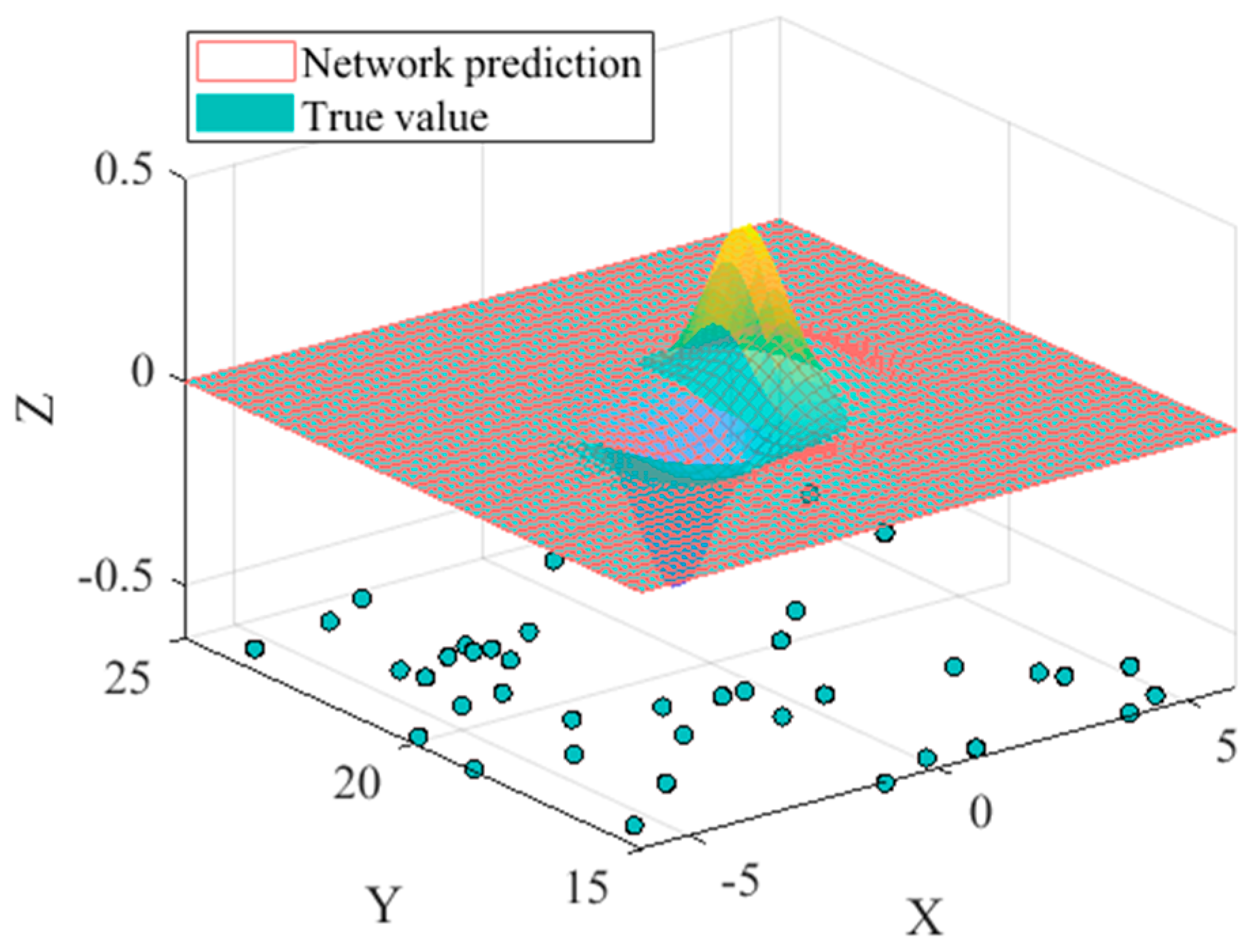
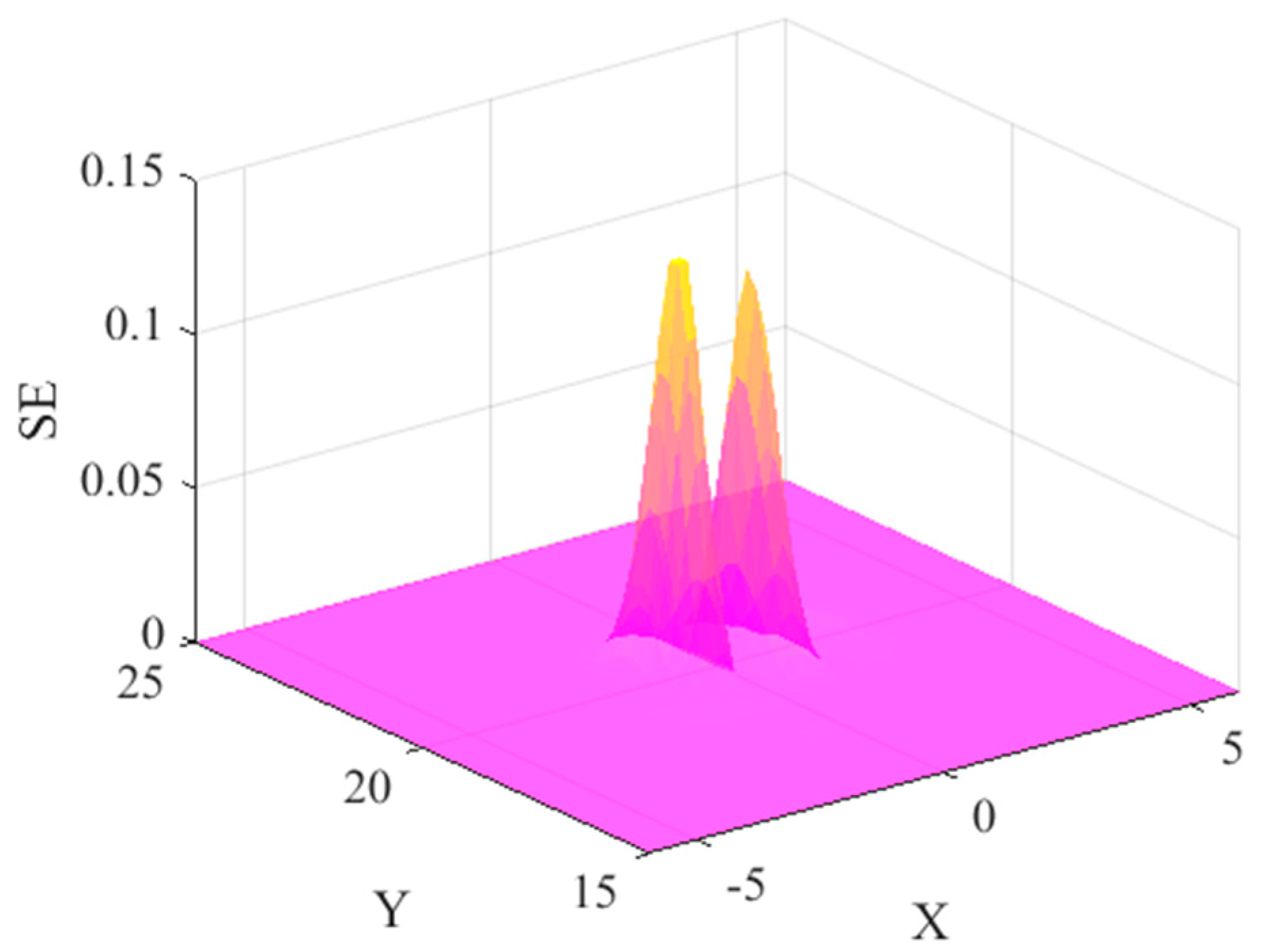
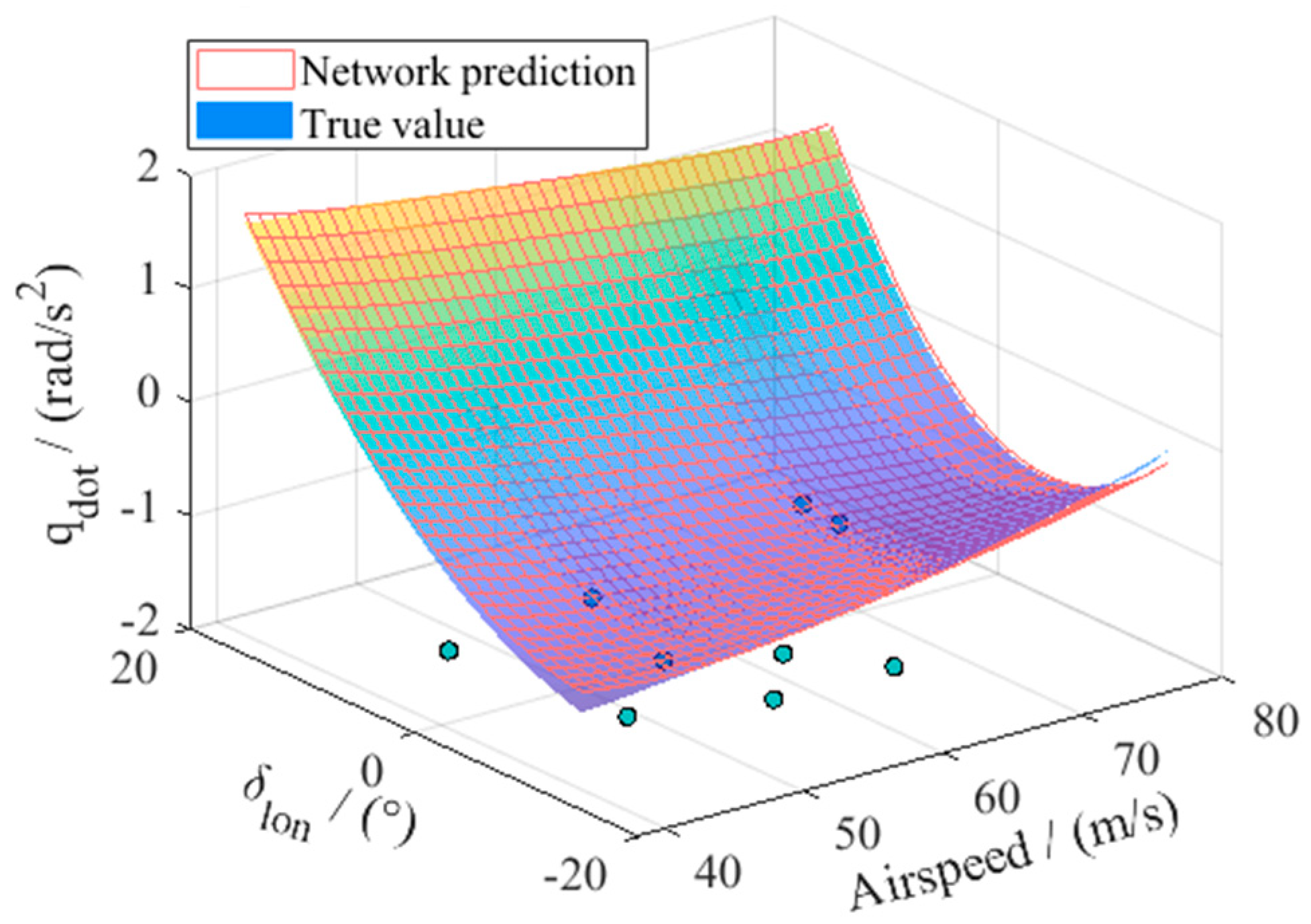
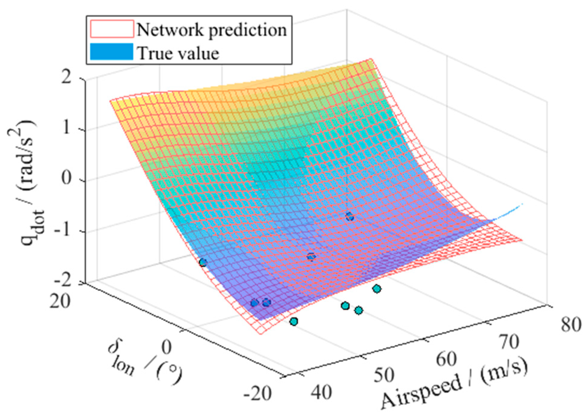
The network trained from the optimum sample pattern was simulated, and the result is shown by Figure 5. The true values obtained by sampling the objective function are shown by the colored surface, while the network prediction at the same sample points is shown by the mesh grid. As a result, the pattern optimized by DPSORK can be used to obtain an RBF network approximating the example function with relatively high accuracy. The global network square error (SE) distribution is shown in
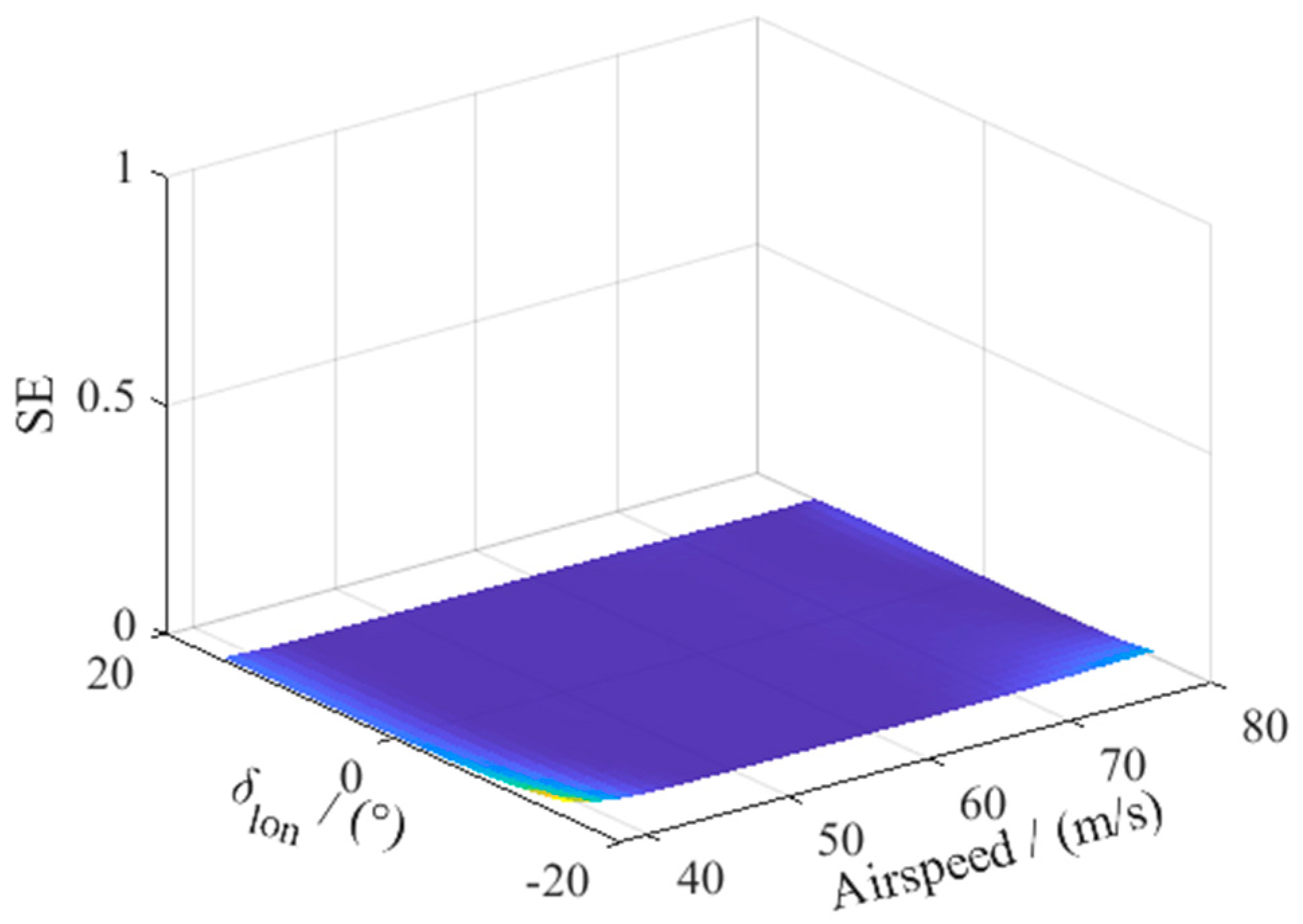
 Figure 6.
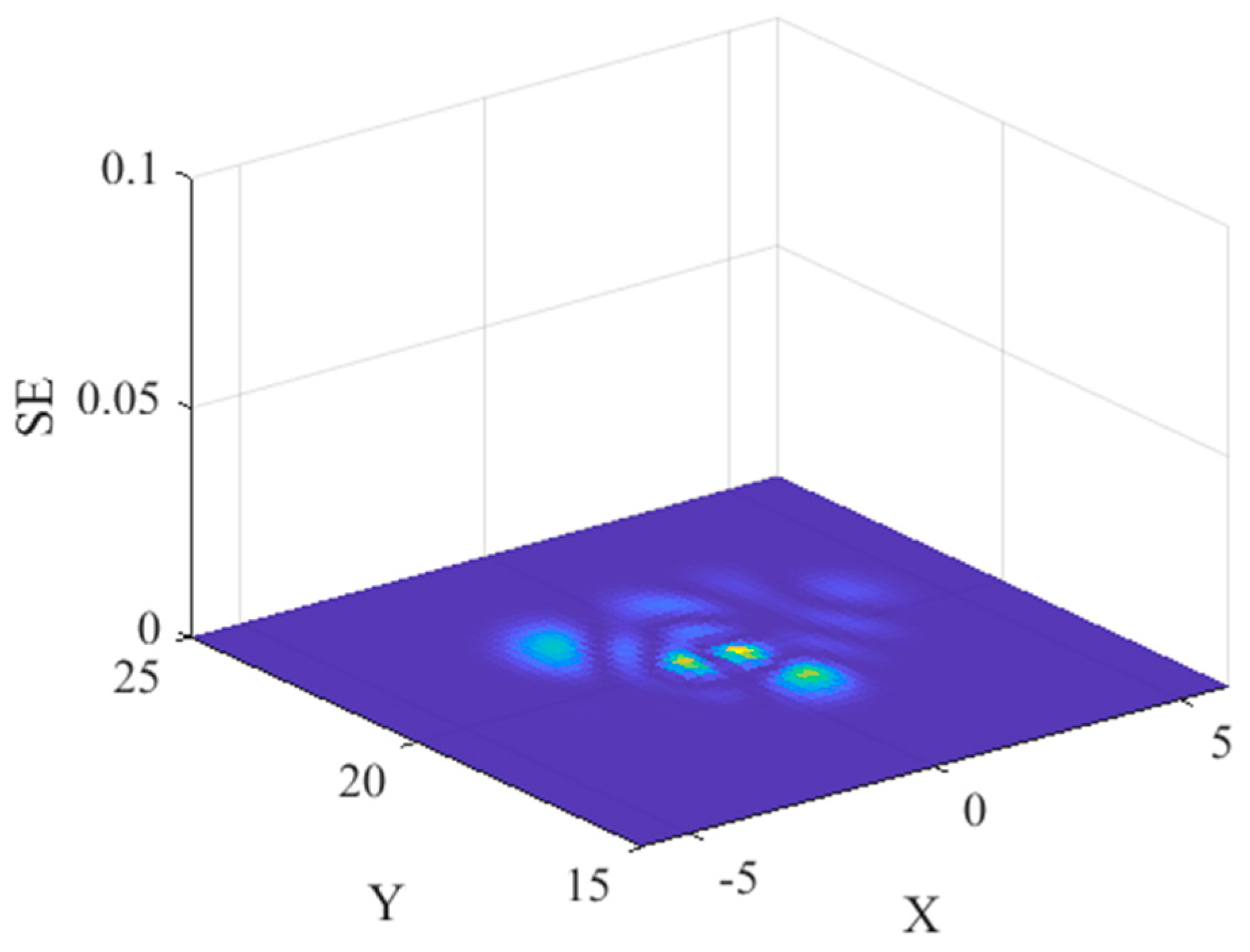
In the meantime, a comparative network trained by randomly selected samples uniformly distributed on the problem domain is simulated in 
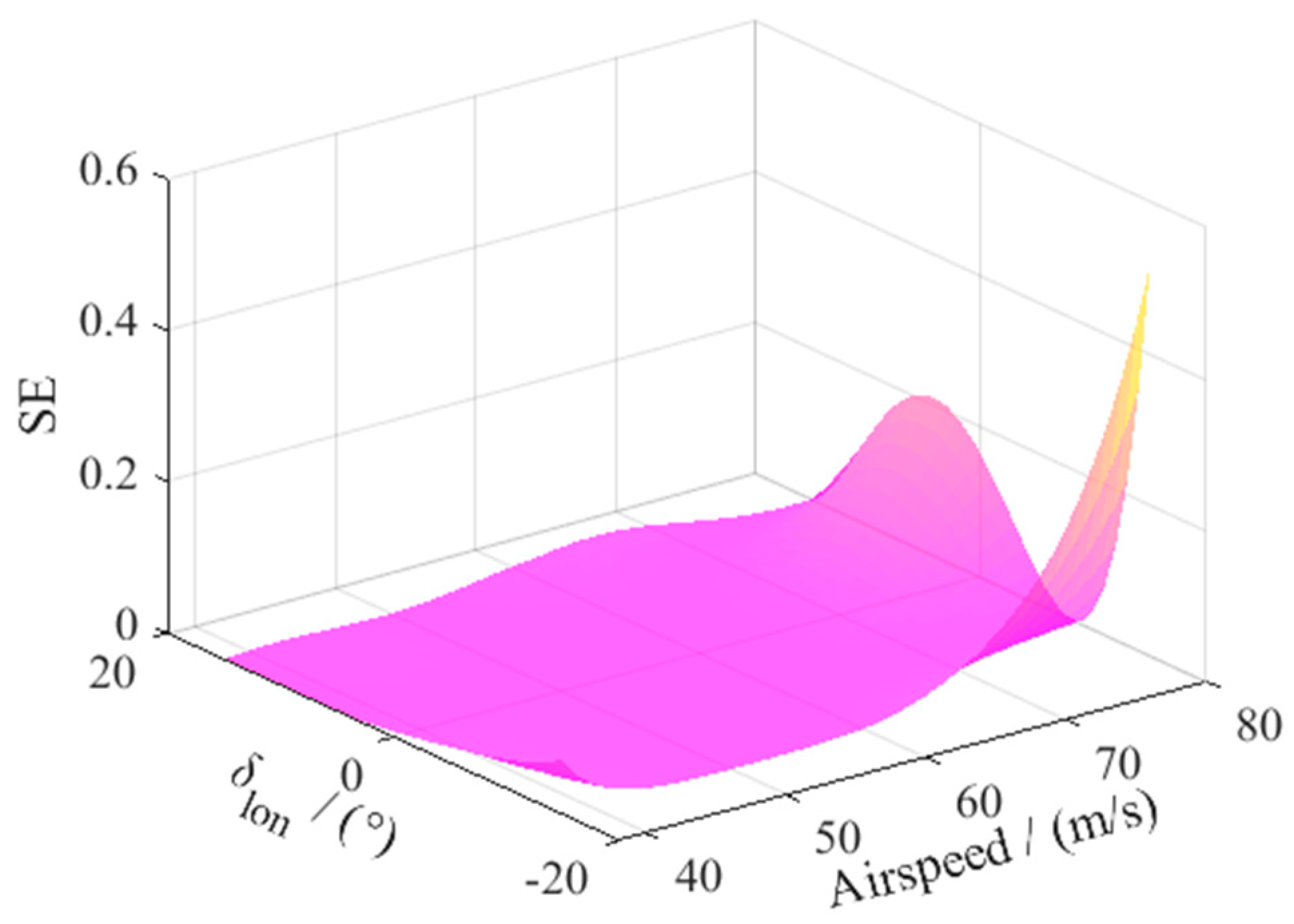
Figure 7. Obvious error can be seen between the predicted value and true value. From the global SE distribution shown in Figure 8, one can find that the large values of SE are primarily around the two ‘spike’ regions of the objective function domain because of a lack of adequate amount of sample points allocated to these regions.

3.2.2. Parameter Analysis for Searching the Particle Number and Sample Number

To reveal the impact of algorithm parameters including searching the particle number and sample number, repeated averaging simulations were performed. First, the particle number was fixed at 20, and the sample points increased from 10 samples to 140 samples. Every case was repeated 30 times to exclude the randomness of performance. The results are shown in Figure 9. The left part indicates the convergence history of the elite population of each generation. Different colors indicate result from different sample point numbers on the graph. The right part of the figure is the average and dispersion of the elite fitness of the last generation, and the averages are indicated by the diamond marker while the error bars showed the maximum and minimum values of the 30-repeated simulations. As a result, under the same amount of searching particles, the sample point number has a major impact on the convergence performance, and after 40 samples, the influence of the sample point number can be regarded as negligible.
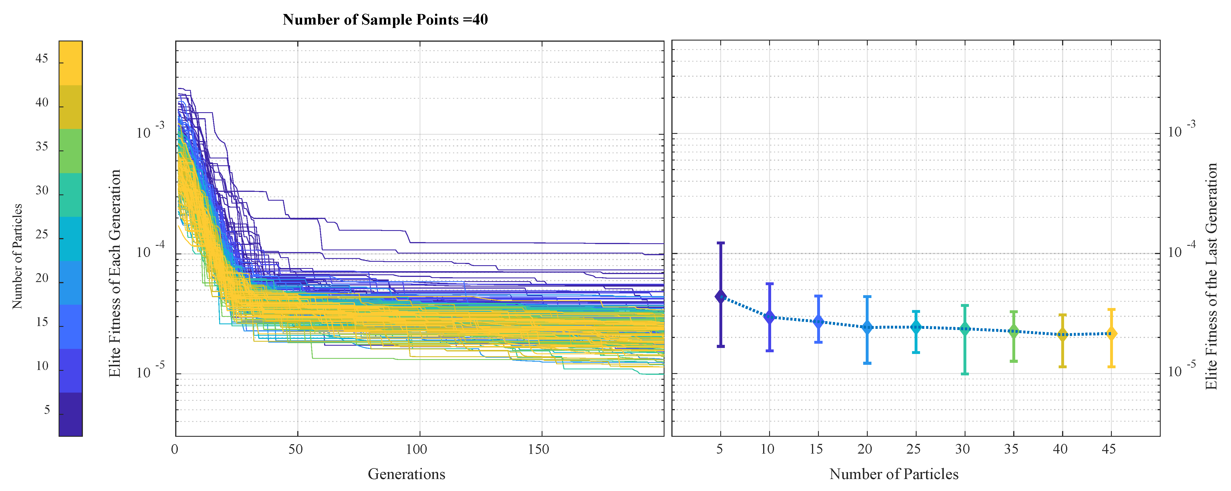
Secondly, the sample point number was fixed at 40 to study the impact of searching particle numbers. With the same procedure, the searching particle number increased from 5 to 45, and each case (the same number of particles) was repeated 30 times. The results are shown in Figure 10. From the convergence history below, one can find that the searching particle number has a minor influence on the overall precision after convergence. Both average fitness and dispersion are affected weakly by the particle number, especially for those cases with a particle number greater than 10. As a result, a combination of 40 sample points with 20 searching particles was selected in this work.

3.2.3. Time Domain Response Performance

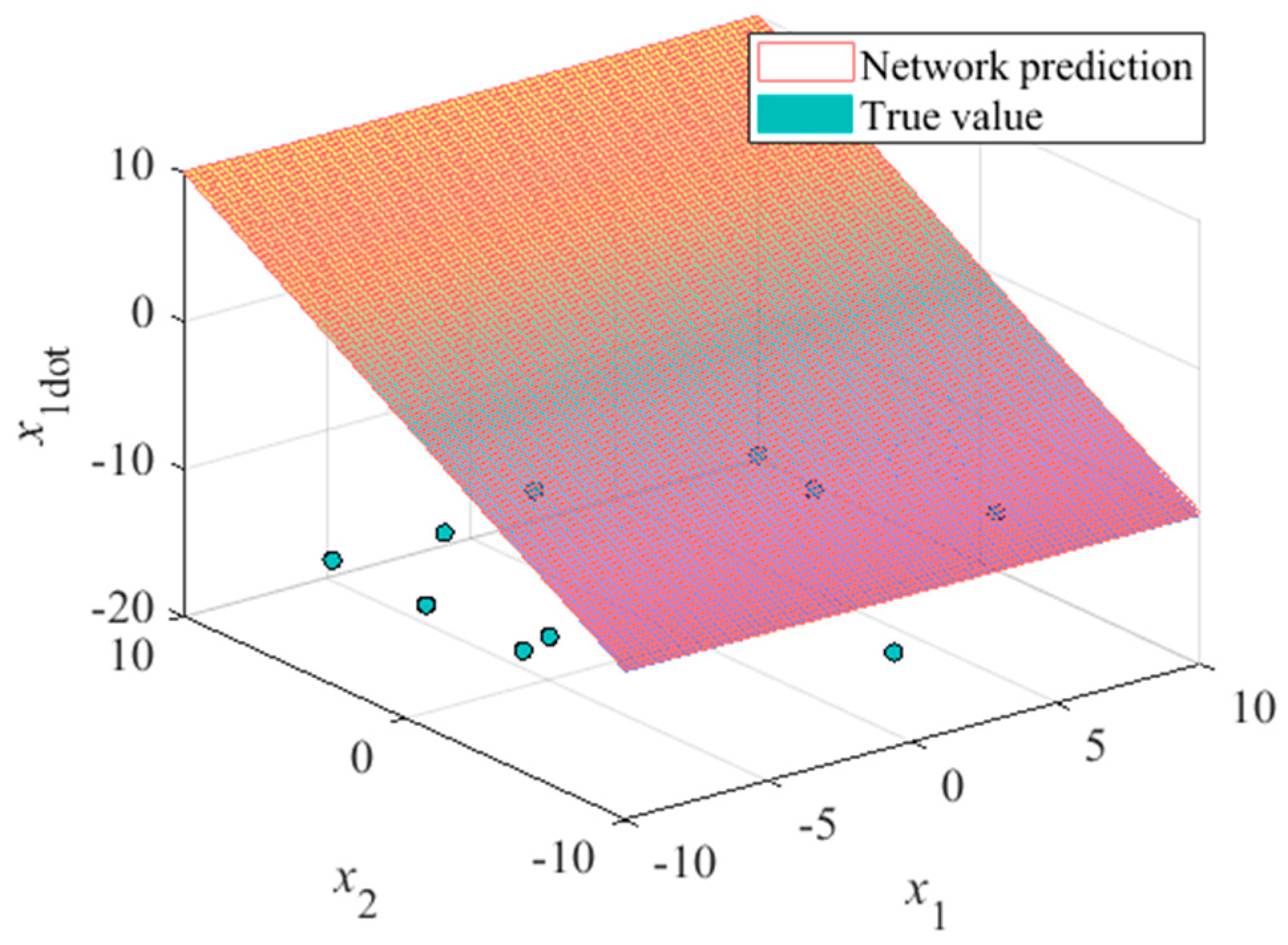
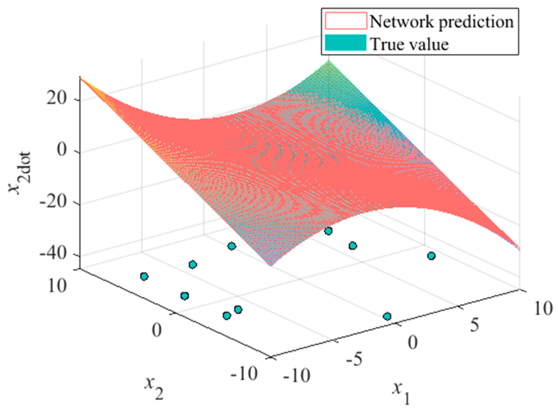
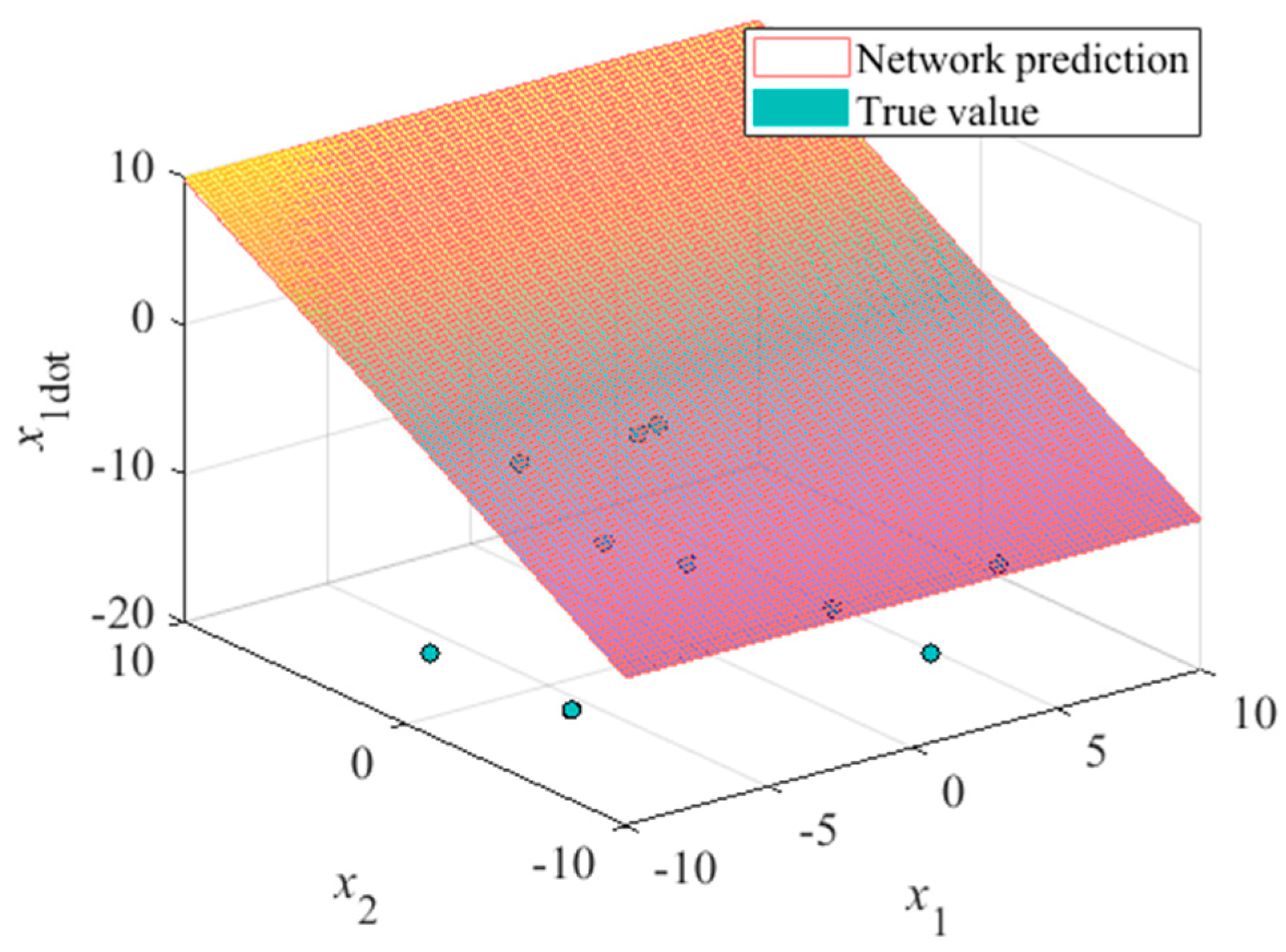
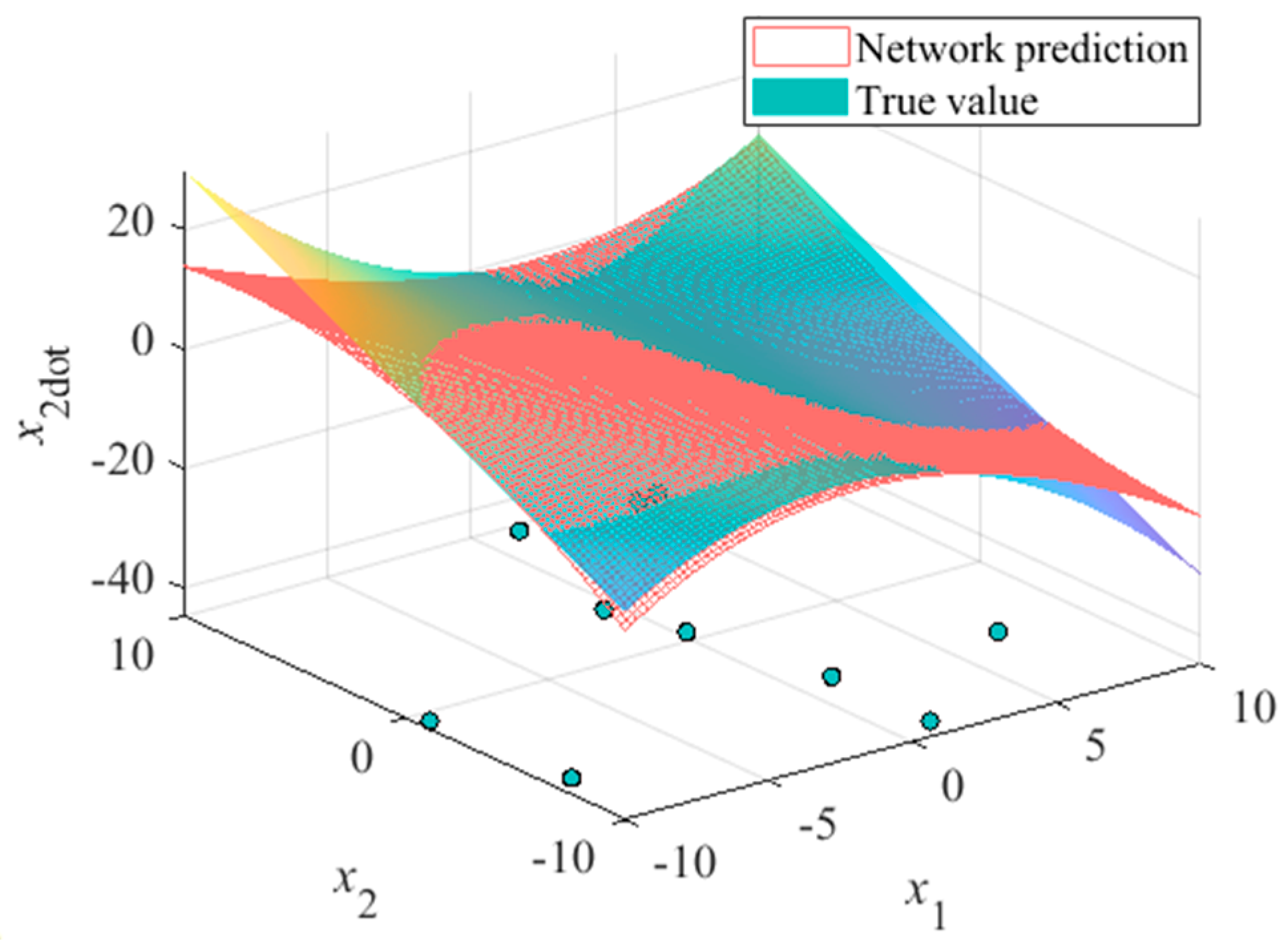
To illustrate the approximation performance of the presented optimization algorithm for an unstable nonlinear multi-variable dynamic system, this subsection selects a Van der Pol oscillator as the example, and the time-response of the system is shown. The Van der Pol oscillator is a representative nonlinear autonomous dynamic system with two states. The system equations can be written as
x ˙ 1 = x 2 ; x ˙ 2 = x 1 0.02 1 x 1 2 x 2
A total number of 10 sample points on the state space was restricted to this task. The comparative results of the network-approximated Van der Pol system derivatives are shown in Figure 11, Figure 12, Figure 13 and Figure 14. The global MSE of these networks with multiple outputs is the sum of all outputs, i.e., state derivatives. The x ˙ 1 field of the Van der Pol oscillator is a flat surface with respect to its two states, which can be seen from the system equation, so the approximation precision can be relatively high even under the random sample case (seen in Figure 13). The approximation of the x ˙ 2 field, however, shows a low performance if the training set has not been optimized (see Figure 12 and Figure 14).
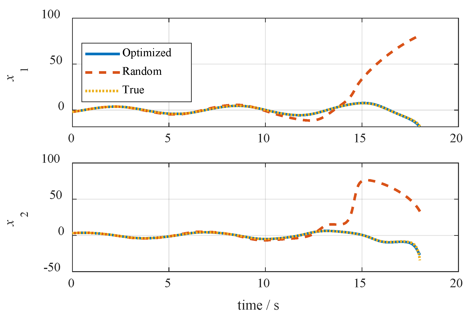
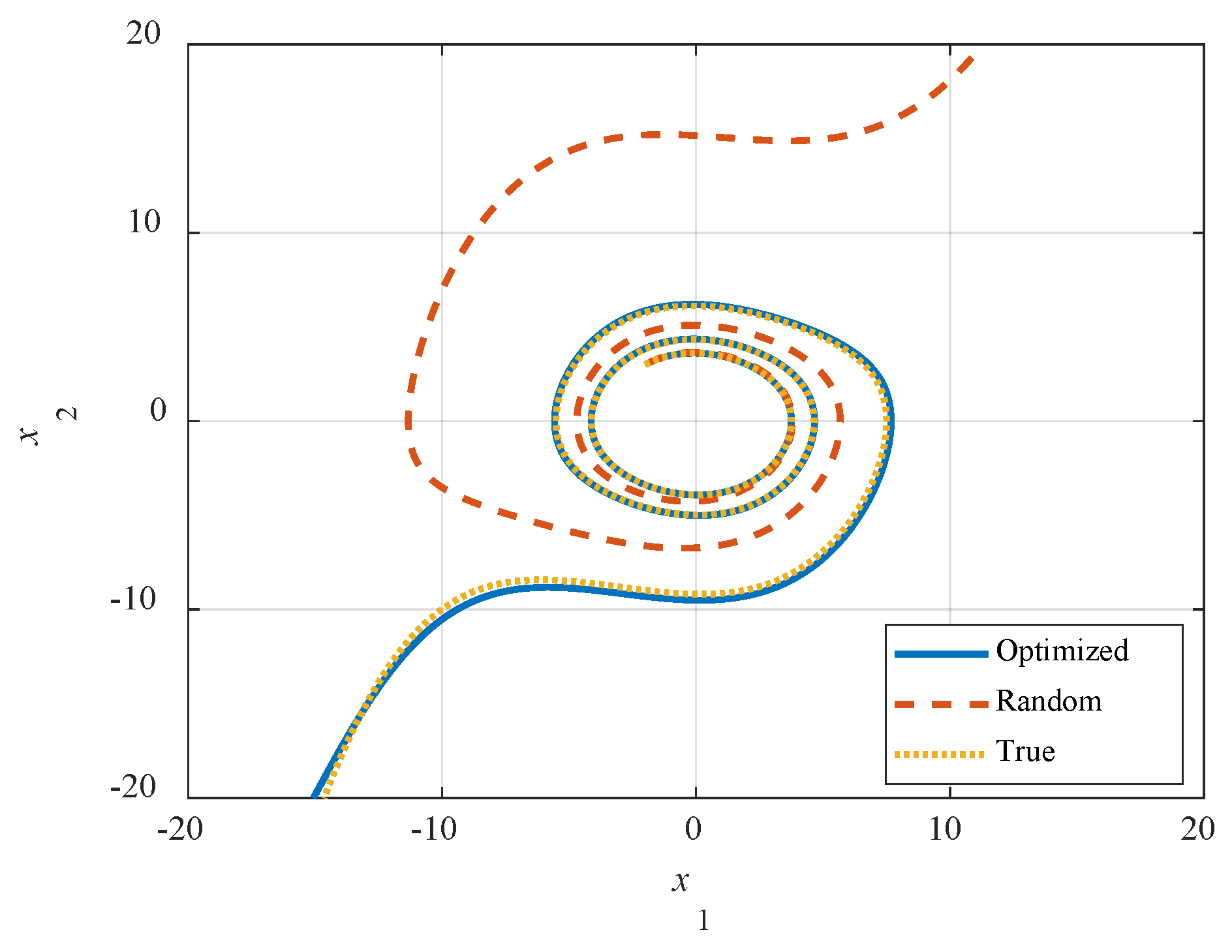
Simulation was performed on the optimum network obtained by the presented algorithm, the random set-trained network, and the true system, and a fixed-step Runge–Kutta solver with a 0.01 s time step was adopted. Results are shown in Figure 15 and Figure 16; Figure 15 depicts the time response of the two state variables, and the system phase portraits are shown in Figure 16. From these results, the optimized approximation system coincided with the actual system, and the nonlinearity and unstableness were reconstructed well by the optimized neural network.

4. Sample Distribution Pattern Optimization for the Flight Dynamics Model of a Tiltrotor Aircraft

4.1. Results of the Early-Stage Conversion Mode

The research aircraft of this work is the Bell XV-15 tiltrotor aircraft. Three views are shown in Figure 17 below. The parameters of the vehicle are summarized in Table 2.
The early stage of the tiltrotor conversion mode, represented by a 30 deg nacelle tilting angle, is considered. Since the primary control of the longitudinal channel in this stage is the helicopter rotor longitudinal cyclic pitch, the first model to be approximated by the neural network is the dependence of the longitudinal body axis pitching acceleration, q ˙ , on the longitudinal control and airspeed. An available rotor cyclic pitch range of −15 deg to 15 deg and an airspeed range of 37.9 m/s to 79.6 m/s (within the conversion corridor) are selected for simulation. The conversion corridor is obtained by the lower and upper boundaries of the trimmed airspeed-tilting angle scheme, in which the lower boundary represents the fixed-wing stall. An upper engine power boundary is obtained by manually selecting a maximum airspeed since the engine is not modeled in this work, which is not of great importance in clarifying the approach of this work.
The following Figure 18 depicts the q ˙ -field with respect to the above stated variables. The true values directly sampled from the flight dynamics by a data set of an interval of 1 deg longitudinal and that of 1 m/s are depicted by the colored surface. The network is trained by an optimum sample pattern obtained by 200-generations DPSORK searching (shown by the green dots on the q ˙ = 4       rad / s 2 plane) in which a total number of nine sample points is confined and is then sampled by a set with the same interval as above, shown by the red mesh grid. From the simulated network, the MSE is as low as 9.9 × 10⁻⁴. The global SE distribution of the optimum network is shown in Figure 19. The elite fitness values from 200 generations are shown in Figure 20, from which one can find rapid convergence within the first 10 generations.
As a comparison, a network trained by nine randomly selected sample points uniformly distributed on the problem domain is also simulated, with results shown in Figure 21 and Figure 22. A relatively low performance is revealed by the random sample network, as the global MSE is 0.018. From the result of the random sample network, one can find that large deviation occurs in the region where the gradient varies drastically (i.e., high airspeed with a negative longitudinal cyclic pitch), and the sample points are relatively sparse.
In the meantime, the elevator, as a redundant control, is considered with the longitudinal cyclic in the early conversion stage. The elevator control deflection is restricted to −25 deg to 25 deg in this task. The simulation results of the trained network are shown in Figure 23. From the network predictions, one can find that the nonlinearity of q ˙ with respect to the controls on the longitudinal control axis mainly depends on the helicopter controls.

4.2. Results of the Late-Stage Conversion Mode

The training sets of the late stage of the tiltrotor are sampled under a condition of a 70 deg nacelle tilting angle. In the late stage of the conversion mode, the aircraft exhibits characteristics closer to those of the fixed-wing airplane. The same longitudinal q ˙ -field is considered. The primary control in the longitudinal channel is the fixed-wing elevator deflection, whereas the rotor longitudinal cyclic control is the redundant control. For the dependence of q ˙ on the airspeed, the airspeed range is chosen from 64 m/s to 90 m/s, within the conversion corridor.
The simulation results of the optimum network-approximated q ˙ -field with respect to airspeed and elevator deflection are shown in Figure 24. The q ˙ -field dependency on the elevator deflection and longitudinal cyclic pitch is depicted in Figure 25. Relatively good results are obtained by the optimum sample network.
The searching loci of the last task are shown in Figure 26, from which the two important stages of metaheuristic algorithms can be seen: the exploration phase and the exploitation phase. Four typical particles are chosen, including the one that has reached the optimum location (see Figure 26c, global best location at its 199th generation). Colored scatter points on the plot denote the particle position for each generation (searching loci), with the generation number depicted by color. Points marked by red circles denote the locations of the initial searching points of each particle. The grey-scale color bar shows the score of each generation of particle corresponding to the generation bar on its left. The particle score is calculated by its fitness value normalized by the global best and worst values and then scaled by the common logarithm; black denotes the worst fitness, and white denotes the best fitness. The advantage of not being trapped in local minima can be seen in Figure 26a, in which a local minimum is marked by the arrow beside the grey score bar. The algorithm is able to jump out of the local minimum stochastically, which is shown by some sharp turns on the searching loci (marked by the arrows). The final convergence of the searching process, however, cannot be guaranteed by the initial closeness to the global optimum locus of a single particle. As shown in Figure 26b, the particle is relatively close to the optimum in the first generation, but it deviates from the best location after the 160th generation. This is also attributed to the stochastic nature of the DPSORK. In general, the overall searching process shows different searching patterns, as can be seen in Figure 26c,d, in which particle No. 4 shows a predominant effect of inertia by its relatively ‘straight’ locus whereas particle No. 20 exhibits more stochastic behavior by its scattered distribution of search points in a relatively large search area. This behavior can be found in both cases of different particles and within one single particle, see Figure 26a.

4.3. Time-Domain Response Simulation

To illustrate the time response performance of the approximated model, this subsection takes a longitudinal short-period approximation of the tiltrotor as an example. The flight state variables considered are the body axis velocity w and angular rate q, with the control variable longitudinal cyclic pitch δ l o n . The truncated longitudinal short-period nonlinear model can be represented as
w ˙ = f w w , q + g w δ l o n q ˙ = f q w , q + g q δ l o n
The training data of the nonlinear state functions fw, fq, and control functions gw, gq are sampled from the full-state nonlinear tiltrotor model under its conversion mode of a 30 deg nacelle tilting angle. The forward velocity u = 59 m/s, which is considered to remain nearly constant during short-period oscillation. All of the lateral state and control variables are fixed at zero, as well as the redundant controls in the longitudinal channel. The simulation is started under a non-equilibrium flight condition. The control signal of a bipolar square wave of longitudinal cyclic control is imposed at simulation time t = 2 s, see Figure 27.
Figure 28 shows the longitudinal truncated short-period mode time response under the above command. Optimized and random networks are both trained by a set of 17 sample points, in the state-control space of 10       m / s w 17       m / s , 3       rad / s q 3       rad / s , and 15       deg δ l o n 15       deg , with derived networks with 16 neurons in the radial basis layer. From the simulation results below, the optimum trained network coincides better with the actual tiltrotor model, which shows a much better time response performance than the random sample network. This verifies the availability and effectiveness of the presented method applied to the approximation of a nonlinear rotorcraft flight dynamics model.

5. Discussion and Conclusions

Against the background of the extensive use of neural networks to approximate a flight dynamics model in the design process of tiltrotor aircraft, this paper presented, with the aid of a swarm intelligence algorithm, the methodology to solve the practical problem faced by network training, that is, the requirement of a tremendous amount of training set data points in order to obtain a satisfactory training result. Constrained by the hardware computing power at hand, the total number of training set data points is limited to some extent. In this case, the major problem solved by this article is addressed by how to exploit the limited number of training data points. The results of this work can be summarized as follows:
(1)
For the function approximation problem, this work presented a novel methodology, that is, to use the metaheuristic optimization algorithm to search the optimum sample pattern of the training set, revealing its effectiveness and benefits. In the example case of approximating a highly-nonlinear function with two inputs, the RBF neural network trained by the optimum data set obtained by the DPSORK algorithm showed a significantly improved performance, with a network MSE decrease from 2 × 10⁻³ to 3 × 10⁻⁵ (65 times lower) compared to the results of the random sample network.
(2)
The DPSORK-optimized RBF neural network was applied to the flight dynamics model approximation of the pitching angular acceleration field of the tiltrotor aircraft. Examples of the early (30 deg nacelle tilting angle) and late stage (70 deg nacelle tilting angle) of its conversion mode were studied. The methodology presented in this work showed its generality and readiness of solving practical problems.
(3)
Although the overall error of the approximated network has been reduced by the presented algorithm, there are still certain deviations in each case (for example, the MSE of 8.7 × 10⁻⁴ for control response at the late tilting stage). Since an RBF network is able to converge on a result with an arbitrarily small deviation with adequate neurons, the remaining problem would be to decrease the deviation under a neuron number as low as possible. Future work should study all of the parameters (including that of self-recognition and social learning factors) analytically and formulate the optimum of these parameters with respect to the studied cases.

Author Contributions

Conceptualization, J.W. and Y.S.; methodology, J.W.; software, J.W.; validation, J.W.; formal analysis, J.W.; investigation, J.W. and D.H.; resources, J.W. and C.Y.; data curation, J.W. and H.W.; writing—original draft preparation, J.W.; writing—review and editing, J.W., Y.S., H.W., D.H. and C.Y.; visualization, J.W.; supervision, Y.S., H.W. and D.H.; project administration, Y.S.; funding acquisition, Y.S. and C.Y. All authors have read and agreed to the published version of the manuscript.

Funding

This research was funded by the Jiangxi Province Key Research and Development Program: Research on Key Technologies of High-Speed VTOL Vehicles, grant number 20203ABC28W002.

Data Availability Statement

Data are contained within the article.

Conflicts of Interest

C.Y. is employed by the AVIC-Hongdu Ltd. The remaining authors declare that the research was conducted in the absence of any commercial or financial relationships that could be construed as a potential conflict of interest.

References

  1. Wang, Y.; Li, A.; Yang, S.; Li, Q.; Ma, Z. A neural network based MRAC scheme with application to an autonomous nonlinear rotorcraft in the presence of input saturation. ISA Trans. 2021, 115, 1. [Google Scholar] [CrossRef] [PubMed]
  2. Tang, D.; Tang, B.; Shen, W.; Zhu, K.; Quan, Q.; Deng, Z. On genetic algorithm and artificial neural network combined optimization for a Mars rotorcraft blade. Acta Astronaut. 2023, 203, 78–87. [Google Scholar] [CrossRef]
  3. Tee, K.P.; Ge, S.S.; Tay, F.E.H. Adaptive Neural Network Control for Helicopters in Vertical Flight. IEEE Trans. Control Syst. Technol. 2008, 16, 753–762. [Google Scholar]
  4. Razmi, H.; Afshinfar, S. Neural Network-Based Adaptive Sliding Mode Control Design for Position and Attitude Control of a Quadrotor UAV. Aerosp. Sci. Technol. 2019, 91, 12–27. [Google Scholar] [CrossRef]
  5. Tavoosi, J. Hybrid Intelligent Adaptive Controller for Tiltrotor UAV. Int. J. Intell. Unmanned Syst. 2021, 9, 256–273. [Google Scholar] [CrossRef]
  6. Yu, J.; Hesthaven, J.S. Flowfield Reconstruction Method Using Artificial Neural Network. AIAA J. 2019, 57, 482–498. [Google Scholar] [CrossRef]
  7. Alhazmi, N.; Ghazi, Y.; Aldosari, M.; Tezaur, R.; Farhat, C. Training a Neural-Network-Based Surrogate Model for Aerodynamic Optimization Using a Gaussian Process. In Proceedings of the AIAA SciTech 2021 Forum, Virtual Event, 26 August 2021. [Google Scholar]
  8. Seo, J.; Kapania, R.K. Development of Deep Convolutional Neural Network for Structural Topology Optimization. AIAA J. 2023, 61, 1366–1379. [Google Scholar] [CrossRef]
  9. Rostami, M.; Chung, J.; Park, H.U. Design optimization of multi-objective proportional–integral–derivative controllers for enhanced handling quality of a twin-engine, propeller-driven airplane. Adv. Mech. Eng. 2020, 12, 1687814020923178. [Google Scholar] [CrossRef]
  10. Wang, L.; Diskin, B.; Biedron, R.T.; Nielsen, E.J.; Bauchau, O.A. Evaluation of high-fidelity multidisciplinary sensitivity-analysis framework for multipoint rotorcraft optimization. J. Aircr. 2020, 57, 830–842. [Google Scholar] [CrossRef]
  11. An, J.Y.; Choi, Y.S.; Lee, I.R.; Lim, M.; Kim, C.J. Performance Analysis of a Conceptual Urban Air Mobility Configuration Using High-Fidelity Rotorcraft Flight Dynamic Model. Int. J. Aeronaut. Space Sci. 2023, 24, 1491–1508. [Google Scholar] [CrossRef]
  12. Chen, R.; Yuan, Y.; Thomson, D. A review of mathematical modelling techniques for advanced rotorcraft configurations. Prog. Aerosp. Sci. 2021, 120, 100681. [Google Scholar] [CrossRef]
  13. Rostami, M.; Bagherzadeh, S. Development and validation of an enhanced semi-empirical method for estimation of aerodynamic characteristics of light, propeller-driven airplanes. Proc. Inst. Mech. Eng. Part G J. Aerosp. Eng. 2018, 232, 638–648. [Google Scholar] [CrossRef]
  14. Xue, J.; Shen, B. A Novel Swarm Intelligence Optimization Approach: Sparrow Search Algorithm. Syst. Sci. Control Eng. 2020, 8, 22–34. [Google Scholar] [CrossRef]
  15. Zervoudakis, K.; Tsafarakis, S. A Mayfly Optimization Algorithm. Comput. Ind. Eng. 2020, 145, 106559. [Google Scholar] [CrossRef]
  16. Alsattar, H.; Zaidan, A.A.; Zaidan, B.B. Novel Meta-Heuristic Bald Eagle Search Optimization Algorithm. Artif. Intell. Rev. 2020, 53, 2237–2264. [Google Scholar] [CrossRef]
  17. Ye, Z.; Ma, L.; Chen, H. A hybrid rice optimization algorithm. In Proceedings of the 2016 11th International Conference on Computer Science & Education (ICCSE), Nagoya, Japan, 23–25 August 2016; pp. 169–174. [Google Scholar] [CrossRef]
  18. Shi, Y. Brain Storm Optimization Algorithm. In Proceedings of the International Conference in Swarm Intelligence, Chongqing, China, 12–15 June 2011; Springer: Berlin/Heidelberg, Germany, 2011; pp. 303–309. [Google Scholar]
  19. Zhang, Q.; Wang, R.; Yang, J.; Ding, K.; Li, Y.; Hu, J. Collective Decision Optimization Algorithm. Neurocomputing 2017, 221, 123–137. [Google Scholar] [CrossRef]
  20. Moghdani, R.; Salimifard, K. Volleyball Premier League Algorithm. Appl. Soft Comput. 2017, 64, 161–185. [Google Scholar] [CrossRef]
  21. Faramarzi, A.; Heidarinejad, M.; Stephens, B.; Mirjalili, S. Equilibrium Optimizer: A Novel Optimization Algorithm. Knowl. Based Syst. 2020, 191, 105190. [Google Scholar] [CrossRef]
  22. Choudhury, S.; Khandelwal, N.; Kumar, A.; Shukla, A.; Jha, A.; Mohanty, M.; Dash, T. A Supervisory State of Charge and State of Power Management Control Strategy among Hybrid Energy Storage Systems through Thermal Exchange Optimization Technique. In Proceedings of the 2020 IEEE Calcutta Conference, Kolkata, India, 28–29 February 2020; IEEE: Piscataway, NJ, USA, 2020. [Google Scholar]
  23. Wen, J.; Song, Y.; Wang, H.; Han, D. Numerical Study on Tandem-Rotor Autorotation in Forward Flight. Aerospace 2023, 10, 15. [Google Scholar] [CrossRef]
  24. Eberhart, R.; Kennedy, J. A New Optimizer Using Particle Swarm Theory. In Proceedings of the Mhs95 Sixth International Symposium on Micro Machine & Human Science, Nagoya, Japan, 6 August 2002; IEEE: Piscataway, NJ, USA, 2002. [Google Scholar]
Figure 1. RBFNN structure.
Aerospace 10 01006 g001
Figure 2. Flow chart of the DPSORK optimization of the RBF network sample pattern.
Aerospace 10 01006 g002
Figure 3. Test objective function plot.
Aerospace 10 01006 g003
Figure 4. Elite convergence history.
Aerospace 10 01006 g004
Figure 5. Network simulation result of the optimum sample pattern.
Aerospace 10 01006 g005
Figure 6. Optimum network global SE distribution.
Aerospace 10 01006 g006
Figure 7. Network simulation result based on randomly distributed sample points.
Aerospace 10 01006 g007
Figure 8. Random network global SE distribution.
Aerospace 10 01006 g008
Figure 9. Elite Convergence under a Fixed Particle Number and Varying Sample Number.
Aerospace 10 01006 g009
Figure 10. Elite Convergence under a Fixed Sample Number and Varying Particle Number.
Aerospace 10 01006 g010
Figure 11. x ˙ 1 -Field of optimized Van der Pol approximation.
Aerospace 10 01006 g011
Figure 12. x ˙ 2 -Field of optimized Van der Pol approximation.
Aerospace 10 01006 g012
Figure 13. x ˙ 1 -Field of random sample Van der Pol approximation.
Aerospace 10 01006 g013
Figure 14. x ˙ 2 -Field of random sample Van der Pol approximation.
Aerospace 10 01006 g014
Figure 15. Time response of the Van der Pol oscillator states.
Aerospace 10 01006 g015
Figure 16. Phase portraits of the optimized approximation, the random sample approximation, and the actual system.
Aerospace 10 01006 g016
Figure 17. The Bell XV-15 tiltrotor aircraft.
Aerospace 10 01006 g017
Figure 18. Optimum sample network prediction of the q ˙ -field with respect to airspeed and longitudinal cyclic pitch control in the early conversion stage.
Aerospace 10 01006 g018
Figure 19. Optimum network SE distribution.
Aerospace 10 01006 g019
Figure 20. Convergence history of elites of different generations.
Aerospace 10 01006 g020
Figure 21. Random sample network prediction of the q ˙ -field with respect to airspeed and longitudinal cyclic pitch control in the early conversion stage.
Aerospace 10 01006 g021
Figure 22. Random sample network SE distribution.
Aerospace 10 01006 g022
Figure 23. Optimum sample network prediction of the q ˙ -field with respect to elevator deflection and longitudinal cyclic pitch control in the early conversion stage.
Aerospace 10 01006 g023
Figure 24. Optimum sample network prediction of the q ˙ -field with respect to airspeed and longitudinal cyclic pitch control in the late conversion stage.
Aerospace 10 01006 g024
Figure 25. Optimum sample network prediction of the q ˙ -field with respect to elevator deflection and longitudinal cyclic pitch control in the late conversion stage.
Aerospace 10 01006 g025
Figure 26. Searching loci and scores of typical particles (with the global best particle). (a) Particle No. 1. (b) Particle No. 2. (c) Particle No. 4 (global best). (d) Particle No. 20.
Aerospace 10 01006 g026
Figure 27. Longitudinal cyclic control signal.
Aerospace 10 01006 g027
Figure 28. Time-domain longitudinal short-period bipolar square wave control response comparison.
Aerospace 10 01006 g028
Table 1. Parameters of the DPSORK scheme.
ParameterValue
Total number of sample points40
Total number of particles20
Nmax200
CIW,i0.9
CIW,f0.5
CSR,i2.5
CSR,f0.5
CSL,i0.5
CSL,f2.5
Table 2. Parameters of the XV-15 tiltrotor aircraft.
ParameterValue
Aircraft mass5896 Kg
Rotor radius3.81 m
Rotor solidity0.09
Rotor blade Lock Number3.8
Rotor speed565 rpm
Airframe length12.8 m
Airframe width2.9 m
Wing span9.81 m
Wing area15.71 m2
MAC1.6 m
Horizontal tail area4.67 m2
Vertical tail area4.69 m2
Disclaimer/Publisher’s Note: The statements, opinions and data contained in all publications are solely those of the individual author(s) and contributor(s) and not of MDPI and/or the editor(s). MDPI and/or the editor(s) disclaim responsibility for any injury to people or property resulting from any ideas, methods, instructions or products referred to in the content.

