
Assessing Future Impacts of Climate Change on Streamflow within the Alabama River Basin


Abstract
1. Introduction
2. Materials and Methods
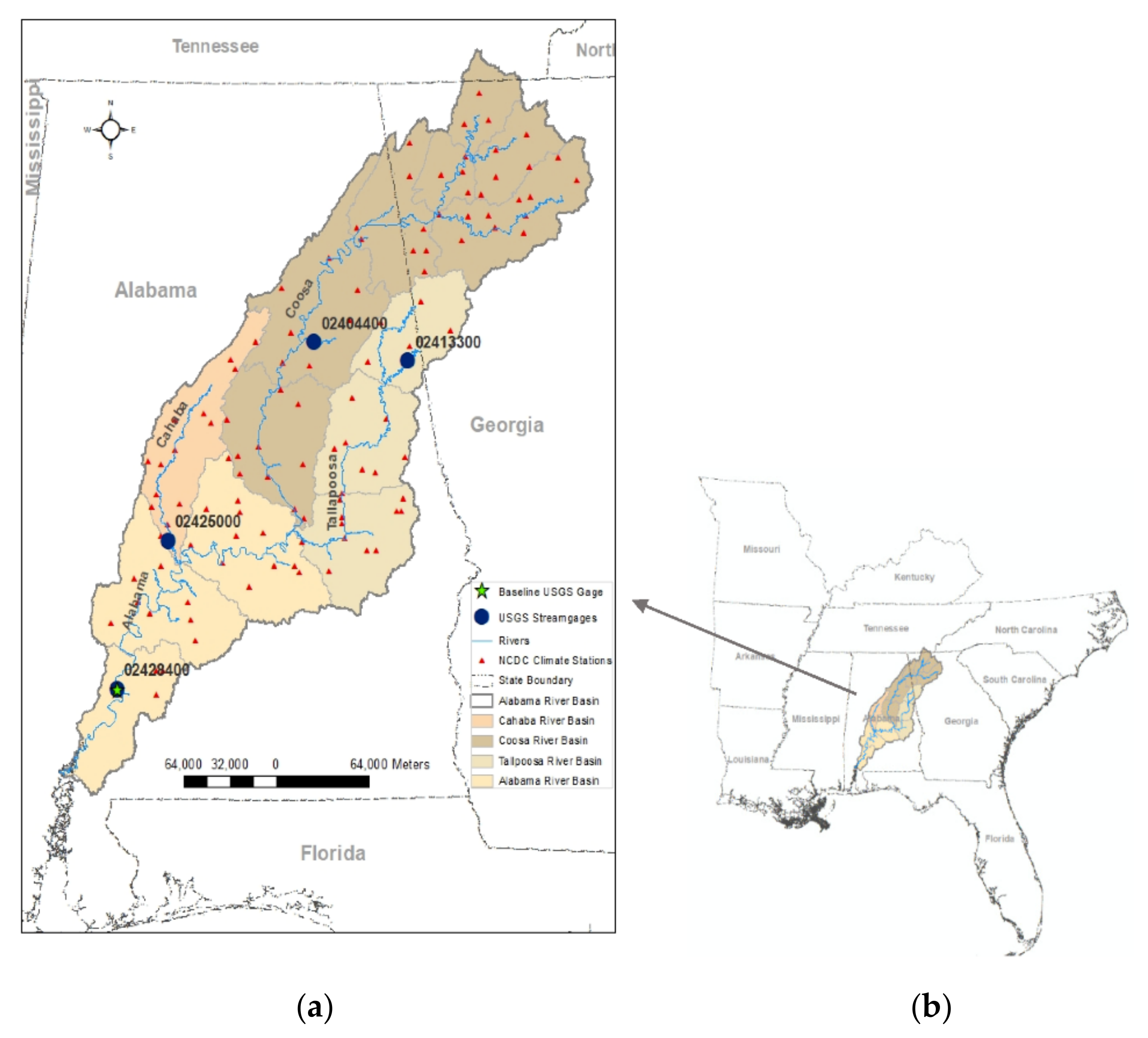
2.1. Study Area
2.2. Soil and Water Assessment Tool
2.3. General Circulation Models and Uncertainties
2.4. Historical and Future Climate Scenario Data
2.5. Hydrologic Modeling Data
2.6. SWAT Model Setup, Calibration, and Validation Analysis
2.7. Climate Trend Analysis
2.8. Analysis of Simulated Baseline versus Future Streamflow Discharge
3. Results and Discussion
3.1. Comparison of GCM Climate Variables with Observed Baseline Values
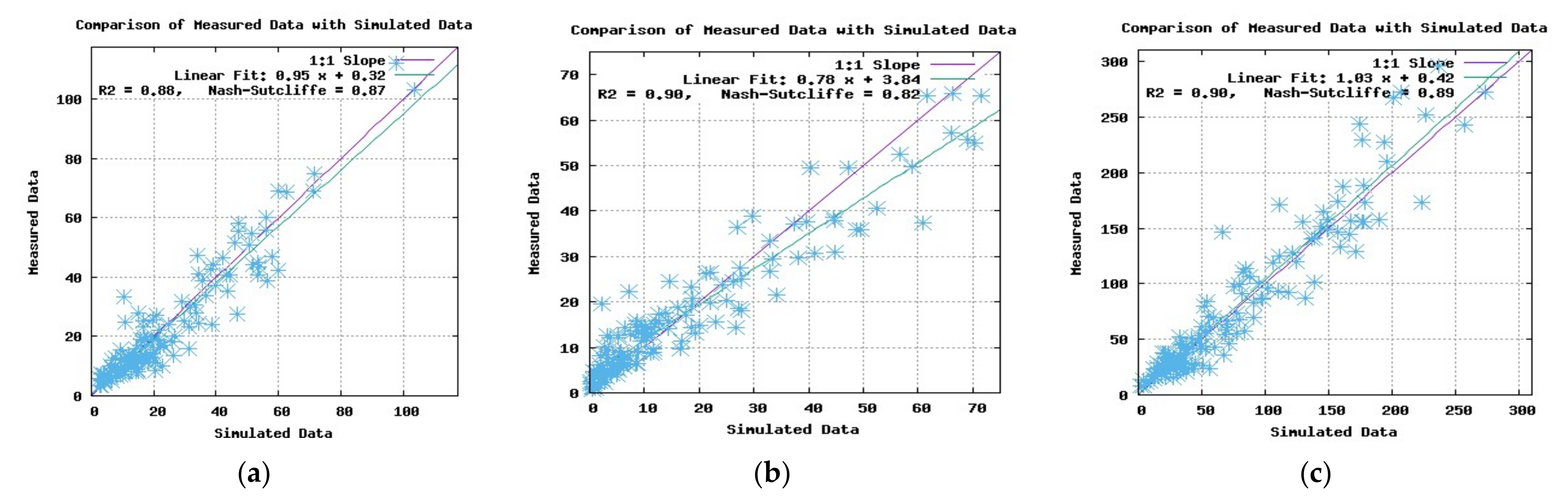
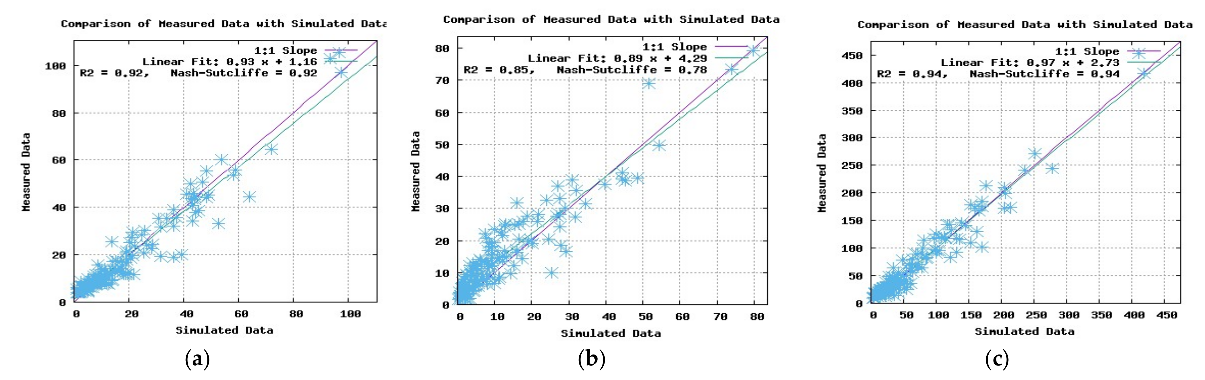
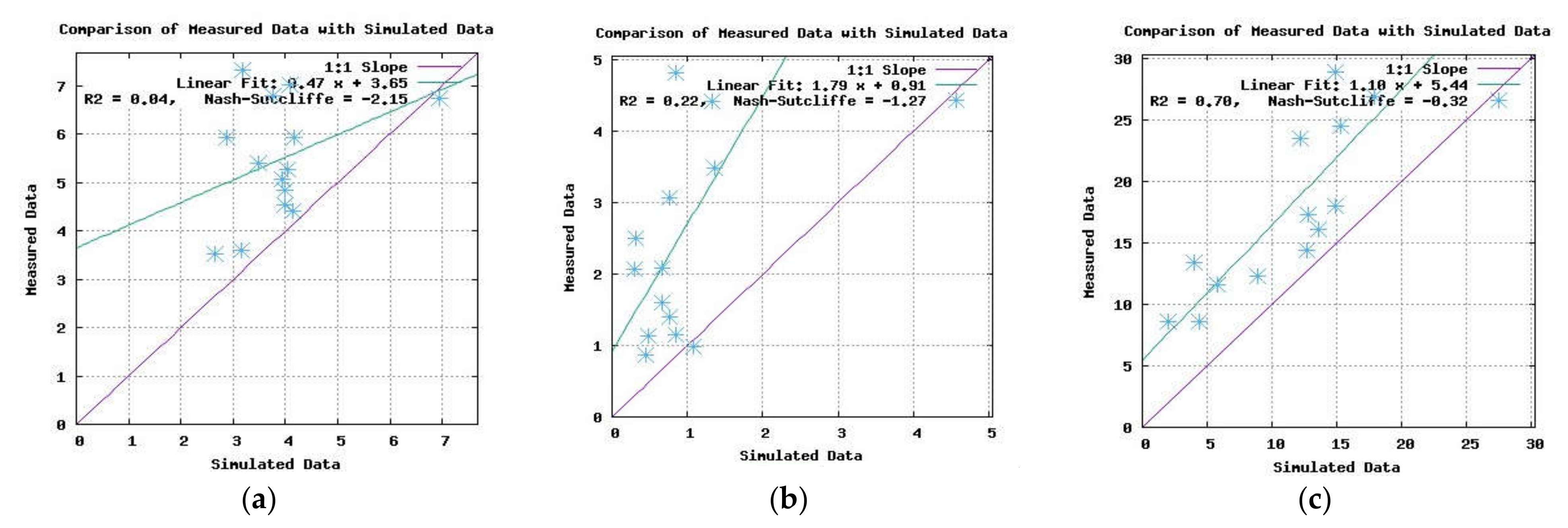
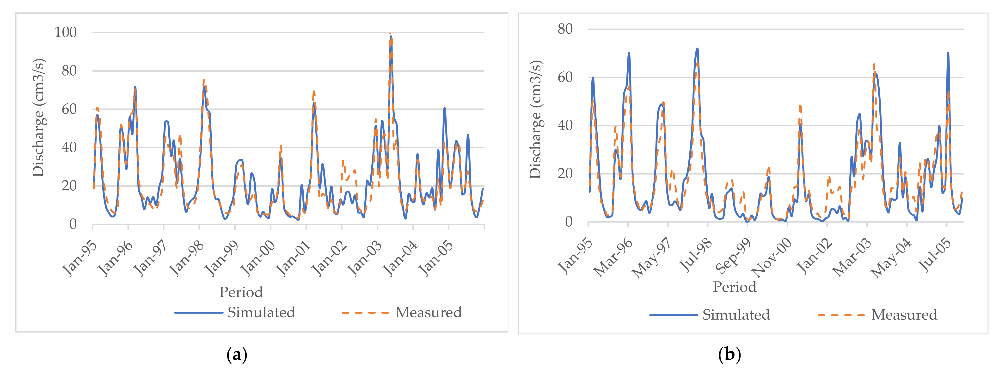
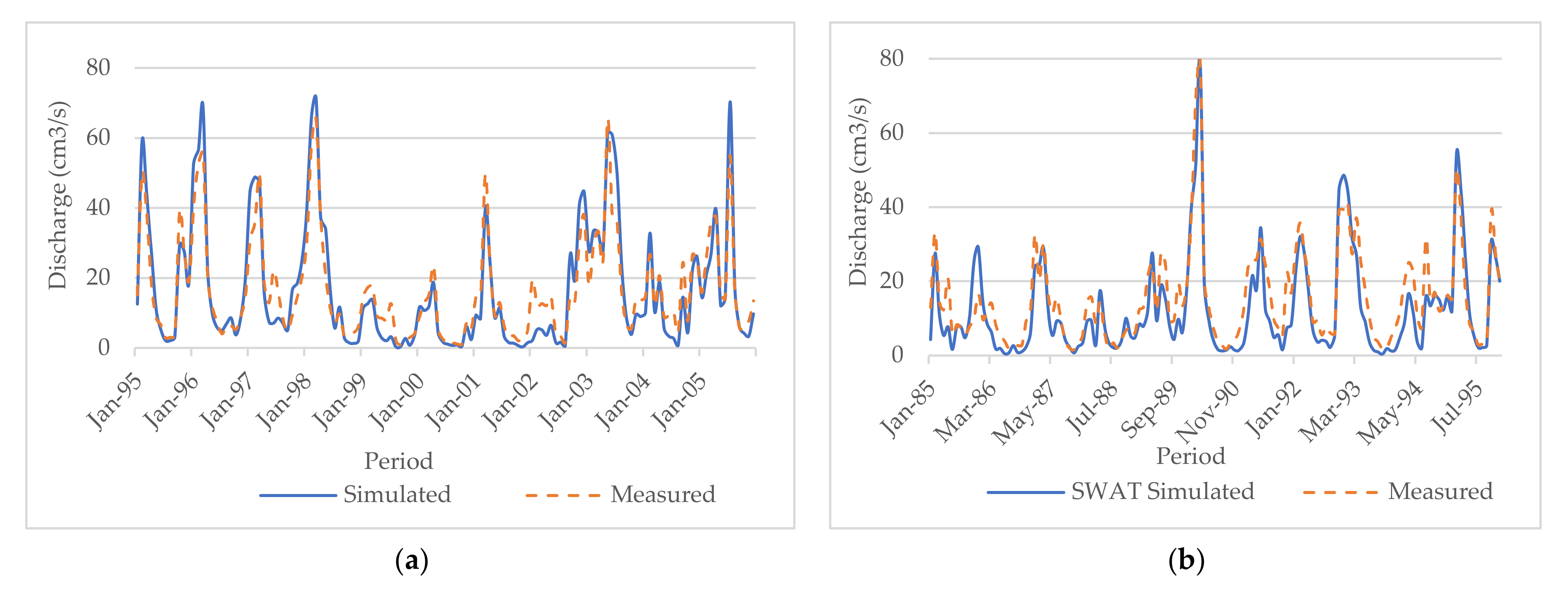
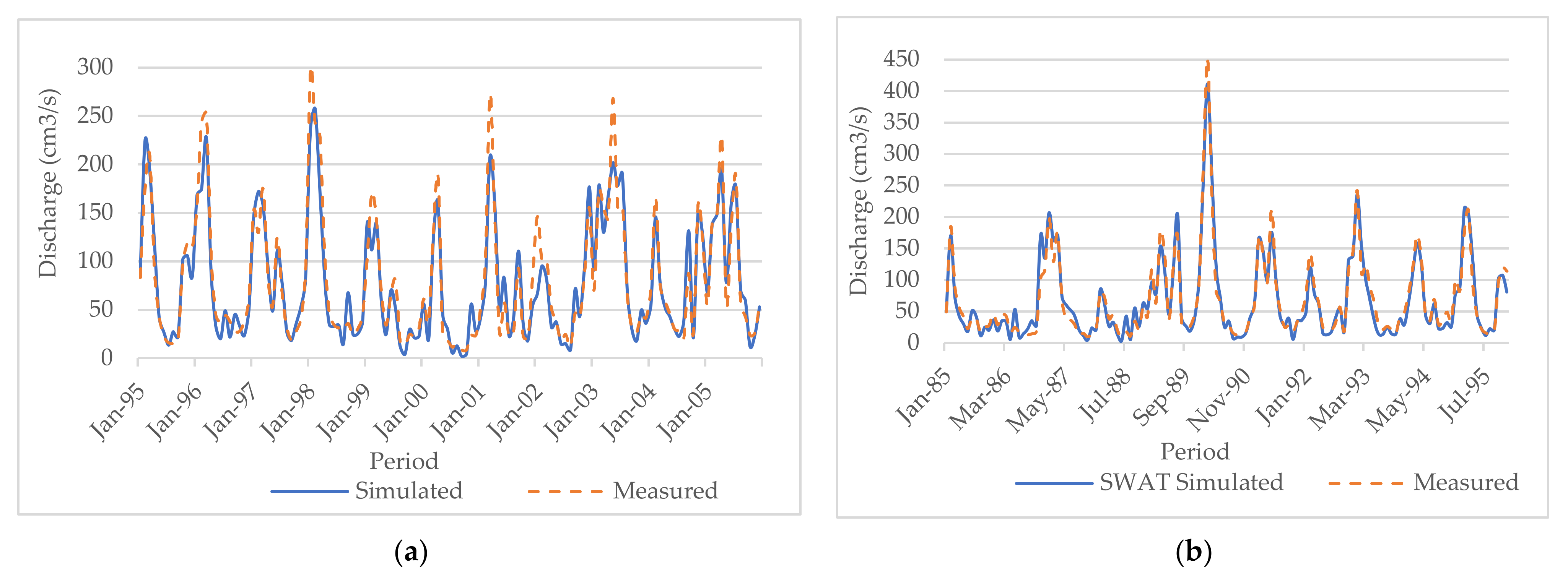
3.2. SWAT Model Calibration, Validation Results and Performance
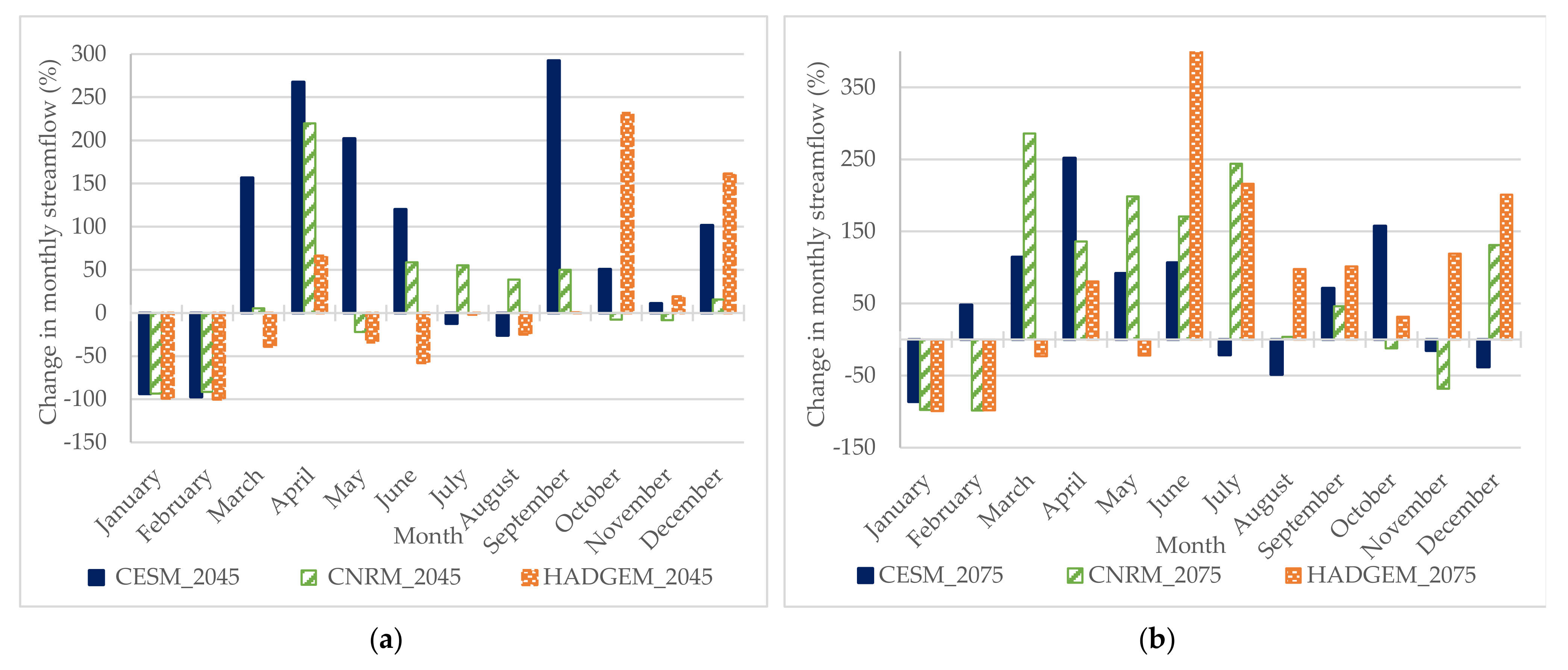
3.3. Analysis of Simulated Baseline against Future Streamflow
4. Conclusions
Author Contributions
Funding
Data Availability Statement
Acknowledgments
Conflicts of Interest
References
- UN General Assembly. United Nations Framework Convention on Climate Change (UNFCCC) (1992): Resolution Adopted by the General Assembly, 20 January 1994, A/RES/48/189. Available online: https://www.refworld.org/docid/3b00f2770.html (accessed on 12 June 2018).
- IPCC. Climate Change 2001: Synthesis Report. A Contribution of Working Groups I, II, and III to the Third Assessment Report of the Integovernmental Panel on Climate Change; Watson, R.T., the Core Writing Team, Eds.; Cambridge University Press: Cambridge, UK; New York, NY, USA, 2001; p. 398. [Google Scholar]
- IPCC. IPCC Special Report on Climate Change, Desertification, Land Degradation, Sustainable Land Management, Food Security, and Greenhouse Gas Fluxes in Terrestrial Ecosystems: Summary for Policymakers. 2019. Available online: https://www.ipcc.ch/site/assets/uploads/2019/08/4.-SPM_Approved_Microsite_FINAL.pdf (accessed on 5 April 2019).
- NASA. Scientific Consensus: Earth’s Climate is Warming. Available online: https://climate.nasa.gov/scientific-consensus/ (accessed on 19 November 2020).
- NASA Goddard Institute for Space Studies (GISS): Facts. 2020. Available online: https://climate.nasa.gov/vital-signs/global-temperature/ (accessed on 1 November 2020).
- Allen, M.R.; Dube, O.P.; Solecki, W.; Aragón-Durand, F.; Cramer, W.; Humphreys, S.; Kainuma, M.; Kala, J.; Mahowald, N.; Mulugetta, Y.; et al. Framing and Context. In Global Warming of 1.5 °C. An IPCC Special Report on the Impacts of Global Warming of 1.5 °C above Pre-Industrial Levels and Related Global Greenhouse Gas Emission pathways, in the Context of Strengthening the Global Response to the Threat of Climate Change, Sustainable Development, and Efforts to Eradicate Poverty; Masson-Delmotte, V., Zhai, P., Pörtner, H.-O., Roberts, D., Skea, J., Shukla, P.R., Pirani, A., Moufouma-Okia, W., Péan, C., Pidcock, R., et al., Eds.; The Intergovernmental Panel on Climate Change: Geneva, Switzerland, 2018. [Google Scholar]
- Seneviratne, S.I.; Nicholls, N.; Easterling, D.; Goodess, C.M.; Kanae, S.; Kossin, J.; Luo, Y.; Marengo, J.; McInnes, K.; Rahimi, M.; et al. Changes in climate extremes and their impacts on the natural physical environment. In Managing the Risks of Extreme Events and Disasters to Advance Climate Change Adaptation; Field, C.B.V., Barros, T.F., Stocker, D., Qin, D.J., Dokken, K.L., Ebi, M.D., Mastrandrea, K.J., Mach, G.-K., Plattner, S.K., Allen, M., Eds.; A Special Report of Working Groups I and II of the Intergovernmental Panel on Climate Change (IPCC); Cambridge University Press: Cambridge, UK; New York, NY, USA, 2012; pp. 109–230. [Google Scholar]
- IPCC. Climate Change Synthesis Report Summary Chapter for Policymakers; IPCC: Geneva, Switzerland, 2014. [Google Scholar]
- UNESCO. The impact of global change on water resources: The Response of UNESCO’s International Hydrologic Programme; Division of Water Sciences: Paris, France, 2011. Available online: https://unesdoc.unesco.org/ark:/48223/pf0000192216 (accessed on 5 December 2020).
- Bates, B.C.; Kundzewicz, Z.W.; Wu, S.; Palutikof, J.P. (Eds.) Climate Change and Water. Technical Paper of the Intergovernmental Panel on Climate Change; IPCC Secretariat: Geneva, Switzerland, 2008. [Google Scholar]
- Gleick, P.H. Water- The potential consequences of climate variability and change for the water resources of the United States. In The Report of the Water Sector Assessment Team of the National Assessment of the Potential Consequences of Climate Variability and Change for the U.S. Global Change Research Program; Peter, H.G., Ed.; Pacific Institute for Studies in Development, Environment, and Security: Oakland, CA, USA, 2000; pp. 126–151. ISBN 1-893790-04-5. [Google Scholar]
- U.S. Environmental Protection Agency (EPA). Climate Change Indicators in the United States, 4th ed.; EPA 430-R-16-004; 2016. Available online: www.epa.gov/climate-indicators (accessed on 20 May 2020).
- Weiskopf, S.R.; Rubenstein, M.A.; Crozier, L.G.; Gaichas, S.; Griffis, R.; Halofsky, J.E.; Hyde, K.J.W.; Morelli, T.L.; Morisette, J.T.; Muñoz, R.C.; et al. Climate change effects on biodiversity, ecosystems, ecosystem services, and natural resource management in the United States. Sci. Total Environ. 2000, 733. [Google Scholar] [CrossRef] [PubMed]
- Pitz, C.F. Predicted Impacts of Climate Change on Groundwater Resources of Washington State. Department of Ecology, The State of Washington. Report No. 16-03-006; 2016. Available online: https://fortress.wa.gov/ecy/publications/documents/1603006.pdf (accessed on 7 April 2019).
- Vincent, W.F. Effects of Climate Change on Lakes; Elsevier Inc.: Quebec City, QC, Canada, 2009; pp. 55–60. [Google Scholar]
- Lins, H.F. USGS Hydro-Climatic Data Network 2009 (HCDN-2009); U.S. Geological Survey Fact Sheet 2012-3047; U.S. Geological Survey: Reston, VA, USA, 2009. Available online: https://pubs.usgs.gov/fs/2012/3047/pdf/fs2012-3047.pdf (accessed on 8 June 2020).
- U.S. Geological Survey (USGS). Analysis of Data from the National Water Information System; U.S. Geological Survey (USGS): Reston, VA, USA, 2006.
- Hoegh-Guldberg, O.; Jacob, D.; Taylor, M.M.; Bindi, M.; Brown, S.; Camilloni, I.; Diedhiou, A.; Djalante, R.; Ebi, K.L.; Engelbrecht, F.; et al. Impacts of 1.5 °C global warming on natural and human systems. In Global Warming of 1.5 °C. An IPCC Special Report on the Impacts of Global Warming of 1.5 °C above Pre-Industrial Levels and Related Global Greenhouse Gas Emission Pathways, in the Context of Strengthening the Global Response to the Threat of Climate Change, Sustainable Development, and Efforts to Eradicate Poverty; Masson-Delmotte, V., Zhai, P., Pörtner, H.-O., Roberts, D., Skea, J., Shukla, P.R., Pirani, A., Moufouma-Okia, W., Péan, C., Pidcock, R., et al., Eds.; 2018; In Press. [Google Scholar]
- Ali, R.; Kuriqi, A.; Abubaker, S.; Kisi, O. Long-Term Trends and Seasonality Detection of the Observed Flow in Yangtze River Using Mann-Kendall and Sen’s Innovative Trend Method. Water 2019, 11, 1855. [Google Scholar] [CrossRef]
- Kuriqi, A.; Ali, R.; Pham, Q.B.; Gambini, J.M.; Gupta, V.; Malik, A.; Linh, N.T.T.; Joshi, Y.; Anh, D.T.; Dong, X.; et al. Seasonality shift and streamflow flow variability trends in central India. Acta Geophys. 2020, 68, 1461–1475. [Google Scholar] [CrossRef]
- Pathak, T.; Maskey, M.; Dahlberg, J.; Kearns, F.; Bali, K.; Zaccaria, D. Climate change trends and impacts on California agriculture: A detailed review. Agronomy 2018, 8, 25. [Google Scholar] [CrossRef]
- Mirzabaev, A.; Wu, J.; Evans, J.; García-Oliva, F.; Hussein, I.A.G.; Iqbal, M.H.; Kimutai, J.; Knowles, T.; Meza, F.; Nedjraoui, D.; et al. Desertification. In Climate Change and Land: An IPCC Special Report on Climate Change, Desertification, Land Degradation, Sustainable Land Management, Food Security, and Greenhouse Gas Fluxes in Terrestrial Ecosystems; Shukla, P.R., Skea, J., Calvo Buendia, E., Masson-Delmotte, V., Pörtner, H.-O., Roberts, D.C., Zhai, P., Slade, R., Connors, S., van Diemen, R., et al., Eds.; IPCC: Geneva, Switzerland, 2019. [Google Scholar]
- IPCC. Climate Change 2014: Synthesis Report Summary for Policymakers. Contribution of Working Groups I, II and III to the Fifth Assessment Report of the Intergovernmental Panel on Climate Change. Available online: https://www.ipcc.ch/site/assets/uploads/2018/02/AR5_SYR_FINAL_SPM.pdf (accessed on 12 August 2020).
- Randall, D.A.; Wood, R.A.; Bony, S.; Colman, R.; Fichefet, T.; Fyfe, J.; Kattsov, V.; Pitman, A.; Shukla, J.; Srinivasan, J.; et al. Climate Models and Their Evaluation; Cambridge University Press: Cambridge, UK, 2007. [Google Scholar]
- Alexander, L.V.; Arblaster, J.M. Historical and projected trends in temperature and precipitation extremes in Australia in observations and CMIP5. Weather Clim. Extremes 2017, 34–56. [Google Scholar] [CrossRef]
- Li, Z.; Jin, J. Evaluating climate change impacts on streamflow variability based on a multisite multivariate GCM downscaling method. Hydrol. Earth Syst. Sci. Discuss. 2017, 1–22. [Google Scholar] [CrossRef]
- Miao, C.; Duan, Q.; Sun, Q.; Huang, Y.; Kong, D.; Yang, T.; Gong, W. Assessment of CMIP5 climate models and projected temperature changes over Northern Eurasia. Environ. Res. Lett. 2004, 9. [Google Scholar] [CrossRef]
- Koch, J.; Cornelissen, T.; Fang, Z.; Bogena, H.; Diekkrüger, B.; Kollet, S.; Stisen, S. Inter-comparison of three distributed hydrological models with respect to seasonal variability of soil moisture patterns at a small forested catchment. J. Hydrol. 2016, 533, 234–249. [Google Scholar] [CrossRef]
- Leta, O.T.; El-Kadi, A.I.; Dulai, H.; Ghazal, K.A. Assessment of climate change impacts on water balance components of Heeia watershed in Hawaii. J. Hydrol. Reg. Stud. 2016, 8, 182–197. [Google Scholar] [CrossRef]
- Mohammed, I.N.; Bomblies, A.; Wemple, B.C. The use of CMIP5 data to simulate climate change impacts on flow regime within the Lake Champlain Basin. J. Hydrol. Reg. Stud. 2016, 3, 160–186. [Google Scholar] [CrossRef]
- Sunde, M.G.; He, H.S.; Hubbart, J.A.; Urban, M.A. Integrating downscaled CMIP5 data with a physically based hydrologic model to estimate potential climate change impacts on streamflow processes in a mixed-use watershed. Hydrol. Proc. 2017, 31, 1790–1803. [Google Scholar] [CrossRef]
- Su, B.; Huang, J.; Zeng, X.; Gao, C.; Jiang, T. Impacts of climate change on streamflow in the upper Yangtze River basin. Clim. Change 2017, 141, 533–546. [Google Scholar] [CrossRef]
- Kleinschmidt, E. Alabama River Basin Management Plan. 2005. Available online: http://www.adem.state.al.us/programs/water/nps/files/AlabamaBMP.pdf (accessed on 4 July 2020).
- Murgulet, D.G.; Tick, G. The extent of saltwater intrusion in southern Baldwin County, Alabama. Environ. Geol. 2008, 55, 1235–1245. [Google Scholar] [CrossRef]
- Sinclair, W.C. Sinkhole development resulting from ground water withdrawal in the Tampa Area, Florida. In USGS Water-Resources Investigations Report 81-50; 1982. Available online: https://pubs.usgs.gov/wri/1981/0050/report.pdf (accessed on 14 June 2020).
- Runkle, J.; Kunkel, K.; Stevens, L.; Frankson, R. Alabama State climate summary. In NOAA Technical Report NESDIS 149-AL; March 2019 Revision; Auburn University: Auburn, AL, USA, 2017; 4 pp. [Google Scholar]
- Karl, T.R.; Melillo, J.M.; Peterson, T.C. Global Climate Change Impacts in the United States. 2009; Volume 54. Available online: www.globalchange.gov/usimpacts (accessed on 12 August 2018).
- IPCC. Summary for Policymakersin: Managing the Risks of Extreme Events and Disasters to Advance Climate Change Adaptation; Field, C.B.V., Barros, T.F., Stocker, D., Qin, D.J., Dokken, K.L., Ebi, M.D., Mastrandrea, K.J., Mach, G.-K., Plattner, S.K., Allen, M., Eds.; A Special Report of Working Groups I and II of the Intergovernmental Panel on Climate Change; Cambridge University Press: Cambridge, UK; New York, NY, USA, 2012; pp. 14–15. [Google Scholar]
- U.S. Army Corps of Engineers (USACE). Environmental Data Inventory, State of Alabama: Mobile, Alabama; USACE: Washington, DC, USA, 1998. [Google Scholar]
- Gangrade, S.; Kao, S.-C.; McManamay, R.A. Multi-model Hydroclimate Projections for the Alabama-Coosa-Tallapoosa River Basin in the Southeastern United States. Nat. Res. Sci. Rep. 2020, 10. [Google Scholar] [CrossRef] [PubMed]
- Arnold, J.G.; Srinivasan, R.; Muttiah, R.S.; Williams, J.R. Large area hydrologic modeling and assessment part I: Model development. J. Am. Water Resour. Assoc. 1998, 34, 73–89. [Google Scholar] [CrossRef]
- Krysanova, V.; White, M. Advances in water resources assessment with SWAT—An overview. Hydrol. Sci. J. 2015, 60, 771–783. [Google Scholar] [CrossRef]
- Neitsch, S.L.; Arnold, J.G.; Kiniry, J.R.; Srinivasan, R.; Williams., J.R. Soil and Water Assessment Tool, User Manual, Version 2000; Grassland, Soil and Water Research Laboratory-Agricultural Research Service: Temple, TX, USA. Available online: https://swat.tamu.edu/media/1294/swatuserman.pdf (accessed on 8 January 2019).
- Bennett, J.C.; Grose, M.R.; Corney, S.P.; White, C.J.; Holz, G.K.; Katzfey, J.J.; Post, D.A.; Bindoff, N.L. Performance of an empirical bias-correction of a high-resolution climate dataset. Int. J. Climatol. 2014, 34, 2189–2204. [Google Scholar] [CrossRef]
- Aryal, Y.; Zhu, J. Multimodel ensemble projection of meteorological drought scenarios and connection with climate based on spectral analysis. Int. J. Climatol. 2020, 40, 3360–3379. [Google Scholar] [CrossRef]
- Zhao, T.; Dai, A. The magnitude and causes of global drought changes in the twenty-first century under a low–moderate emissions scenario. J. Clim. 2015, 28, 4490–4512. [Google Scholar] [CrossRef]
- Rupp, D.E. An evaluation of 20th century climate for the Southeastern United States as simulated by Coupled Model Intercomparison Project Phase 5 (CMIP5) global climate models. U.S. Geological Survey Open-File Report; U.S. Geological Survey: Reston, VA, USA, 2016; 32 p. [Google Scholar] [CrossRef]
- Voldoire, A.; Sanchez-Gomez, E.; Salas, D.; Mélia, Y.; Decharme, B.; Cassou, C.; Sénési, S.; Valcke, S.; Beau, I.; Alias, A.; et al. The CNRM-CM5.1 global climate model: Description and basic evaluation. Clim. Dyn. 2011, 40, 2091–2121. [Google Scholar] [CrossRef]
- Long, M.C.; Lindsay, K.S.; Peacock, S.; Moore, J.K.; Doney, S.C. Twentieth-Century Oceanic Carbon Uptake and Storage in CESM1(BGC). J. Clim. 2013, 26, 6775–6800. [Google Scholar] [CrossRef]
- Bellouin, N.; Collins, W.J.; Culverwell, I.D.; Halloran, P.R.; Hardiman, S.C.; Hinton, T.J.; Jones, C.D.; McDonald, R.E.; McLaren, A.J.; O’Connor, F.M.; et al. The HadGEM2 family of Met Office Unified Model climate configurations. Geosci. Model Devel. 2011, 4, 723–757. [Google Scholar]
- Thomson, A.M.; Calvin, K.V.; Smith, S.J.; Kyle, G.P.; Volke, A.; Patel, P.; Delgado-Arias, S.; Bond-Lamberty, B.; Wise, M.A.; Clarke, L.E.; et al. RCP4.5: A pathway for stabilization of radiative forcing by 2100. Clim. Chang. 2011, 109, 77. [Google Scholar] [CrossRef]
- Maurer, E.P. Uncertainty in hydrologic impacts of climate change in the Sierra Nevada, California under two emissions scenarios. Clim. Chang. 2007, 82, 309–325. [Google Scholar] [CrossRef]
- Quansah, J.E.; Engel, B.A.; Chaubey, I. Tillage Practices Usage in Early Warning Prediction of Atrazine Pollution. Transac. ASABE 2008, 51, 1311–1321. [Google Scholar] [CrossRef][Green Version]
- Arnold, J.G.; Moriasi, D.N.; Gassman, P.W.; Abbaspour, K.C.; White, M.J.; Srinivasan, R.; Santhi, C.; Harmel, R.D.; van Griensven, A.; Van Liew, N.W.; et al. SWAT: Model use, calibration, and validation. Trans. ASABE 2012, 55, 1491–1508. [Google Scholar] [CrossRef]
- Nash, J.E.; Sutcliffe, J.V. River flow forecasting through conceptual models: Part 1. A discussion of principles. J. Hydrol. 1970, 10, 282–290. [Google Scholar] [CrossRef]
- Moriasi, D.N.; Arnold, J.G.; Van Liew, M.W.; Bingner, R.L.; Harmel, R.D.; Veith, T.L. Model evaluation guidelines for systematic quantification of accuracy in watershed simulations. Trans. ASABE 2007, 50, 885–900. [Google Scholar] [CrossRef]
- Krause, P.; Boyle, D.P.; Base, F. Comparison of different efficiency criteria for hydrological model assessment. Adv. Geosci. 2005, 5, 89–97. [Google Scholar] [CrossRef]
- McCuen, R.H. Assessment of Hydrological and statistical significance. J. Hydrol. Eng. ASCE 2016, 21. [Google Scholar] [CrossRef]
- Mann, H.B. Nonparametric tests against trend. Econometrica 1945, 13, 245–259. [Google Scholar] [CrossRef]
- Sen, P. Estimated of the regression coefficient based on Kendall’s Tau. J. Am. Stat. Assoc. 1968, 39, 1379–1389. [Google Scholar] [CrossRef]
- Theil, H. A rank-invariant method of linear and polynomial regression analysis, I, II, III. In Henri Theil’s Contributions to Economics and Econometrics; Volume 23, Springer: Dordrecht, The Netherlands, 1992. [Google Scholar] [CrossRef]
- Parra, V.; Arumí, J.L.; Muñoz, E. Identifying a Suitable Model for Low-Flow Simulation in Watersheds of South-Central Chile: A Study Based on a Sensitivity Analysis. Water 2019, 11, 1506. [Google Scholar] [CrossRef]
- Garcia, F.; Folton, N.; Oudin, L. Which objective function to calibrate rainfall–runoff models for low-flow index simulations? Hydrol. Sci. J. 2017. [Google Scholar] [CrossRef]


| Data | Data Source | Data Description |
|---|---|---|
| Elevation (30 m) | United States Department of Agriculture Geospatial Data Gateway http://datagateway.nrcs.usda.gov | National Elevation Dataset |
| State Soil Geographic data | United Stated Department of Agriculture Geospatial Data Gateway http://datagateway.nrcs.usda.gov | Soil classification and properties |
| Land Use (30 m) | United Stated Department of Agriculture Geospatial Data Gateway http://datagateway.nrcs.usda.gov | National Land Cover Dataset Land |
| Historical Climate | National Climatic Data Center http://www.ncdc.noaa.gov/cdo-web | Daily rainfall, maximum and minimum temperature |
| Streamflow | United States Geological Survey Water Data https://waterdata.usgs.gov/nwis | Monthly streamflow |
| Future Climate | http://gdo-dcp.ucllnl.org/downscaled_cmip_projections/ | Downscaled General Circulation Model data for 2045 and 2075 |
| Variable | Number of Years | Mann–Kendall | Trend |
|---|---|---|---|
| Precipitation | 30 | + | 1 |
| Maximum Temperature | 30 | + | 0 |
| Minimum Temperature | 30 | + | 1 |
| Climate Data Type | Precipitation (mm/day) | Precipitation Change (%) | Maximum Temperature (°C) | Maximum Temperature Change (%) | Minimum Temperature (°C) | Minimum Temperature Change (%) |
|---|---|---|---|---|---|---|
| Baseline_1980 | 3.93 | 24.42 | 10.69 | |||
| CNRM-CM5_2045 | 3.62 | −7.89 | 24.29 | −0.53 | 11.33 | 5.99 |
| CESM1-BGC.1_2045 | 3.99 | 1.53 | 27.42 | 12.29 | 14.75 | 37.98 |
| HADGEM2-AO.1_2045 | 3.91 | −0.509 | 26.89 | 10.11 | 13.46 | 25.91 |
| CNRM-CM5_2075 | 3.63 | −7.63 | 24.3 | −0.49 | 11.32 | 5.89 |
| CESM1-BGC.1_2075 | 3.99 | 1.53 | 26.47 | 8.39 | 13.25 | 23.95 |
| HADGEM2-AO.1_2075 | 4.48 | 13.99 | 27.98 | 14.58 | 14.62 | 36.76 |
| Streamflow Calibration | Component Variables | Description of Variables | Default Value | Calibrated Value | Input File |
|---|---|---|---|---|---|
| Surface | CN2 | SCS runoff curve number for moisture condition II | 27–94 | Reduced by 4 for all sub-basins | .mgt |
| ESCO | Soil evaporation compensation factor | 0.95 | 0.90 | .bsn | |
| SOL_AWC | Soil available water capacity | 0–0.35 | Increased by 0.2 | .sol | |
| Baseflow | ALPHA_BF | Groundwater recession factor | 0.048d | replaced with 0.3 | .gw |
| GW_REVAP | Groundwater revap coefficient | 0.02 | increased by 0.1 | .gw | |
| GWQMIN | Threshold depth of water in the shallow aquifer required for return flow to occur | 1000 | 800 | .gw |
| Station Location | USGS Gage No. | Drainage Area (km2) | Calibration | Validation | ||
|---|---|---|---|---|---|---|
| R2 | NSE | R2 | NSE | |||
| Choccolocco Creek at Jackson Shoal near Lincoln | 2404400 | 1245 | 0.88 | 0.87 | 0.92 | 0.92 |
| Little Tallapoosa River near Newell | 2413300 | 1050 | 0.90 | 0.82 | 0.85 | 0.78 |
| Cahaba River near Marion Junction | 2425000 | 4567 | 0.90 | 0.89 | 0.94 | 0.94 |
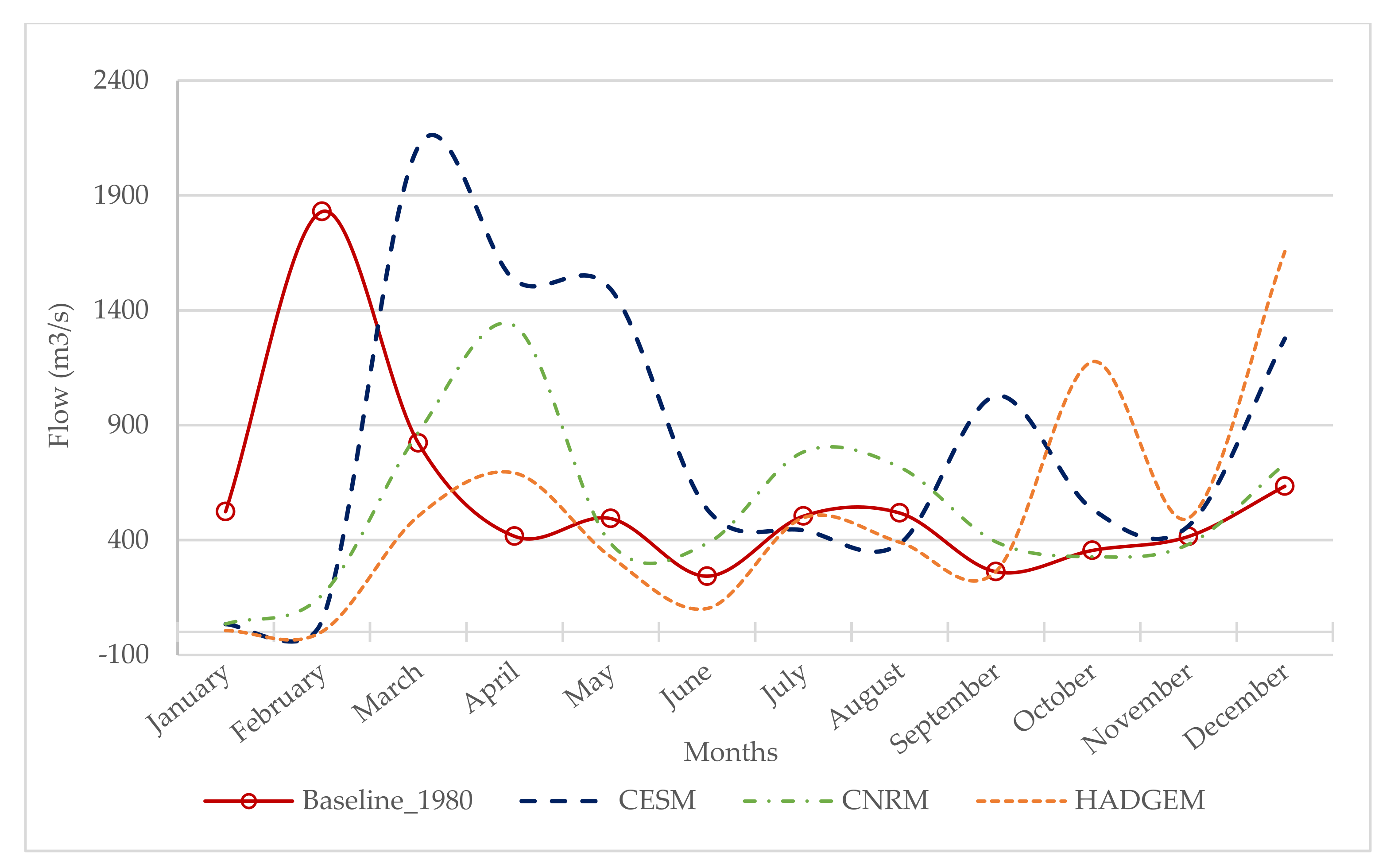
| Months | Baseline | CESM (m3/s) | CNRM (m3/s) | HADGEM (m3/s) |
|---|---|---|---|---|
| January | 523.58 | 33.61 | 35.15 | 6.19 |
| February | 1829.83 | 48.65 | 160.30 | 1.39 |
| March | 823.17 | 2112.00 | 867.90 | 504.60 |
| April | 416.82 | 1532.00 | 1333.00 | 692.00 |
| May | 493.85 | 1491.00 | 385.10 | 327.20 |
| June | 242.73 | 534.40 | 385.40 | 102.40 |
| July | 504.61 | 443.00 | 783.30 | 497.20 |
| August | 517.92 | 384.50 | 717.70 | 390.80 |
| September | 261.99 | 1028.00 | 392.90 | 262.90 |
| October | 354.82 | 534.90 | 328.10 | 1176.00 |
| November | 415.98 | 461.90 | 381.40 | 495.20 |
| December | 634.01 | 1277.00 | 731.80 | 1656.00 |
| Average | 584.94 | 823.41 | 541.84 | 509.32 |
| Percentage change to 1980 baseline | 40.77 | −7.37 | −12.93 | |
| Correlation between baseline and GCMs | −0.18 | −0.20 | −0.22 | |
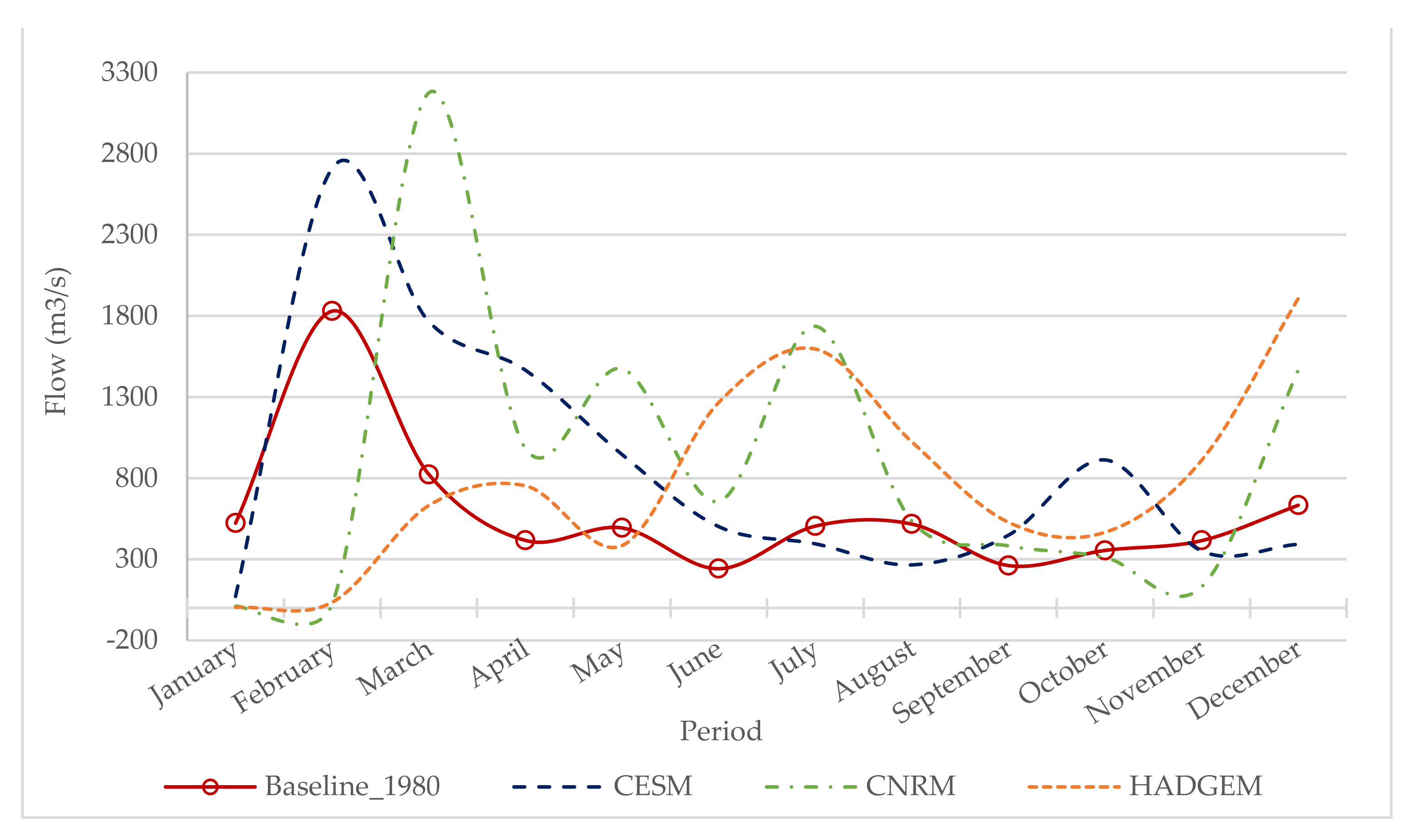
| Months | 1980 Baseline | CESM (m3/s) | CNRM (m3/s) | HADGEM (m3/s) |
|---|---|---|---|---|
| January | 523.58 | 71.79 | 11.42 | 4.73 |
| February | 1829.83 | 2710.00 | 25.84 | 35.61 |
| March | 823.17 | 1765.00 | 3176.00 | 632.00 |
| April | 416.82 | 1466.00 | 983.60 | 753.20 |
| May | 493.85 | 946.00 | 1474.00 | 384.80 |
| June | 242.73 | 501.70 | 657.00 | 1266.00 |
| July | 504.61 | 396.40 | 1736.00 | 1596.00 |
| August | 517.92 | 266.40 | 536.40 | 1024.00 |
| September | 261.99 | 448.30 | 382.80 | 528.40 |
| October | 354.81 | 913.10 | 311.50 | 466.80 |
| November | 415.98 | 351.40 | 132.10 | 911.20 |
| December | 634.01 | 392.50 | 1466.00 | 1908.00 |
| Average | 584.94 | 852.38 | 907.72 | 792.56 |
| Percentage change to 1980 Baseline | 45.72 | 55.18 | 35.49 | |
| Correlation between baseline and GCMs | 0.79 | −0.01 | −0.35 | |
Publisher’s Note: MDPI stays neutral with regard to jurisdictional claims in published maps and institutional affiliations. |
© 2021 by the authors. Licensee MDPI, Basel, Switzerland. This article is an open access article distributed under the terms and conditions of the Creative Commons Attribution (CC BY) license (https://creativecommons.org/licenses/by/4.0/).
Share and Cite
Quansah, J.E.; Naliaka, A.B.; Fall, S.; Ankumah, R.; Afandi, G.E. Assessing Future Impacts of Climate Change on Streamflow within the Alabama River Basin. Climate 2021, 9, 55. https://doi.org/10.3390/cli9040055
Quansah JE, Naliaka AB, Fall S, Ankumah R, Afandi GE. Assessing Future Impacts of Climate Change on Streamflow within the Alabama River Basin. Climate. 2021; 9(4):55. https://doi.org/10.3390/cli9040055
Chicago/Turabian StyleQuansah, Joseph E., Amina B. Naliaka, Souleymane Fall, Ramble Ankumah, and Gamal El Afandi. 2021. "Assessing Future Impacts of Climate Change on Streamflow within the Alabama River Basin" Climate 9, no. 4: 55. https://doi.org/10.3390/cli9040055
APA StyleQuansah, J. E., Naliaka, A. B., Fall, S., Ankumah, R., & Afandi, G. E. (2021). Assessing Future Impacts of Climate Change on Streamflow within the Alabama River Basin. Climate, 9(4), 55. https://doi.org/10.3390/cli9040055