Article

Impact of Climate Variability on Crop Yield in Kalahandi, Bolangir, and Koraput Districts of Odisha, India

1
Department of Geography, Delhi School of Economics, University of Delhi, Delhi 110007, India
2
Disaster Prevention Research Institute, Kyoto University, Kyoto 606-8501, Japan
3
Application Laboratory, JAMSTEC, Kanagawa 2360001, Japan
4
Department of Environmental Science, Fakir Mohan University, Odisha 756019, India
5
Faculty of Environment Earth Science, Hokkaido University, Sapporo 060-0810, Japan
*
Author to whom correspondence should be addressed.
Climate 2019, 7(11), 126; https://doi.org/10.3390/cli7110126
Submission received: 2 September 2019 / Revised: 2 October 2019 / Accepted: 3 October 2019 / Published: 28 October 2019

Abstract

:
Most tropical regions in the world are vulnerable to climate variability, given their dependence on rain-fed agricultural production and limited adaptive capacity owing to socio-economic conditions. The Kalahandi, Bolangir, and Koraput districts of the south-western part of Odisha province of India experience an extreme sub-humid tropical climate. Based on the observed changes in the magnitude and distribution of rainfall and temperature, this study evaluates the potential impact of climate variation on agricultural yield and production in these districts. The study is conducted by taking into account meteorological data like rainfall and temperature from 1980 to 2017 and crop productivity data from 1980–81 to 2016–17. Additionally, climate variability indices like Monsoon Index, Oceanic Nino Index, and NINO-3 and NINO 3.4 are used. To analyse the data, various statistical techniques like correlation and multiple linear regression are used. The amount of monsoon rainfall is found to have a significant impact on crop productivity, compared to temperature, in the study area, and as a result the Monsoon Index has a determining impact on crop yield among various indices.

1. Introduction

Climate is one of the main factors for agricultural production and yield. Climate parameters, mainly rainfall and temperature [1,2,3], directly affect cultivation, and any change in them is bound to have a significant impact on crop yield and production. There is a growing concern all over the world about the effects of climate variability [4,5] on agricultural production. Several studies have already shown the considerable impact of variations [6,7] in climate parameters [8,9] on the average crop yield [10,11,12]. Most of the agricultural crops and, specifically, the kharif season crops are sensitive to their growing conditions, especially rainfall and temperature, which consequently come under the key factors influenced by climate variation. Kharif crops are usually sown with the beginning of the first rains during the advent of the south-west monsoon season, and they are harvested at the end of monsoon season (October–November). These crops are dependent on the quantity of rain water as well its timing. El Nino affects the flow of moisture-bearing winds from the cooler oceans towards India, and negatively affects the summer monsoon, i.e., the south-west monsoon, which accounts for over 70% of annual rainfall; therefore, El Nino conditions play a significant role in affecting summer monsoon, which in turn affects the crop yield. Hence, rainfall and temperature deviation [13,14,15] from season to season greatly affects soil water availability to crops and thus poses crop production risks. It is easy to comprehend such annual variation, in a changing climate [16,17] that could affect crop production [18] and growth.
Odisha, a poor and underdeveloped state with a substantial amount of under-privileged people (nearly 40 percent SC and ST population) [19] and a backward subsistence-oriented agricultural economy, has failed to bridge the development disparities that have long existed between the people and the state at the inter-district level. In recent years, three of the old and undivided backward districts, namely, Kalahandi, Bolangir, and Koraput (hereafter KBK), in the southwestern part of Odisha, have become vulnerable to recurring droughts and famine-like situations, which have led to distress migration of the poor during the non-agricultural season. The KBK districts of Odisha comprise one of the poorest regions of the state with most of the population living Below the Poverty Line (BPL); out of the total working population, 30.60 per cent are cultivators and 48.75 are agricultural labourers [19]. Furthermore, the frequent recurrence of drought and flood has created situations like starvation, epidemics, and mass migration in these districts. However, instability in agricultural production is on the rise due to several factors such as erratic rainfall pattern [20], low irrigation coverage, and an increase in the frequency and severity of natural disasters, among others. Therefore, the present study attempts to measure the agricultural productivity in the above mentioned districts and makes an attempt to analyze the nature of the relationship between agricultural productivity and climatic parameters in the studied districts of western Odisha.

2. Study Area

The districts of southern and western Odisha, re-designated KBK [13] (Kalahandi, Bolangir and, Koraput) districts (Figure 1), are regarded as the most backward region in the state by the planning commission. The district Kalahandi occupies the south-western portion of Odisha and is situated between 19°3′ N to 21°5′ N latitudes and 82°20′ E to 83°47′ E longitudes. It extends over an area of 11,835 sq kms. and ranks fourth among the districts of Odisha with regard to its size. Koraput is the southernmost district of Odisha and is situated between 17°50′ N to 20°30′ N latitude and 81°27′ E to 84°10′ E longitude. Bolangir is situated on 20°67′ N latitude and 83°16′ E longitude. It is a district situated in the western region of Odisha and has an area of 5165 km2.

3. Data Sources and Methodology

3.1. Data Sources

The present study is based on meteorological data collected for Bhawanipatna station (Kalahandi district), Bolangir station (Bolangir district), and Koraput station (Koraput district), having the Index numbers 43042, 42963, and 42097, respectively, observed by the India Meteorological Department (IMD). The data was described and summarized quantitatively and qualitatively. In this study, the selected meteorological stations that had no missing data. Available historical climate data on rainfall and temperature of western Odisha, of three districts, covered a period of 38 years from 1980 to 2017. Meteorological stations were selected based on the availability of daily rainfall data, minimum temperature data, and maximum temperature data in the study area. Data pertaining to area, yield, and production (AYP) of crops, landholding pattern, irrigation, fertilizer consumption, rainfall, etc., were collected for Bolangir, Kalahandi, and Koraput, as a whole, from the Directorate of Economics and Statistics, Department of Planning, Directorate of Agriculture and Food Production, Government of Odisha, Bhubaneswar. Crops/crop groups selected for the study were rice and maize. The study covers a period of 37 years: 1980–1981 to 2016–2017.

3.2. Methodology

Two staple crops, Rice and Maize, are selected for analysis, since they cover maximum cultivation area and are the major sources of livelihood. It is important here to note that the year to year crop yield, area, and rainfall variations (y’) are defined as anomalous percentage deviated from the five year running mean to stress the anomalies related to climatic variations as shown in Equation (1), i.e.,
y’ = [(y − y’’)/y’’] * 100
where
  • y: annual crop yield/ area/ rainfall
  • y’: anomaly of the variables like crop yield, rainfall, temperature
  • y’’: five year running mean
Based on this calculation, deficient yield years are derived and relationship between rainfall as well as temperature deviation and crop yield is established for those deficient years and for both the crops. Regression analysis is used for the exploration of relationships among rainfall, temperature, and crop yield and production [21]. The investigators seek to determine the influence of one variable upon another leading to certain causalities, as in this case analysis of the effect of temperature and rainfall deviation upon different crop productions. Regression analysis is used to assess the quantitative effect of the underlying variables upon the dependent variable—the variable that is influenced. Furthermore, the statistical significance of the approximate relationships is then determined. A simple regression is illustrated in the following (Equation (2)) formula:
I =α + β E + ε
  • α = constant
  • β = effect/coefficient
  • I = dependent
  • E = exogenous
Within this formula there are observable as well as unobservable variables [21]. I and E are observable variables, since they are available from collected data. On the contrary, α, β are unobservable parameters and ε a random term. The purpose of regression analysis is then to produce an estimate for these three parameters based on the data set. The example above is of a linear nature, which is common in regression analysis.
Coming back to the formula expressed above, in order to understand the relationship between I and E, their role in generating the noise, ε, is ignored for a while. Graphically, the relationship between I and E constitutes the equation for a line where β is the slope and α the intercept on the vertical axis. Integrating the noise ε suggests that there can be numerous lines depending on the range of ε. Further, a particular regression line relates to the estimated noise term, based on the error for each observation. For each probable line, a set of errors will result, and among the possible lines, the regression analysis will select the “sum of the squares of the estimated errors at a minimum”, the so-called “minimum sum of squarederrors (SSE)”.
Furthermore, multiple regression is a technical tool permitting to quantify the impact of several synchronized influences upon a specific dependent variable [21]. The expression for a multiple regression formula results (Equation (3)) in
I = α + βE + γX + ε
for example, where γ is expected to be positive. The coefficients α, β, and γ remain to be estimated. In addition, the SSE will depend upon the particular value of ε, in this case crop, within the data set. Moreover, the regression properties involve the relationship among the true values of the parameters and the probability distribution of those parameter estimates. Each parameter estimate that is produced by an estimator is defined as a random variable constrained from a selected probability distribution. If the mean of the probability distribution in question is equivalent to the true value of the parameter, that is to be estimated, the estimator will remain unbiased. In other terms, if the estimator is unbiased, on average, the true value of each parameter will be recovered.

3.3. Climatic Indices

Various climate indices like Monsoon Index (hereafter MI), Oceanic Nino Index (hereafter ONI), and NINO-3 have been used in the study to examine the climate variability impact on crops. Among various monsoon indices, “Indian Summer Monsoon Index”, based on zonal wind, is used, which is computed using NCEP-NCAR reanalysis, as follows (Equation (4)):
MI Index = U850 (40° E–80° E, 5° N–15° N) − U850 (70° E–90° E, 20° N–30° N)
means difference between U850 (zonal wind at 850 mb) over two regions with varied latitudinal and longitudinal extension, as mentioned in Equation (1) [22]. MI is an indicator of Indian Summer Monsoon rainfall, which is defined by the seasonally averaged precipitation over all the Indian sub divisions from June to September. The MI not only represents the rainfall anomalies averaged over an extended region, including the Bay of Bengal, India, and the eastern Arabian Sea, it is also highly correlated with the all-India summer rainfall, and this has a great impact on Indian kharif cropping pattern.
ONI, believed to have strong impact on rainfall [23,24], is one of NOAA’s primary indices for monitoring the relative strength of El Niño/ Southern Oscillation (ENSO). Its cycle is related to strong anomalous warming/cooling condition in eastern tropical pacific and cooling/warming condition in western tropical pacific. It is calculated by taking three month running average derived from ERSST.V4 (Extended Reconstruction SST. Version 4) SST anomalies for the Nino 3.4 (5° N–5° S, 120° W–170° W) region. The impact of El Nino–southern oscillation (ENSO) on the Indian monsoon rainfall is well known. The authors of [25] have shown a statistically significant positive correlation between the Indian monsoon rainfall and sea-surface temperatures (SSTs) over most parts of the north Indian Ocean at lead times of 6–12 months. Hence, the potential (associated with ENSO and other large-scale climate teleconnections) to anticipate fluctuations in both monsoon rainfall and resulting agricultural production prior to the start of the growing season has important implications for agricultural decision making at farm and policy levels.
Nino 3 index is calculated by taking area average of SST anomalies in °C (degrees Celsius) of region over eastern Pacific Ocean, which is bounded by 90°W–150°W and 5°S–5°N.
Purposive sampling techniques were used in the selection of study site and sample households. Criteria considered for the selection of study area were representativeness, prevalence of the problem, availability of relevant data, and proximity to meteorology station. In order for the study to be reliable, 150 interviewees were carefully selected within the three districts. In addition, it was preferred that the selected interviewees in question had more than five years of experience within the agricultural production domain and were full-time farmers. In our analyses of the results of primary survey, the number of respondents has been converted to percentage.

4. Results and Discussion

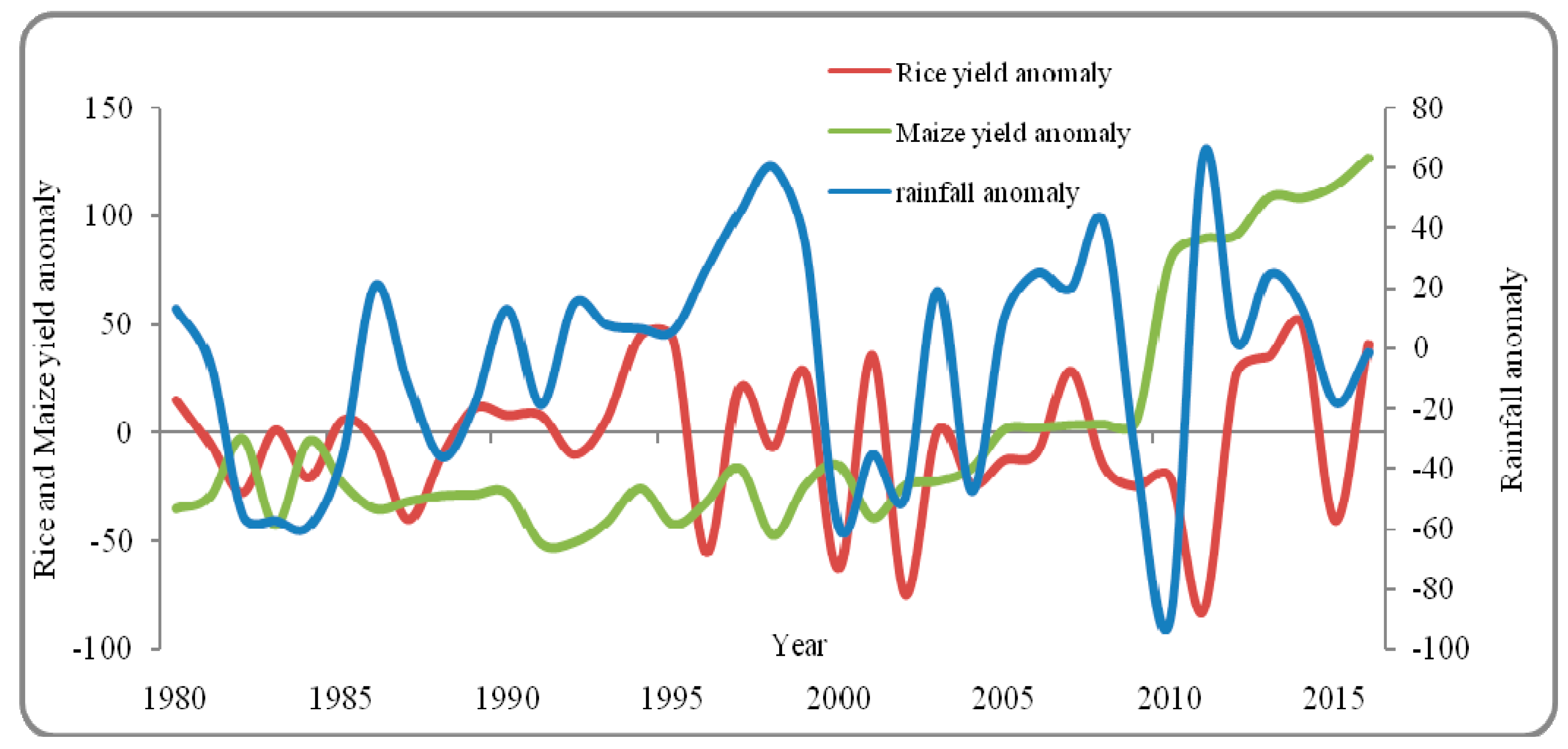
Climate variability [26,27,28] and change have emerged as the most prominent global issues, and there is a need to evaluate their impact on vulnerable socio-economic sectors such as agriculture. Additionally, understanding the regional manifestations of recent climate trends can help us to prepare for future climatic effects on agricultural productivity. Among the various parameters of climatic variability [29], rainfall [30] and temperature [31,32] play the most determining roles [33,34] in defining agricultural conditions. This is also true for the districts being studied here. The location map of the study area and its soil types are shown in Figure 1 and Figure 2, respectively. Figure 2 shows the relationship between rainfall anomaly and rice and maize yield anomaly. Furthermore, it can be seen from the figure that both are generally following a direct relationship, i.e., when one increases (i.e., the independent variable rainfall), the other ones also increase (i.e., dependent variables rice and maize yield anomaly) and vice versa.
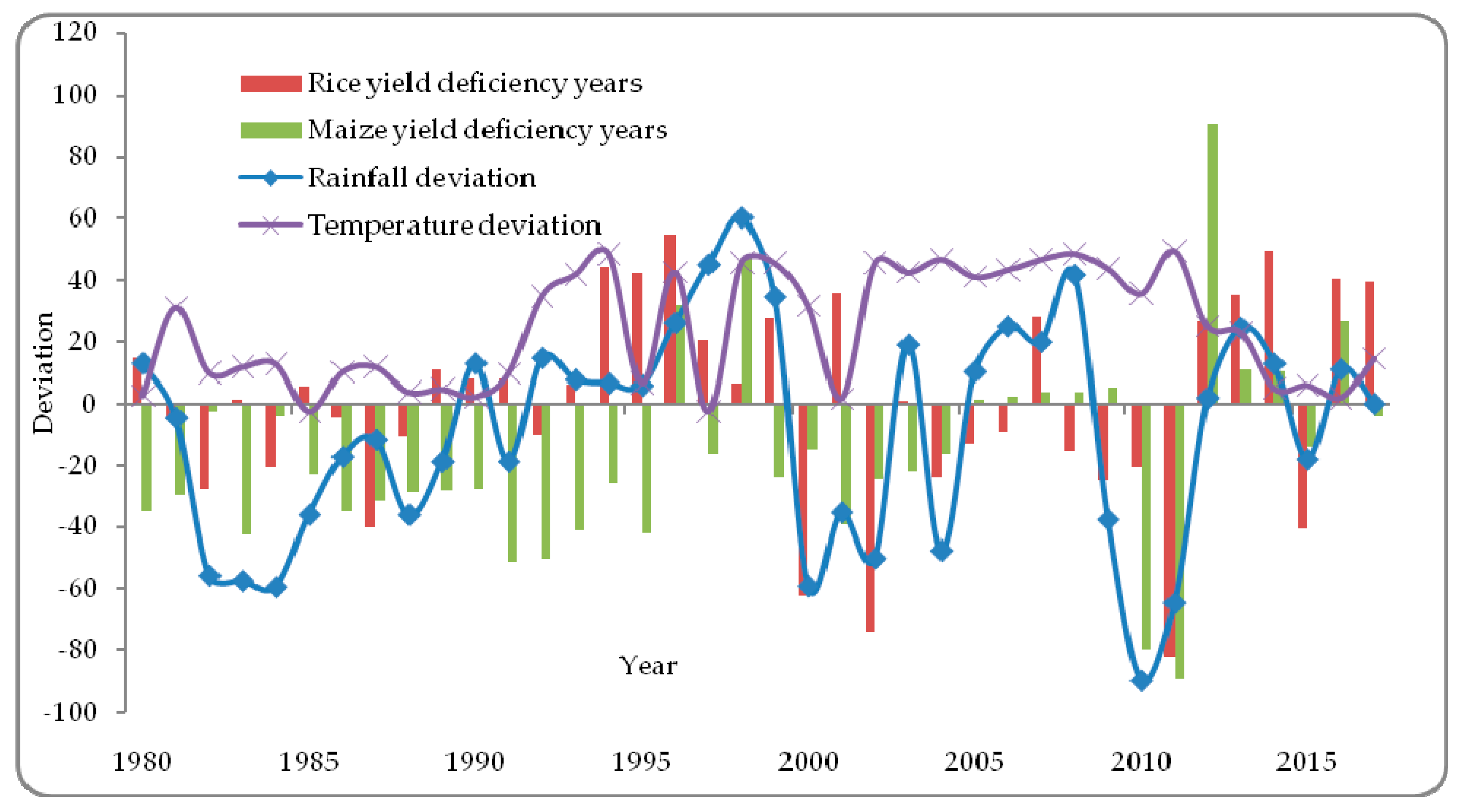
Rainfall deviation years as well as temperature deviation years with more than 10% of the mean have been calculated and compared with the maize and rice yields for Niño/ deficient years. Figure 3 gives a clear visual representation of rainfall deviation years, negatively, and temperature deviation years, positively, of above 10% of the mean, along with crop yield deficiency years. It is found that the rainfall deviation years result in reductions in rice and maize yields (Table 1). Similarly, when there is increase in temperature by more than 10% of the mean, this results in the deficiency of rice and maize yields. Though the amount varies, rainfall deviation has a higher impact compared to that of the temperature. For example, as shown in Table 1, in the year 1981 rainfall deviation is −25.44%, and the rice yield for the year 1981–1982 is −33.11 %. Similar results can be seen for maize yield, like in the year 1982, when the temperature increase is 31.22% and maize yield is −23.12%.
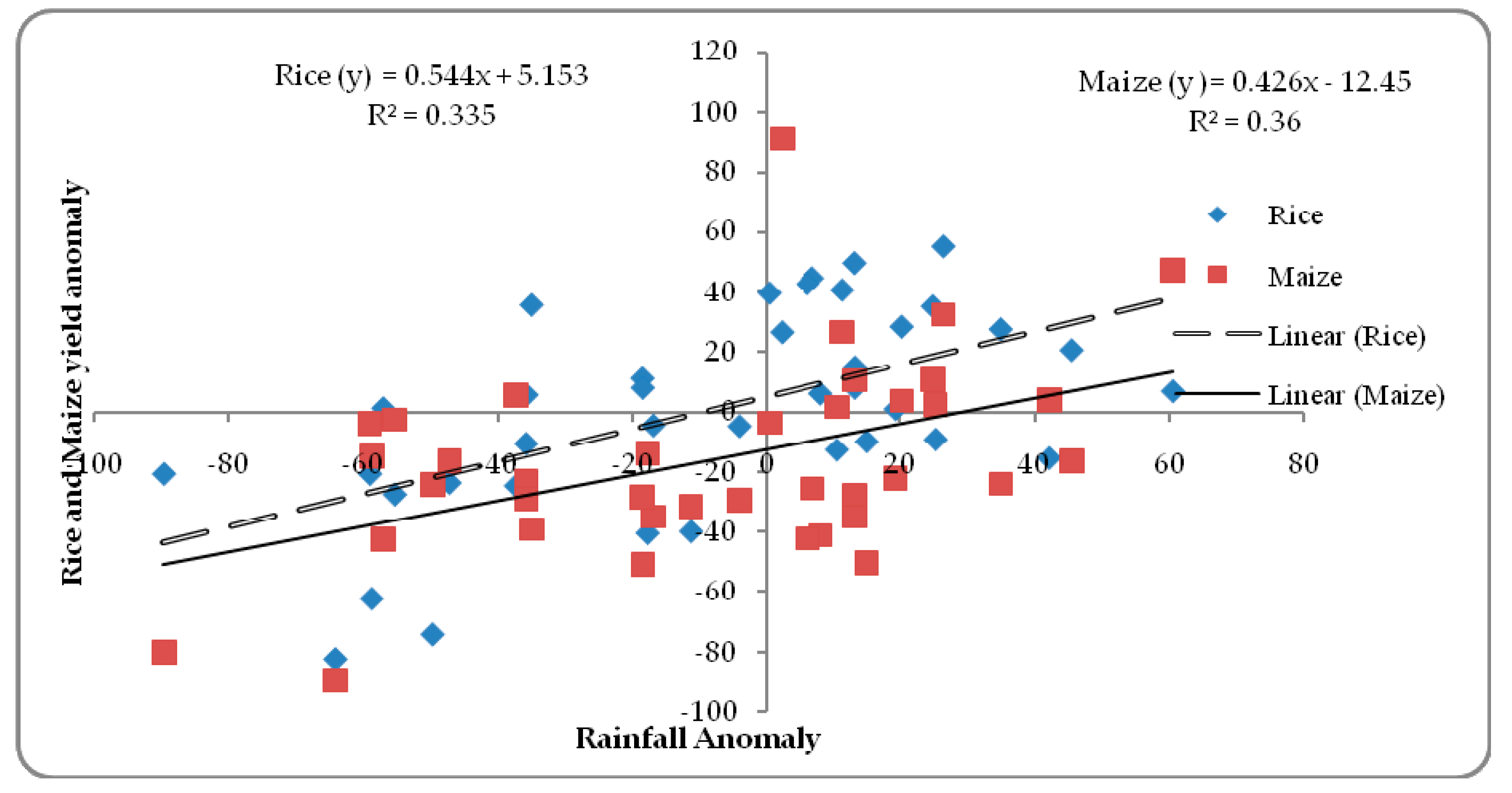
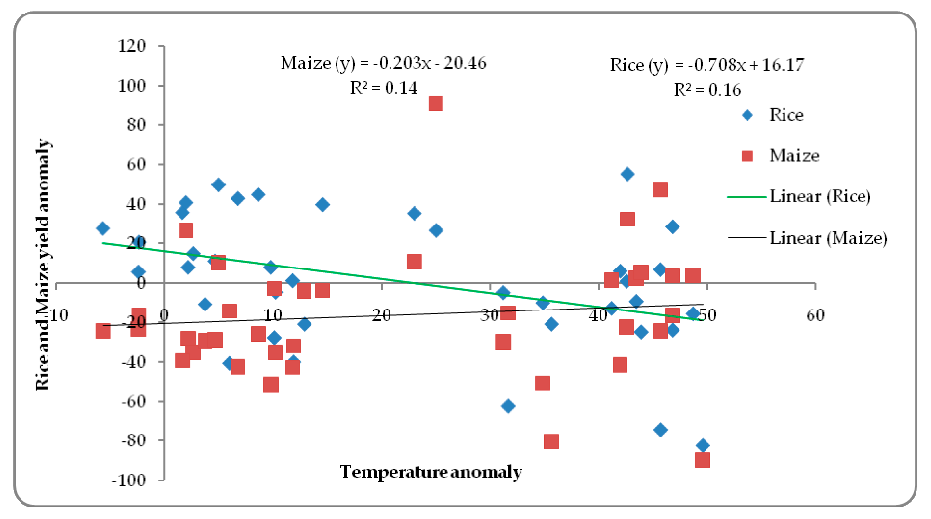
The correlations of rice and maize yield anomaly with rainfall and temperature anomaly suggest both the crops have negative relationship with temperature anomaly, i.e., −0.4 for rice and −0.38 for maize (Figure 4 and Figure 5). The correlation values with temperature anomaly are modest compared to positive correlation values for rainfall, i.e., 0.65 for rice yield and 0.6 for maize yield. Hence, the rainfall anomaly plays a decisive role in determining the crop yield.
Table 2 shows multiple linear regression analysis result where dependent variables are rice and maize yield anomalies, and independent variables are temperature and rainfall anomalies. The results show that rainfall anomaly plays a more significant role than temperature anomaly in determining rice and maize yield. The results are statistically significant at 0.018 (p value) for rice yield and 0.044 (p value) for maize yield. Ninety-five percent or 0.05 threshold value has been set for this analysis. Additionally, the R square value, which is the co-efficient of determination for rice yield, i.e., 0.732, and 0.544 for maize yield, makes the analysis much more significant. In other words, it can be said that 73% and 54% variations in rice and maize yield, respectively, can be predicted by one unit change in rainfall anomaly. However, the result of temperature anomaly for prediction of rice and maize yield was not significant and hence is not discussed further.
Monsoon plays a pivotal role in defining the rainfall pattern over the study region, which ultimately affects the crop productivity pattern. The region receives heavy rainfall during monsoon season of June to September, when the monsoon winds are the strongest. Therefore, the crop yield anomalies, with 5-year running mean, are correlated with the Monsoon Index for JJA, JAS, and JJAS seasons (Table 3). The Pearson’s Product Moment correlation coefficient was also calculated to study the variability impact. Important thing to mention here is that the correlation is calculated for the two crops separately. Furthermore, as the result shows, both rice and maize yield have strong positive relation with MI, i.e., 0.61, 0.66 for rice yield for MI-JJA and MI-JAS, respectively. After the correlation was computed with different seasonal Monsoon Indices, a multiple linear regression was carried on to identify the significance of seasonal Monsoon Index. As per the results shown in Table 4, Monsoon Indices of JJA and JJAS seasons play determining role in the prediction of crop yield in the study area; also, the statistical test is significant as the significance values are within the limit of 95% confidence level.
Other than the Indian monsoon, the study also attempts to understand the impact of Indo-Pacific climate variations, because it is well known that the Indo-Pacific climate variability largely influences regional phenomena such as Indian monsoon on a large scale. It can be said that the strength of Indian Monsoon, whether strong or weak, largely depends on the nature of Indo-Pacific climate variability [23]. Therefore, the relationship between rainfall and climate variation is very important, since the latter has a direct influence on Monsoon as well as on rainfall variability. To further elucidate the extent of the impact of the modes of Indo-Pacific climate variations, correlation analyses are carried out for crop yield anomalies with ONI, NINO-3.4, and NINO3 index of NDJ (November–January), DJF (December–February), and JFM (January-March) seasons (Table 5). It is noteworthy to mention here that the correlation [18] is calculated between crop yield anomaly of event specific years and ONI, NINO 3.4, and NINO3 index of NDJ (November, December month of previous year, and January month of event years); DJF (December month of previous year, January and February months of event year); and JFM (all three months are from event years), since ENSO phenomena in Pacific Ocean is in its peak occurrence during these time periods, i.e., November–March of one year only. Hence, to show the impact of an El Niño or La Niña event on rainfall pattern in the study area, correlation has been calculated for winter months. From the correlation table, it can be noticed that the Pacific climate variability indices affect the monsoon and, in turn, the agricultural yield or the cropping pattern, but as the correlation values shown in the table are moderate, so it can be said that due to time lag between the occurrence of Pacific climatic modes of variability and Indian summer rainfall, the effect is more or less moderate.
The interviewees’ perceptions of climate variables such as temperature and rainfall behavior of the area in past have been investigated through primary surveys. The results revealed that a higher proportion of farmers are of the opinion that both temperature and rainfall have been experiencing deviations and there has been a great change over the pattern of occurrence; also, they note extreme weather change particularly in the frequency of floods and droughts. Results show that almost 100% of the respondents perceived that rainfall has changed in their area in the last 20 years. Local communities have been experiencing fluctuations in rainfall and change in timing of rainfall over the past 20 years. Most of respondents believe in change of timing of rainfall, i.e., 70%, 60%, and 50% in Bolangir, Kalahandi, and Koraput, respectively. In this study, local people are also asked to tell what indicators they have been using to perceive changes in rainfall over the last 20 years. Their responses reveal that “decline of agricultural yields”, “rainfall comes early or lately”, “loss of some animal and plant species”, “decreased availability of water”, and “increased drought and flood frequency” to be the main indicators. Maximum respondents perceive “decline in crop yield” to be the major indicator for the change in rainfall trend. Thirty percent in Bolangir, 30% in Kalahandi, and 25% in Koraput reveal the arrival time of rainfall, i.e., the change in timing of rainfall, to be the second major reason for decline in crop yield.

5. Conclusions

This study draws upon quantitative and scientific approaches to investigate the climate variation impact on crop yield by analyzing meteorological data, i.e., rainfall and temperature, as well as climate variability indices, i.e., MI, ONI, and NINO 3. Mainly, the study establishes evidence of climate variability impact in the study area through an analysis of historical meteorological data from over the past 38 years. The agricultural practices in the three districts studied here are mainly rain-fed and are hence highly dependent on rainfall patterns. Among two studied climatic parameters (rainfall and temperature), rainfall is shown to have a tremendous impact on the yield of both staple crops under consideration (rice and maize). Again, among both the crops, the impact of rainfall on rice yield is seen to be higher than that of the impact on maize yield. MI, which is the main determinant of summer rainfall in the study area, is the main driving force behind high crop yield. Other climate indices like ONI and NINO 3 are shown to have a moderate impact on the crop yield of the study area; this may be due to the time lag between sowing season (May–June) of the crops and peak occurrence (November–December) of the climatic conditions in Pacific Ocean. Therefore, the study results reveal that deficit rainfall related to climate variations has a negative impact on the crop yield and livelihoods of smallholder subsistence farmers. Hence, proper and timely predictions of the climatic conditions could yield good results in the study area and some adaptive mechanisms could be taken on the basis of this to cope with the climatic extremities.

Author Contributions

Conceptualization, N.S. and S.B.; Data curation, A.P. and L.S.; Formal analysis, A.P. and N.S.; Methodology, A.P.; Supervision, N.S.; Visualization, L.S., R.A. and M.Y.; Writing—original draft, A.P.; Writing—review & editing, S.B., T.S., R.A., R.B.S.

Funding

This research received no external funding.

Acknowledgments

We are thankful to the India Meteorological Department, Pune, for providing required data used in this research article and for their effective response. We acknowledge software like ArcGIS, R used for making graphs in this article for their free downloading and availability of tutorials. We also acknowledge the library and computer centre facilities of University of Delhi for their prompt responses and available facilities. At present, Netrananda Sahu is working as JSPS Postdoc Fellow at DPRI, Kyoto University. We are thankful to JSPS (ID No. P18360), Japan.

Conflicts of Interest

There is no conflict of interest as per the authors.

References

  1. Asseng, S.; Cammarano, D.; Anothai, J.; Sanctis, G. Rising Temperatures reduce global Wheat Production. Nat. Clim. Chang. 2015, 5, 143–147. [Google Scholar] [CrossRef]
  2. De-Graft, H.A.; Kyei, C.K. The Effects of Climatic Variables and Crop Area on Maize Yield and Variability in Ghana. Russ. J. Agric. Socio-Econ. Sci. 2012, 10, 10–13. [Google Scholar]
  3. Dinar, A.; Mendelsohn, R.; Evenson, R.; Parikh, J.; Sanghi, A.; Kumar, K.; McKinsey, J.; Lonergan, S. Measuring the Impact of Climate Change on Indian Agriculture; Technical Report; The World Bank: Washington, DC, USA, 1998. [Google Scholar]
  4. Sahu, N.; Yamashiki, Y.; Behera, S.; Takara, K.; Yamagata, T. Large Impacts of Indo-Pacific Climate Modes on the Extremes Streamflows of Citarum River in Indonesia. J. Glob. Environ. Eng. 2012, 17, 1–8. [Google Scholar]
  5. Sahu, N.; Behera, S.; Yamashiki, Y.; Takara, K.; Yamagata, T. IOD and ENSO Impacts on the Extreme Streamflows of Citarum river in Indonesia. Clim. Dyn. 2012, 39, 1673–1680. [Google Scholar] [CrossRef]
  6. Egbebiyi, T.S.; Lennard, C.; Crespo, O.; Mukwenha, P.; Lawal, S.; Quagraine, K. Assessing Future Spatio-Temporal Changes in Crop Suitability and Planting Season over West Africa: Using the Concept of Crop-Climate Departure. Climate 2019, 7, 102. [Google Scholar] [CrossRef]
  7. Egbebiyi, T.S.; Crespo, O.; Lennard, C. Defining Crop-climate Departure in West Africa: Improved Understanding of the Timing of Future Changes in Crop Suitability. Climate 2019, 7, 101. [Google Scholar] [CrossRef]
  8. De Jager, J.M.; Schulze, R.E. The Broad Geographic Distribution in Natal of Climatological Factors important to Agricultural Planning. Agrochemophysica 1977, 9, 81–91. [Google Scholar]
  9. Deressa, T. Analysis of Perception and Adaptation to Climate Change in the Nile Basin of Ethiopia. J. Agric. Sci. 2008, 149, 23–31. [Google Scholar] [CrossRef]
  10. Fisher, G.; Shah, M.; Tubiello, F.; Helhuizen, H. Socio-economic and Climate Change impacts on Agriculture: An Integrated Assessment, 1990–2080. Philos. Trans. R. Soc. B 2005, 360, 2067–2083. [Google Scholar] [CrossRef] [PubMed]
  11. Gbetiobouo, G.A.; Hassan, R.M. Economic Impact of Climate Change on Major South African Field Crops: A Ricardian Approach. MSc Thesis, Faculty of Natural and Agricultural Sciences, University of Pretoria, Pretoria, South Africa, 2004. [Google Scholar]
  12. Gbetiobouo, G.A.; Hassan, R.M. Measuring the Economic Impact of Climate Change on Major South African Field Crops: A Ricardian Approach. Glob. Planet. Chang. 2004, 47, 143–152. [Google Scholar] [CrossRef]
  13. Panda, A.; Sahu, N. Trend Analysis of Seasonal Rainfall and Temperature Pattern in Kalahandi, Bolangir and Koraput Districts of Odisha, India. Atmos. Sci. Lett. 2019. [Google Scholar] [CrossRef]
  14. Seo, N.; Mendelsohn, R. A Ricardian Analysis of the Impact of Climate Change on South American Farms. Chil. J. Agric. Res. 2008, 68, 69–79. [Google Scholar] [Green Version]
  15. Loua, T.R.; Bencherif, H.; Mbatha, N.; Begue, N.; Hauchecorne, A.; Bamba, Z.; Sivakumar, V. Study on Temporal Variationsb of Surface Temperature and Rainfall at Conakry Airport, Guinea: 1960–2016. Climate 2019, 7, 93. [Google Scholar] [CrossRef]
  16. Iizumi, T.; Ramankutty, N. Changes in Yield Variability of Major Crops for 1981–2010 explained by climate change. Environ. Res. Lett. 2016, 11, 034003. [Google Scholar] [CrossRef]
  17. Cline, W.R. Global Warming and Agriculture: Impact Estimates by Country; Institute of International Economics: Washington, DC, USA, 2007. [Google Scholar]
  18. Hansen, J.W.; Jones, J.W. El Nino-Southern Oscillation Impacts on Winter Vegetable Production in Florida. J. Clim. 1999, 12, 92–102. [Google Scholar] [CrossRef]
  19. Census of India. Registrar General & Census Commsisioner, New Delhi. 2011. Available online: http://censusindia.gov.in/2011-Common/CensusData2011.html (accessed on 27 July 2019).
  20. Kumar, K.K.; Kumar, K.R.; Ashrit, R.G.; Deshpande, N.R.; Hansen, J.W. Climate Impacts on Indian Agriculture. Int. J. Climatol. 2004, 24, 1375–1393. [Google Scholar] [CrossRef]
  21. Keat, P.; Young, P. Managerial Economics, Economic Tools for Today’s Decision Makers, 3rd ed.; Prentice Hall: Upper Saddle River, NJ, USA, 2000; ISBN 0-13-013538-0. [Google Scholar]
  22. Wang, B.; Fan, Z. Choice of South Asian Summer Monsoon Indices. Bull. Amer. Meteor. Soc. 1999, 80, 629–638. [Google Scholar] [CrossRef] [Green Version]
  23. Rajeevan, M.; Azad, S. Possible shift in the ENSO- Indian monsoon rainfall relationship under future global warming. Sci. Rep. 2016, 6, 20145. [Google Scholar]
  24. Yuan, C.; Yamagata, T. Impacts of IOD, ENSO and ENSO Modoki on the Australian Winter Wheat Yields in Recent Decades. Sci. Rep. 2015, 5, 17252. [Google Scholar] [CrossRef]
  25. Clark, C.O.; Cole, J.E.; Webster, P.J. Indian Ocean SST and Indian summer rainfall: Predictive relationships and their decadal variability. J. Clim. 2000, 13, 2503–2519. [Google Scholar] [CrossRef]
  26. Sahu, N.; Singh, R.B.; Kumar, P.; Silva, V.D.; Behera, S. La Nina Imapcts on Austral Summer Extremely High-Streamflow Events of the Paranaiba River in Brazil. Adv. Meteorol. 2013. [Google Scholar] [CrossRef]
  27. Sahu, N.; Singh, R.B.; Duan, W.; Silva, V.D.; Behera, S.; Ratnam, J.V. El Nino Modoki Connection to Extremely-low Streamflow of the Paranaiba river in Brazil. Clim. Dyn. 2014, 42, 1509–1516. [Google Scholar] [CrossRef]
  28. Sahu, N.; Singh, R.B.; Kumar, M.; Behera, S.; Takara, K. Probabilistic Seasonal Streamflow Forecats of the Citarum river, Indonesia, based on General Circulation Models. Stoch. Environ. Res. Risk Assess. 2016. [Google Scholar] [CrossRef]
  29. Pandey, V.; Sharma, A.; Bharati, L.; Joshi, I.; Dhaubanjar, S. Climate Shocks and Responses in Karnali- Mahakali Basins, Western Nepal. Climate 2019, 7, 92. [Google Scholar] [CrossRef]
  30. Meshram, S.G.; Singh, S.K.; Meshram, C.; Deo, R.C.; Ambade, B. Statistical evaluation of rainfall time series in concurrence with agriculture and water resources of Ken River basin, Central India (1901–2010). Theor. Appl. Climatol. 2018, 134, 1231–1243. [Google Scholar] [CrossRef]
  31. Nayak, S.; Mandal, M. Impact of land use and land cover changes on temperature trends over western India. Curr. Sci. 2012, 102, 1166–1173. [Google Scholar]
  32. Nayak, S.; Mandal, M. Examining the impact of regional land use and land cover changes on temperature: The case of Eastern India. Spat. Inf. Res. 2019. [Google Scholar] [CrossRef]
  33. Schelenker, W.; Lobell, B.D. Robust Negative Impacts of Climate Change on African Agriculture. Environ. Res. Lett. 2010, 5. [Google Scholar] [CrossRef]
  34. Morton, J.F. The Impact of Climate Change on Smallholder and Subsistence Agriculture. Proc. Natl. Acad. Sci. USA 2007, 104, 19680–19685. [Google Scholar] [CrossRef]
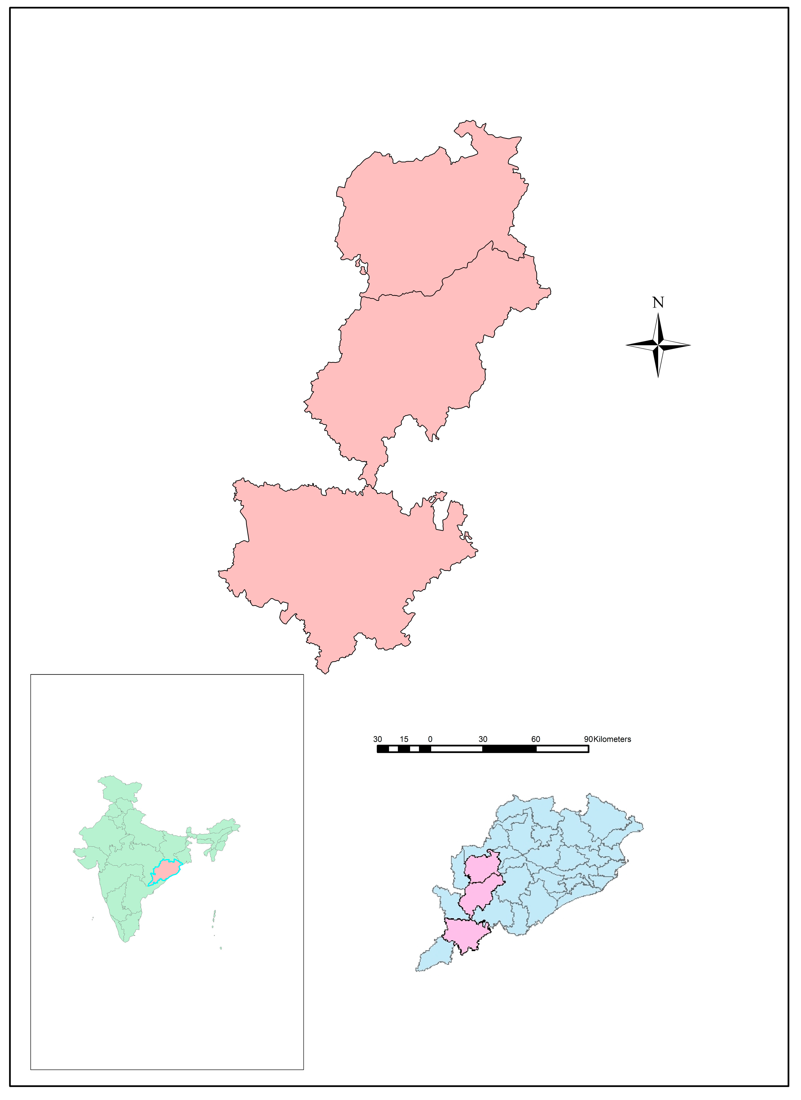
Figure 1. Location map of Kalahandi, Bolangir and, Koraput (KBK) districts.
Climate 07 00126 g001
Figure 2. Rice and maize yield anomaly and seasonal rainfall anomaly (1980–2017).
Climate 07 00126 g002
Figure 3. Relationship between rice and maize yield deficiency years, along with rainfall and temperature deviation years.
Climate 07 00126 g003
Figure 4. Correlation coefficients (r) values for rice and maize yield anomaly, along with rainfall anomaly.
Climate 07 00126 g004
Figure 5. Correlation coefficients (r) values for rice and maize yield, along with temperature anomaly.
Climate 07 00126 g005
Table 1. Years representing paddy and maize yield deficient years (>10%), along with rainfall and temperature deviation years.
Rainfall Deviation Years > 10%Temperature Deviation Years > 10%Rice Yield Deficient Years > 10%Maize Yield Deficient Years > 10%
1982−25.44198131.221982–3−33.111981–82−23.12
1983−37.46198510.121984–85−23.311983–84−21.32
1984−29.34198611.811987–88−43.611984–85−39.60
1987−18.55198912.891988–89−14.701988–89−17.80
1988−32.57199210.231996–97−57.401991–92−46.21
1990−10.23199511.902000–01−62.792000–01−24.68
1991−14.32199813.762002–03−75.672003–04−31.90
2000−55.32200324.682004–05−21.342006–7−19.60
2001−22.78200632.202008–09−11.882012–13−47.08
2002−40.07201229.802009–10−18.812014–15−66.59
2004−45.99201434.872010–11−26.522016–17−77.67
2005−24.84201541.982011–12−87.23
2009−42.65201638.652015–16−41.43
2010−90.07
Table 2. Multiple linear regression analysis for maize and rice yield.
Rice Yield
(Rainfall Anomaly)
Maize Yield
(Rainfall Anomaly)
Multiple R0.8560.738
R20.7320.544
Beta0.8560.738
Sig0.0180.044
Table 3. Monsoon Index (MI) with 5-year running mean of rice and maize.
Monsoon Index (MI)RiceMaize
YieldProductionYieldProduction
MI-JJA0.610.500.550.49
MI-JAS0.660.540.590.51
MI-JJAS0.600.550.560.43
Table 4. Linear regression analysis for maize and rice yield.
Rice Yield
(MI-JJA)
Rice Yield
(MI-JJAS)
Maize Yield
(MI-JJA)
Maize Yield
(MI-JJAS)
R 0.65 0.51 0.56 0.48
R20.42 0.26 0.31 0.23
Beta 0.65 0.51 0.56 0.48
Sig 0.013 0.023 0.034 0.04
Table 5. Correlation of ONI, NINO-3, and NINO-3.4 with 5-year running mean of rice and maize.
ONININO-3NINO-3.4
NDJDJFNDJDJFNDJDJF
RiceYield0.390.420.320.390.320.35
Production0.350.380.320.340.340.36
MaizeYield0.410.430.390.330.380.39
Production0.360.390.400.340.380.36