Feasibility of Predicting Vietnam’s Autumn Rainfall Regime Based on the Tree-Ring Record and Decadal Variability

 , , ,
, , ,
Abstract
:1. Introduction
2. Materials and Methods
3. Results
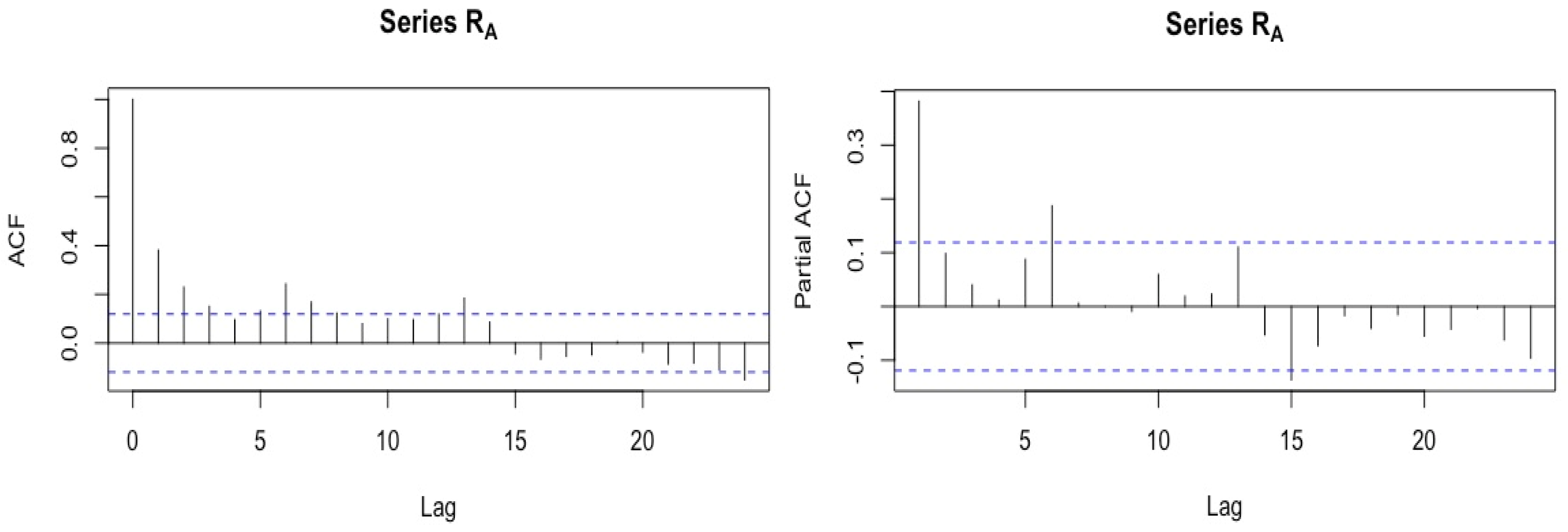
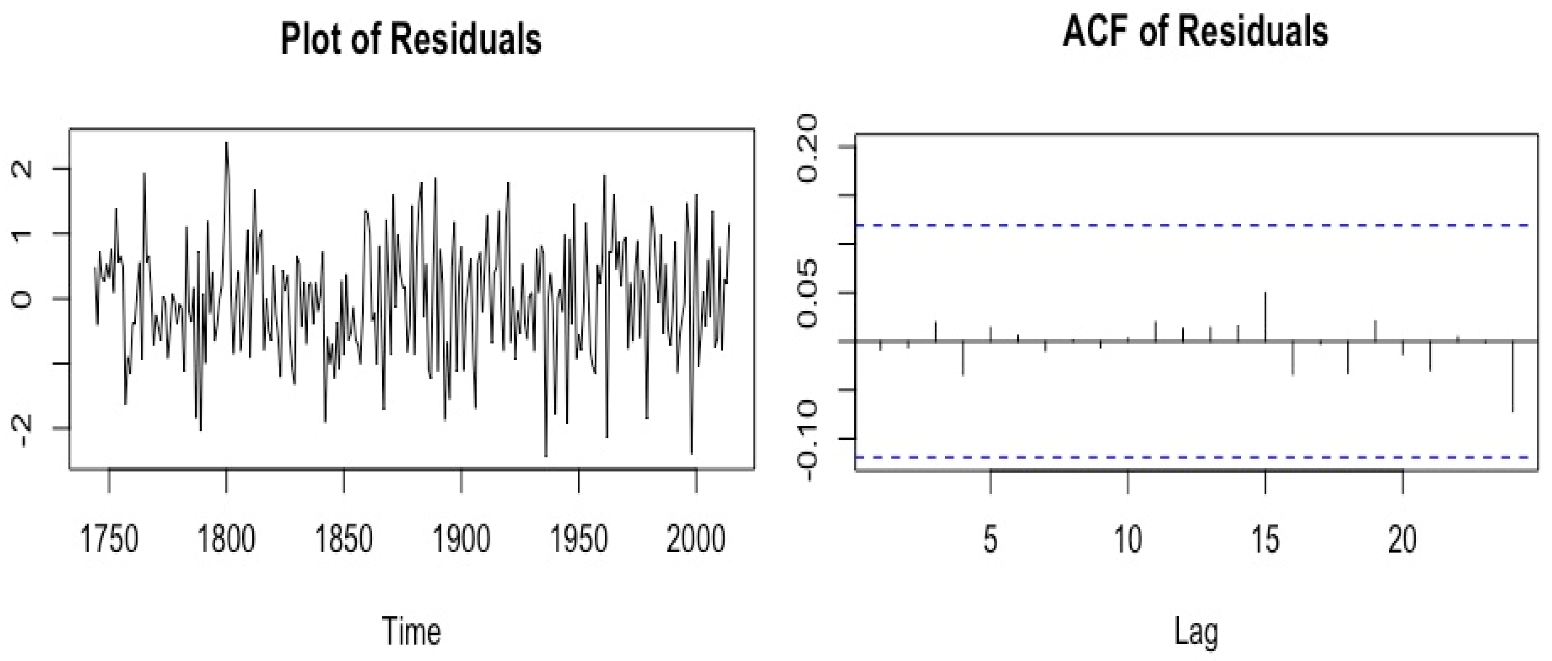
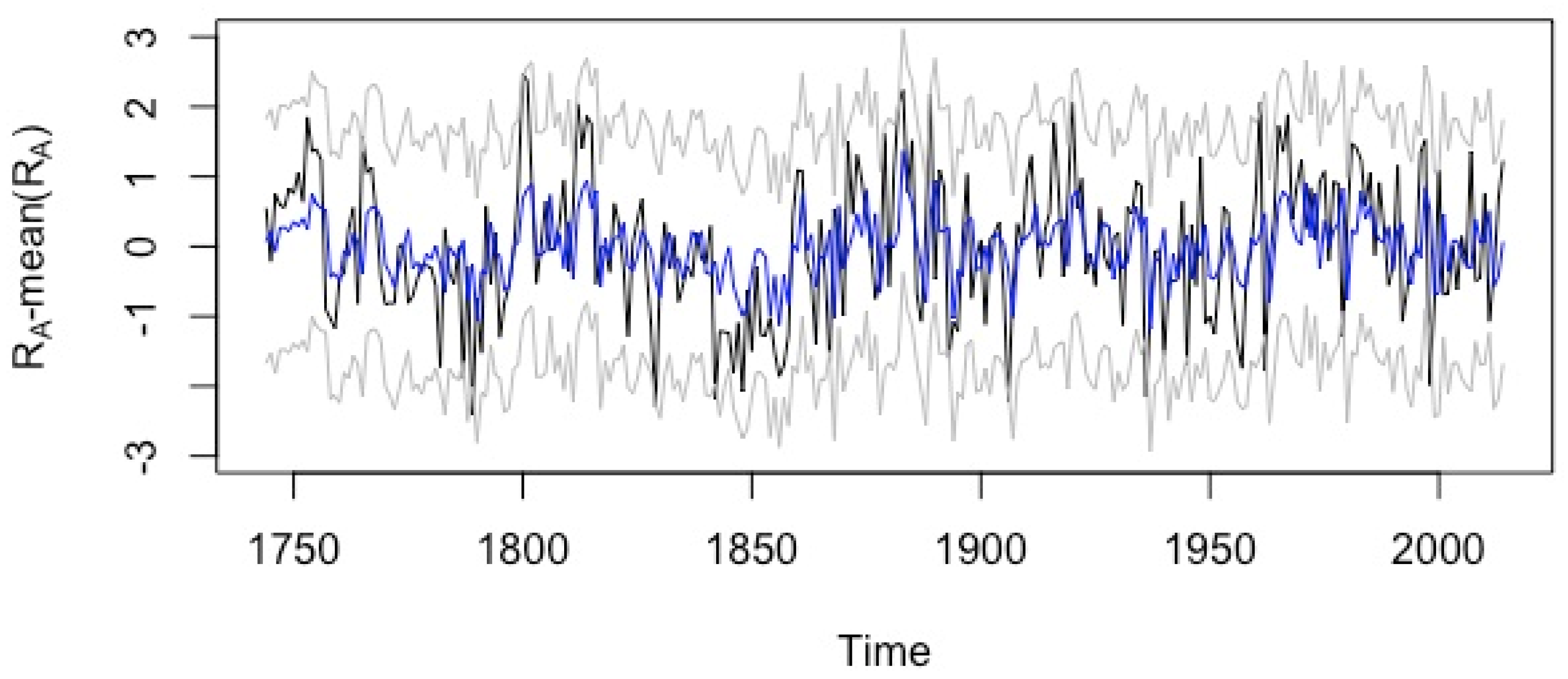
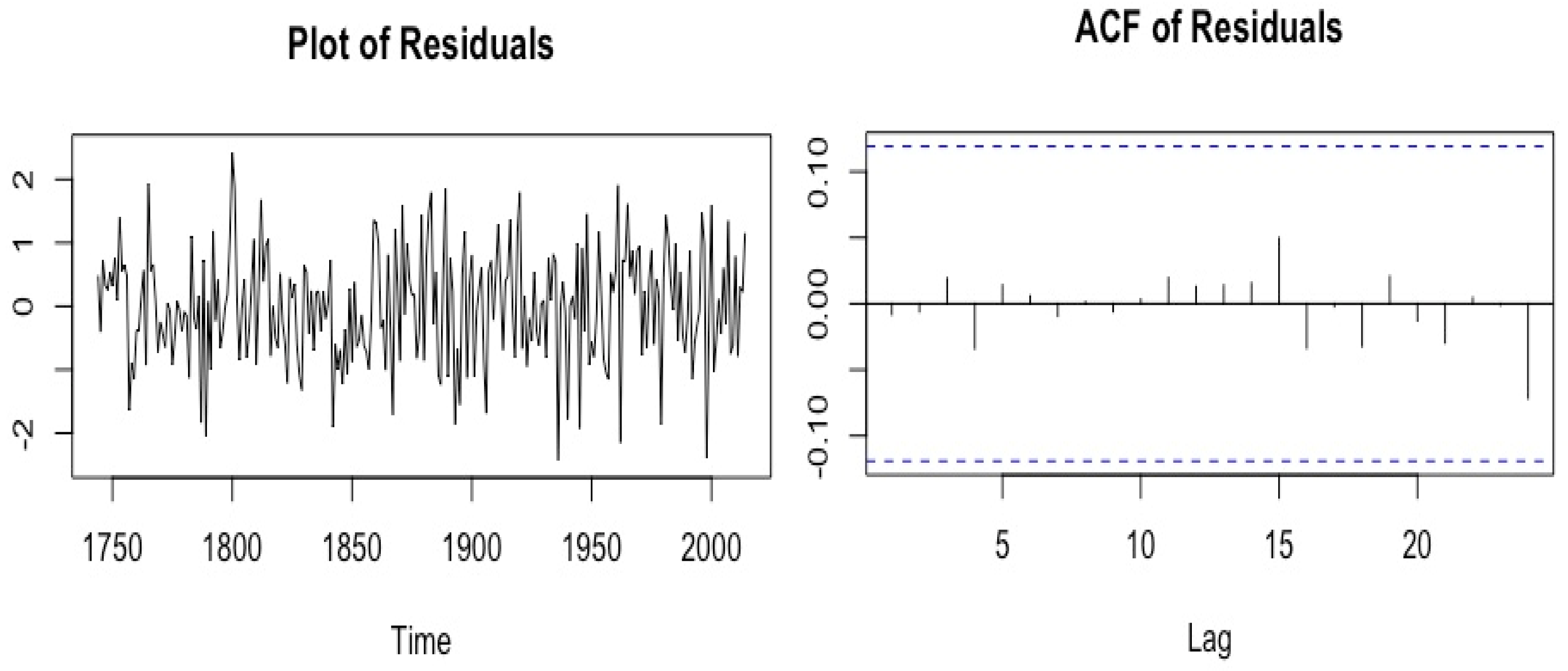
3.1. ARMA Model
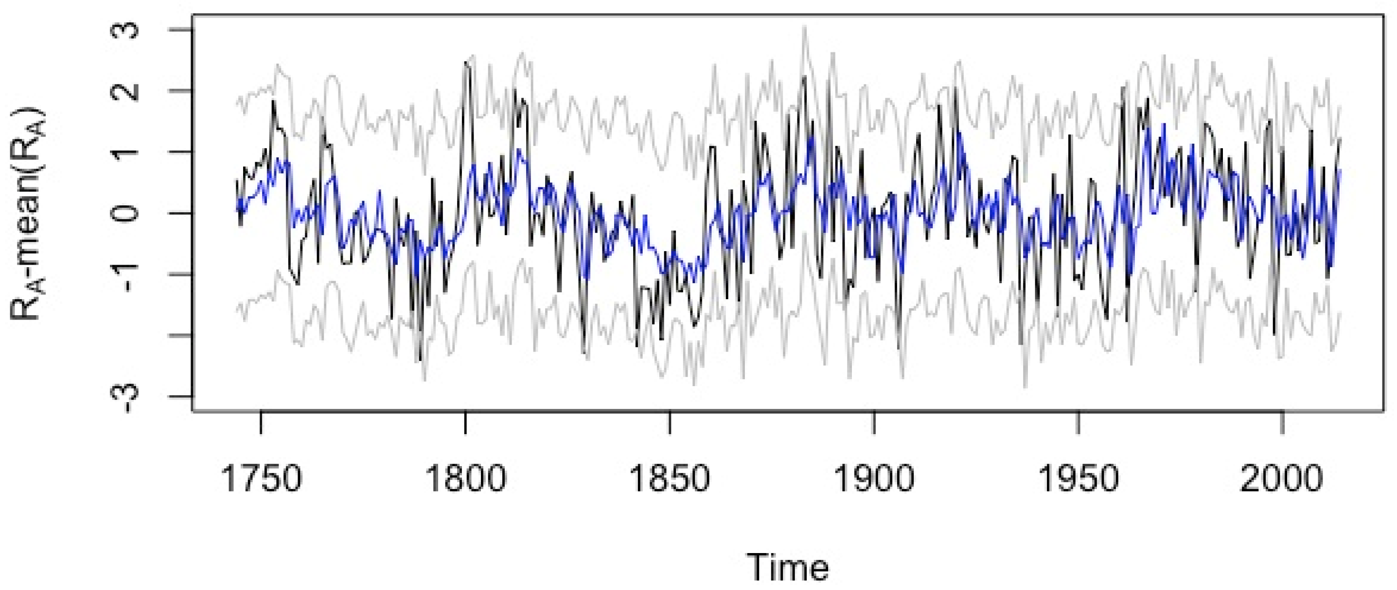
3.2. Long-Order Sparse AR (SpsAR) Model
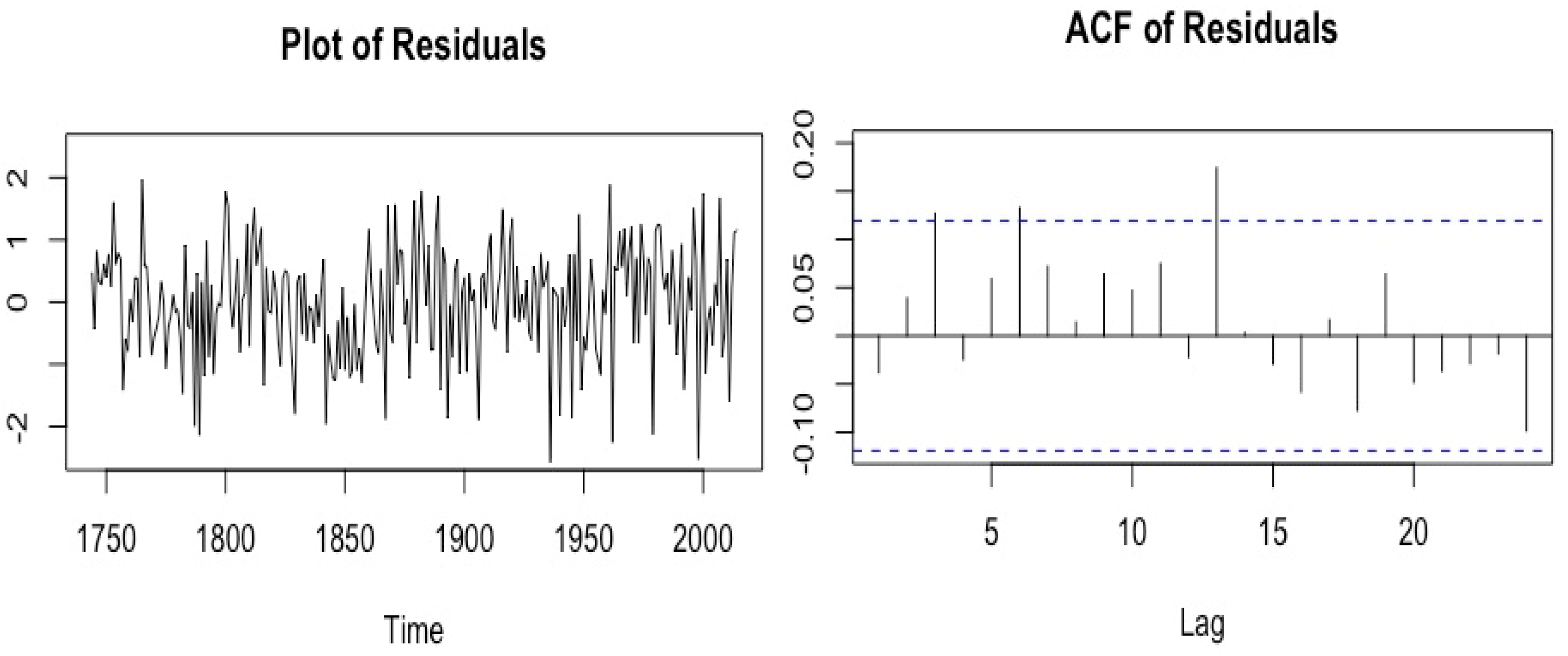
3.3. ARMAX Model
3.4. Sparse ARX Model
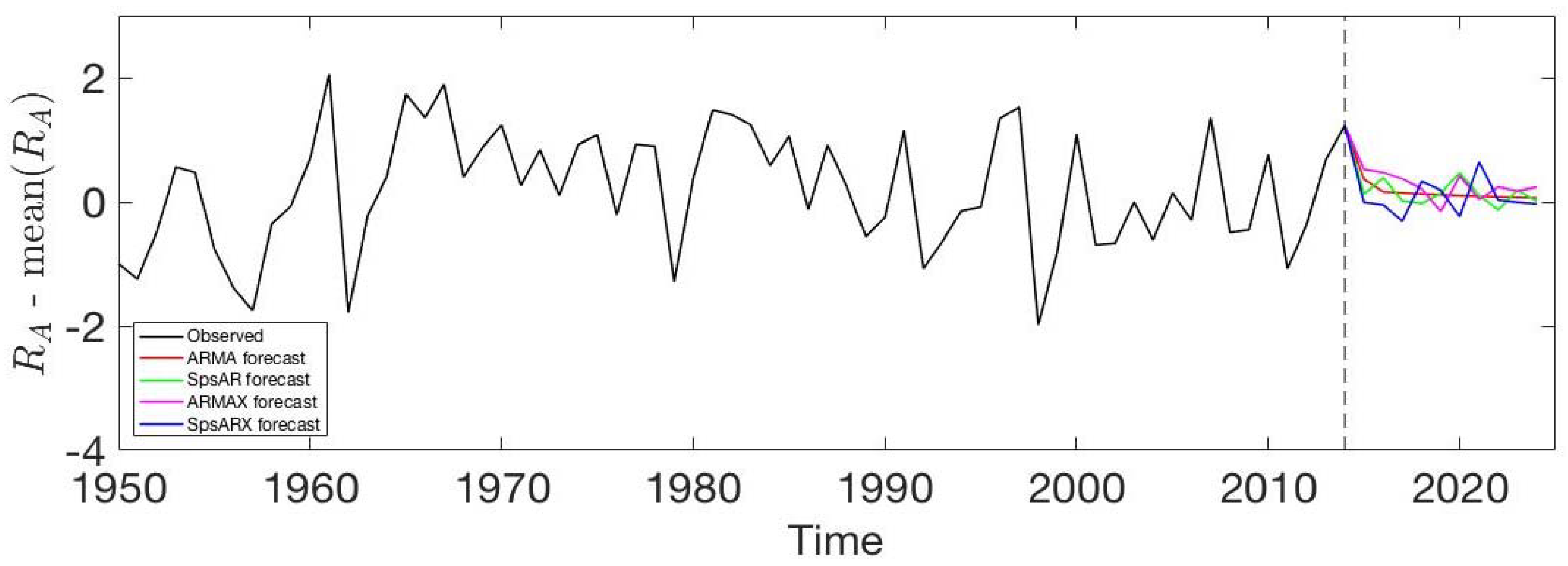
3.5. Forecasting Accuracy
4. Summary and Discussion
Author Contributions
Acknowledgments
Conflicts of Interest
References
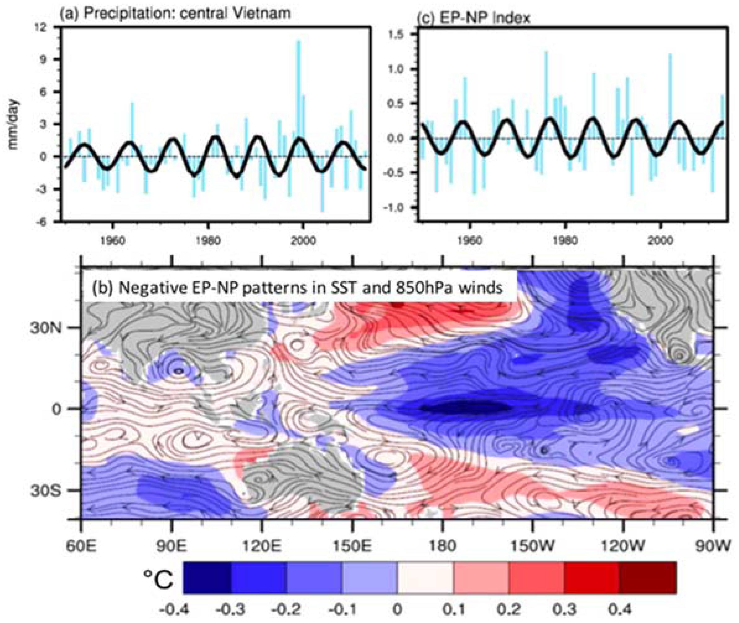
- Li, R.; Wang, S.Y.; Gillies, R.R.; Buckley, B.; Troung, L.H.; Cho, C. Decadal oscillation of autumn precipitation in Central Vietnam modulated by the East Pacific–North Pacific (EP–NP) teleconnection. Environ. Res. Lett. 2015, 10, 024008. [Google Scholar] [CrossRef]
- Nguyen, D.Q.; Renwick, J.; McGregor, J. Variations of surface temperature and rainfall in Vietnam from 1971 to 2010. Int. J. Climatol. 2014, 34, 249–264. [Google Scholar] [CrossRef]
- Wang, S.Y.S.; Promchote, P.; Truong, L.H.; Buckley, B.M.; Li, R.; Gillies, R.; Trung, N.T.Q.; Buan, B.; Minh, T.T. Changes in the autumn precipitation and tropical cyclone activity over Central Vietnam and its East Sea. Vietnam J. Earth Sci. 2015, 36, 489–496. [Google Scholar] [CrossRef]
- Yokoi, S.; Matsumoto, J. Collaborative effects of cold surge and tropical depression–type disturbance on heavy rainfall in central Vietnam. Mon. Weather. Rev. 2008, 136, 3275–3287. [Google Scholar] [CrossRef]
- Li, R.; Wang, S.Y.; Gillies, R.R.; Buckley, B.; Yoon, J.-H.; Cho, C. Regional trends in early-monsoon rainfall over Vietnam and CCSM4 attribution. Clim. Dyn. 2018, in press. [Google Scholar] [CrossRef]
- Buckley, B.M.; Stahle, D.K.; Luu, H.T. Central Vietnam climate over the past five centuries from cypress tree rings. Clim. Dyn. 2017, 48, 3707–3723. [Google Scholar] [CrossRef]
- Hansen, K.G.; Buckley, B.M.; Zottoli, B.; D’Arrigo, R.D.; Nam, L.C.; Truong, V.V.; Nguyen, D.T.; Nguyen, H.X. Discrete seasonal hydroclimate reconstructions over northern Vietnam for the past three and a half centuries. Clim. Chang. 2017, 145, 177–188. [Google Scholar] [CrossRef]
- Wilks, D. Statistical Methods in the Atmospheric Sciences, 3rd ed.; Academic Press: Oxford, UK, 2011; pp. 2–676. ISBN 9780123850225. [Google Scholar]


| 1-Step-Ahead | 2-Step-Ahead | 5-Step-Ahead | 10-Step-Ahead | ||||||
|---|---|---|---|---|---|---|---|---|---|
| RMSE | MSTE | RMSE | MSTE | RMSE | MSTE | RMSE | MSTE | SS | |
| ARMA (1,2) | 0.87883 | 0.91138 | 0.83087 | 0.95757 | 0.80310 | 0.98140 | 0.78911 | 0.99966 | 0.00265 |
| SpsAR (15) | 0.77737 | 0.87834 | 0.81207 | 0.91978 | 0.77672 | 0.94083 | 0.78770 | 0.96606 | 0.00620 |
| ARMAX (1,0,6) | 0.98435 | 0.88835 | 0.99321 | 0.95844 | 0.94871 | 0.97373 | 0.94790 | 0.97407 | −0.43912 |
| SpsARX (15,6) | 0.63692 | 0.86983 | 0.62585 | 0.90789 | 0.58614 | 0.93281 | 0.58306 | 0.96902 | 0.45550 |
| 1-Step-Ahead | 2-Step-Ahead | 5-Step-Ahead | 10-Step-Ahead | |||||
|---|---|---|---|---|---|---|---|---|
| RMSE | MSTE | RMSE | MSTE | RMSE | MSTE | RMSE | MSTE | |
| ARMA (1,2) | 0.94291 | 0.91012 | 0.97659 | 0.96582 | 0.97619 | 1.00022 | 0.98199 | 1.00556 |
| SpsAR (15) | 0.92504 | 0.87843 | 0.89998 | 0.91994 | 0.92794 | 0.94119 | 0.97126 | 0.96686 |
| ARMAX (1,0,6) | 0.98752 | 0.87852 | 1.03347 | 0.95508 | 1.02754 | 0.97091 | 1.03543 | 0.96946 |
| SpsARX (15,6) | 0.84880 | 0.87290 | 0.88449 | 0.91330 | 0.87881 | 0.94081 | 0.93695 | 0.97237 |
© 2018 by the authors. Licensee MDPI, Basel, Switzerland. This article is an open access article distributed under the terms and conditions of the Creative Commons Attribution (CC BY) license (http://creativecommons.org/licenses/by/4.0/).
Share and Cite
Sun, Y.; Wang, S.-Y.S.; Li, R.; Buckley, B.M.; Gillies, R.; Hansen, K.G. Feasibility of Predicting Vietnam’s Autumn Rainfall Regime Based on the Tree-Ring Record and Decadal Variability. Climate 2018, 6, 42. https://doi.org/10.3390/cli6020042
Sun Y, Wang S-YS, Li R, Buckley BM, Gillies R, Hansen KG. Feasibility of Predicting Vietnam’s Autumn Rainfall Regime Based on the Tree-Ring Record and Decadal Variability. Climate. 2018; 6(2):42. https://doi.org/10.3390/cli6020042
Chicago/Turabian StyleSun, Yan, S. -Y. Simon Wang, Rong Li, Brendan M. Buckley, Robert Gillies, and Kyle G. Hansen. 2018. "Feasibility of Predicting Vietnam’s Autumn Rainfall Regime Based on the Tree-Ring Record and Decadal Variability" Climate 6, no. 2: 42. https://doi.org/10.3390/cli6020042
APA StyleSun, Y., Wang, S.-Y. S., Li, R., Buckley, B. M., Gillies, R., & Hansen, K. G. (2018). Feasibility of Predicting Vietnam’s Autumn Rainfall Regime Based on the Tree-Ring Record and Decadal Variability. Climate, 6(2), 42. https://doi.org/10.3390/cli6020042