
Towards Systematic Prediction of Urban Heat Islands: Grounding Measurements, Assessing Modeling Techniques


Abstract
:
1. Introduction
2. Materials and Methods
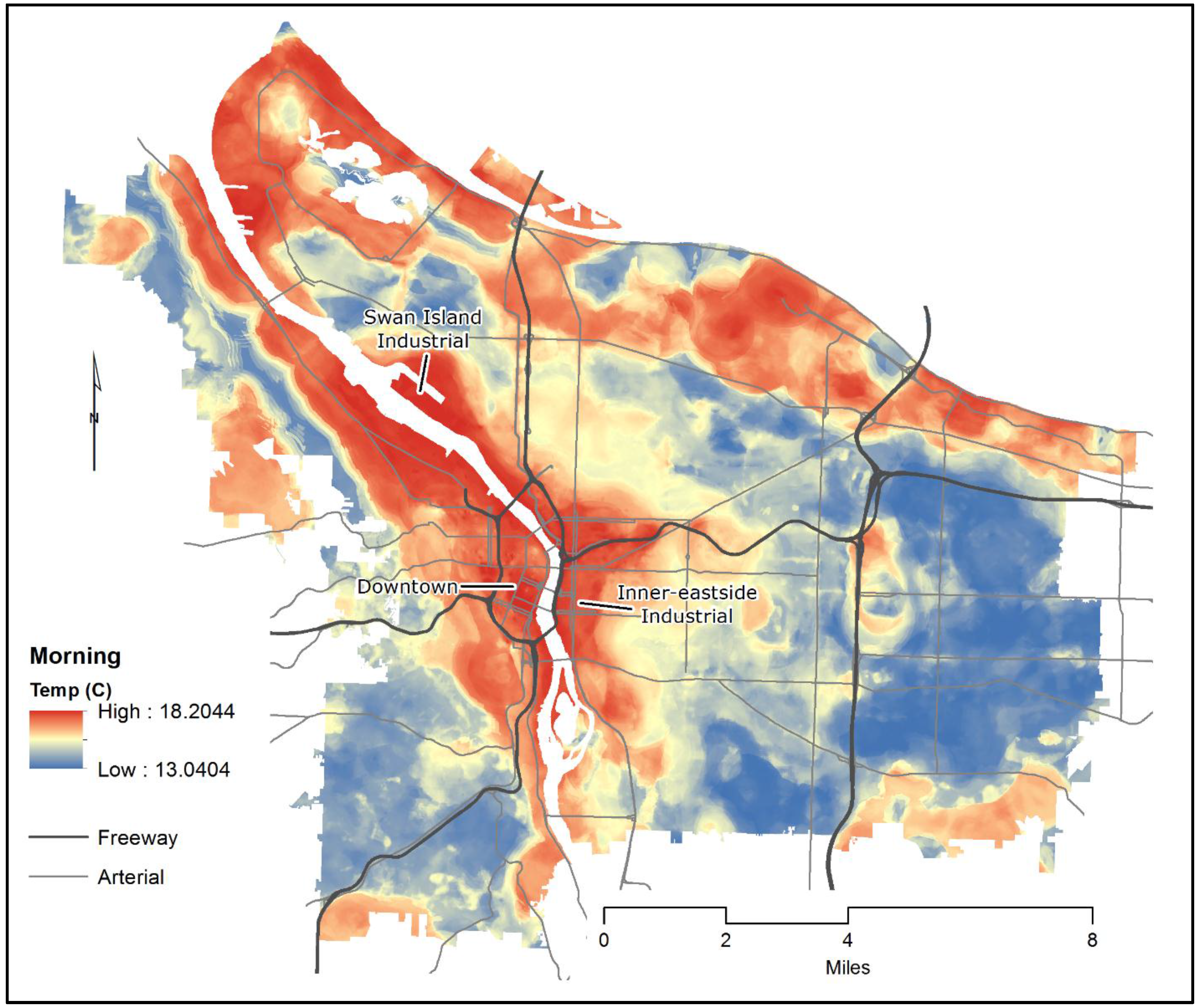
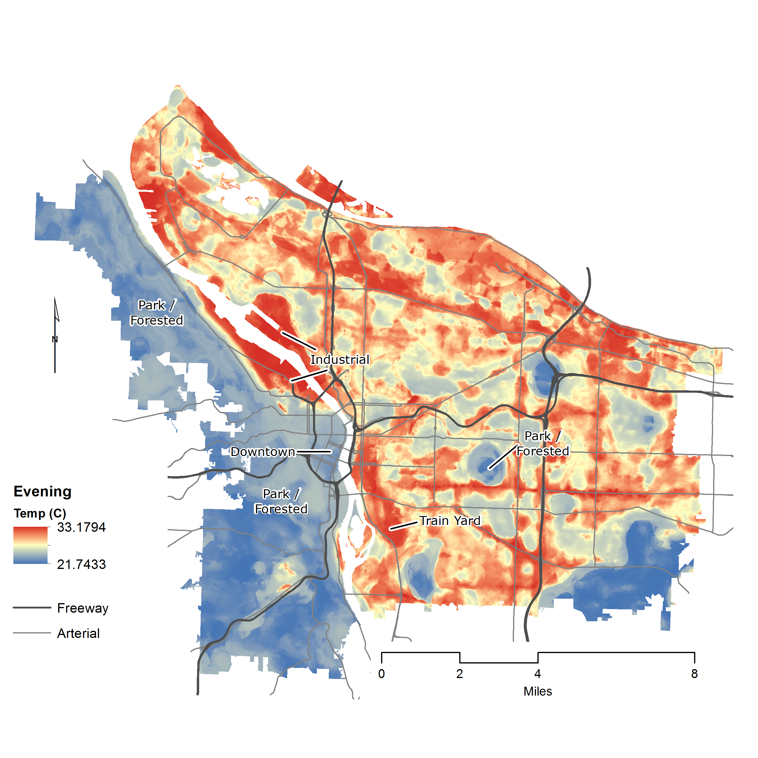
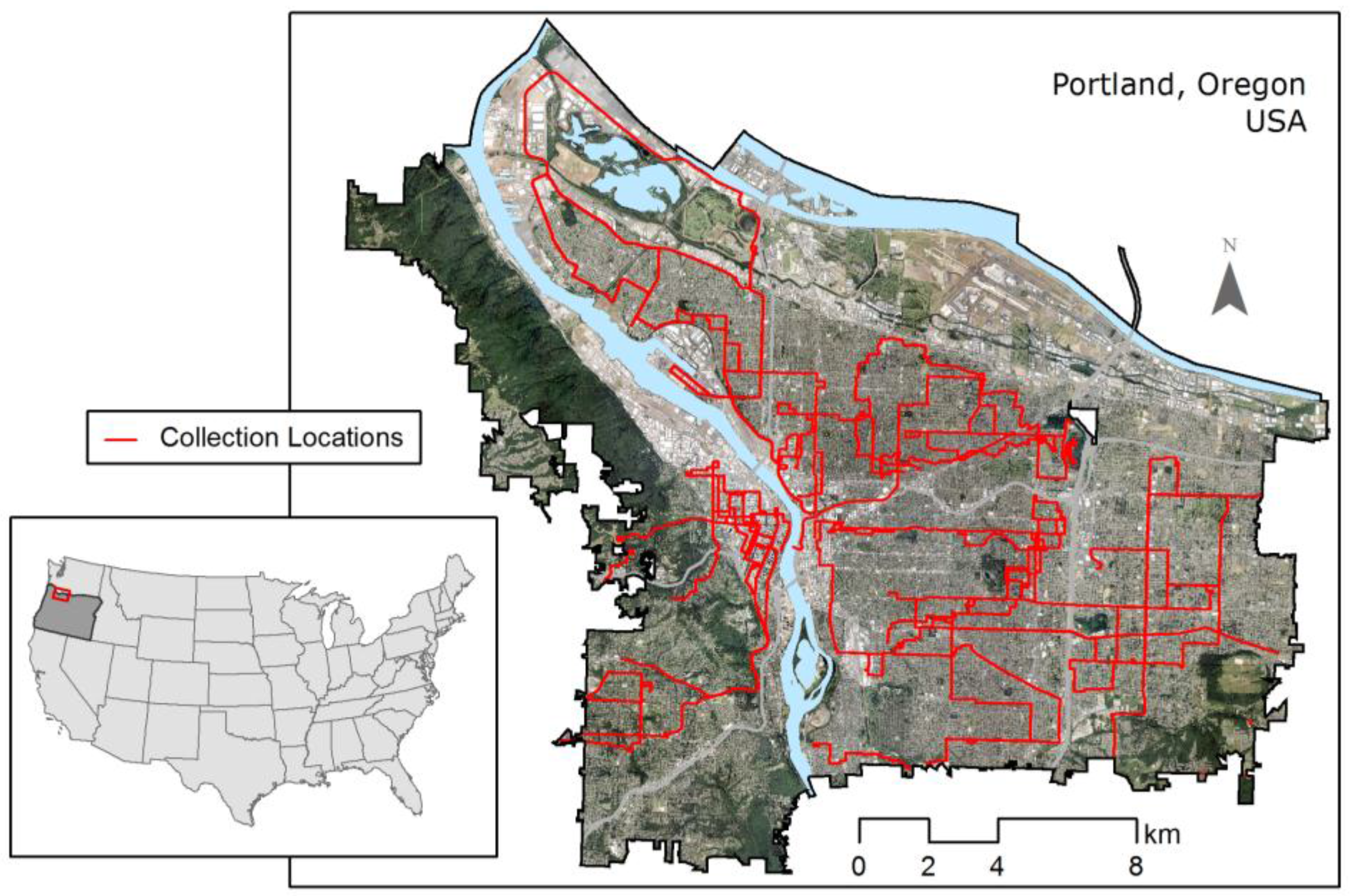
2.1. Study Area
2.2. Data
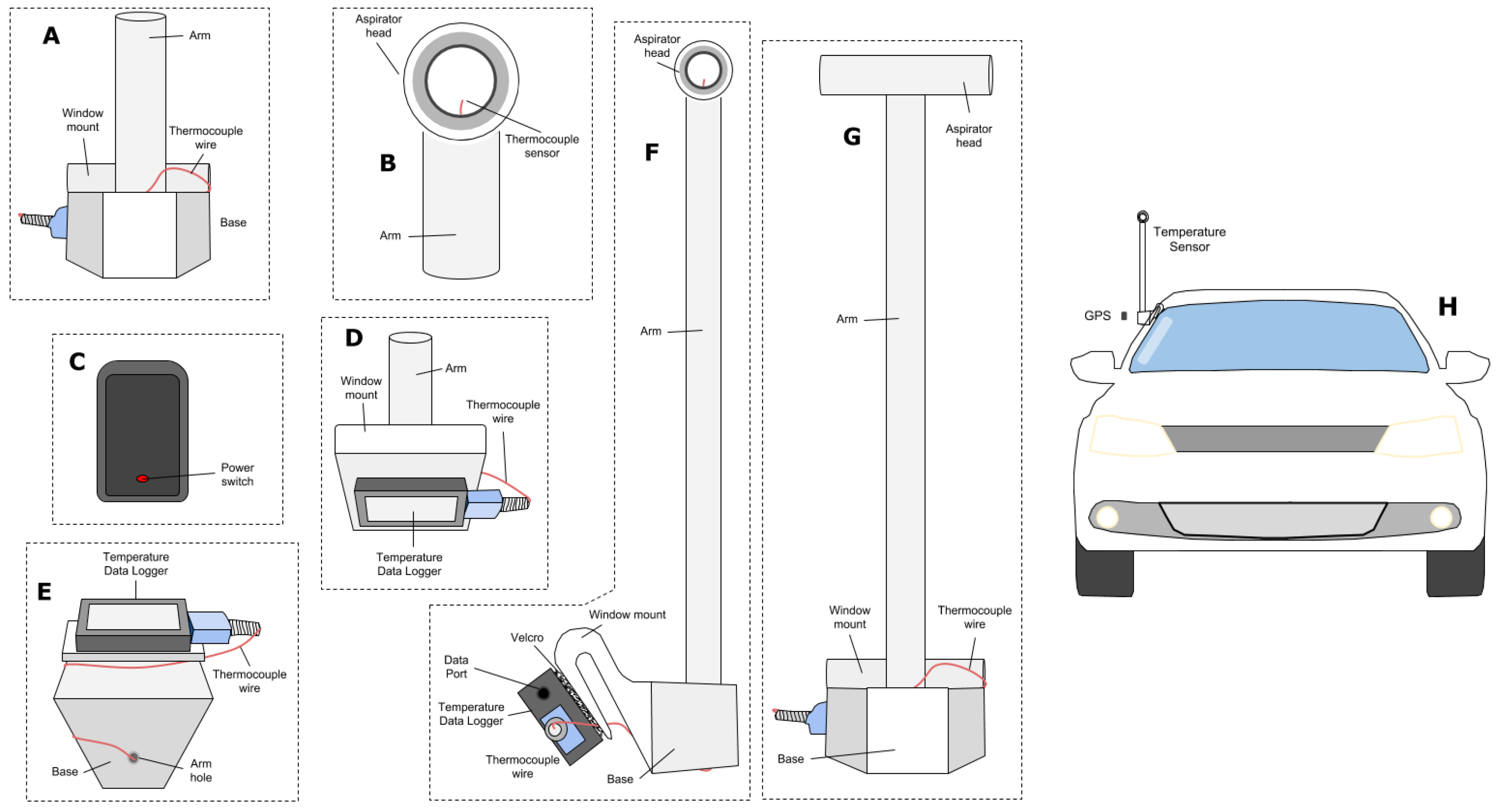
2.2.1. Temperature Data Collection and Compilation
2.2.2. LiDAR Data
2.2.3. Orthophotography Data
2.2.4. Building Data
2.2.5. Canopied and Non-Canopied Vegetation
2.2.6. Canopy Density Metric
2.2.7. Elevation
2.3. Modeling
2.3.1. Effective Distances
2.3.2. Model Validity
2.3.3. Multiple Linear Regression (MLR)
2.3.4. Classification and Regression Tree/Multiple Linear Regression Hybrid
2.3.5. Random Forest Analysis
3. Results
3.1. Multiple Linear Regression (MLR)
3.2. Classification and Regression Tree/Multiple Linear Regression Hybrid
3.3. Classification and Regression Tree/Multiple Linear Regression Hybrid
3.3.1. Random Forest: Morning Results
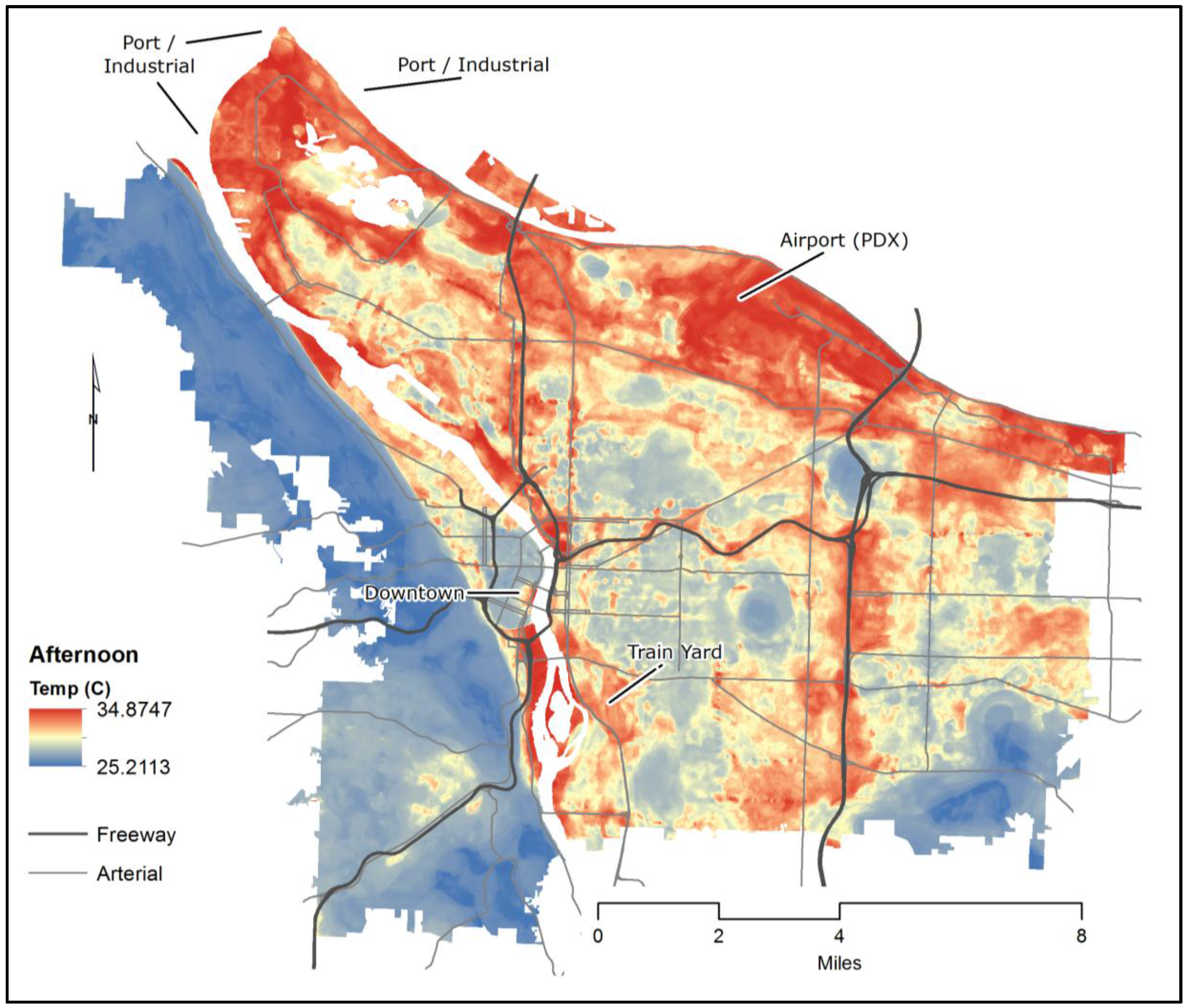
3.3.2. Random Forest: Afternoon Results
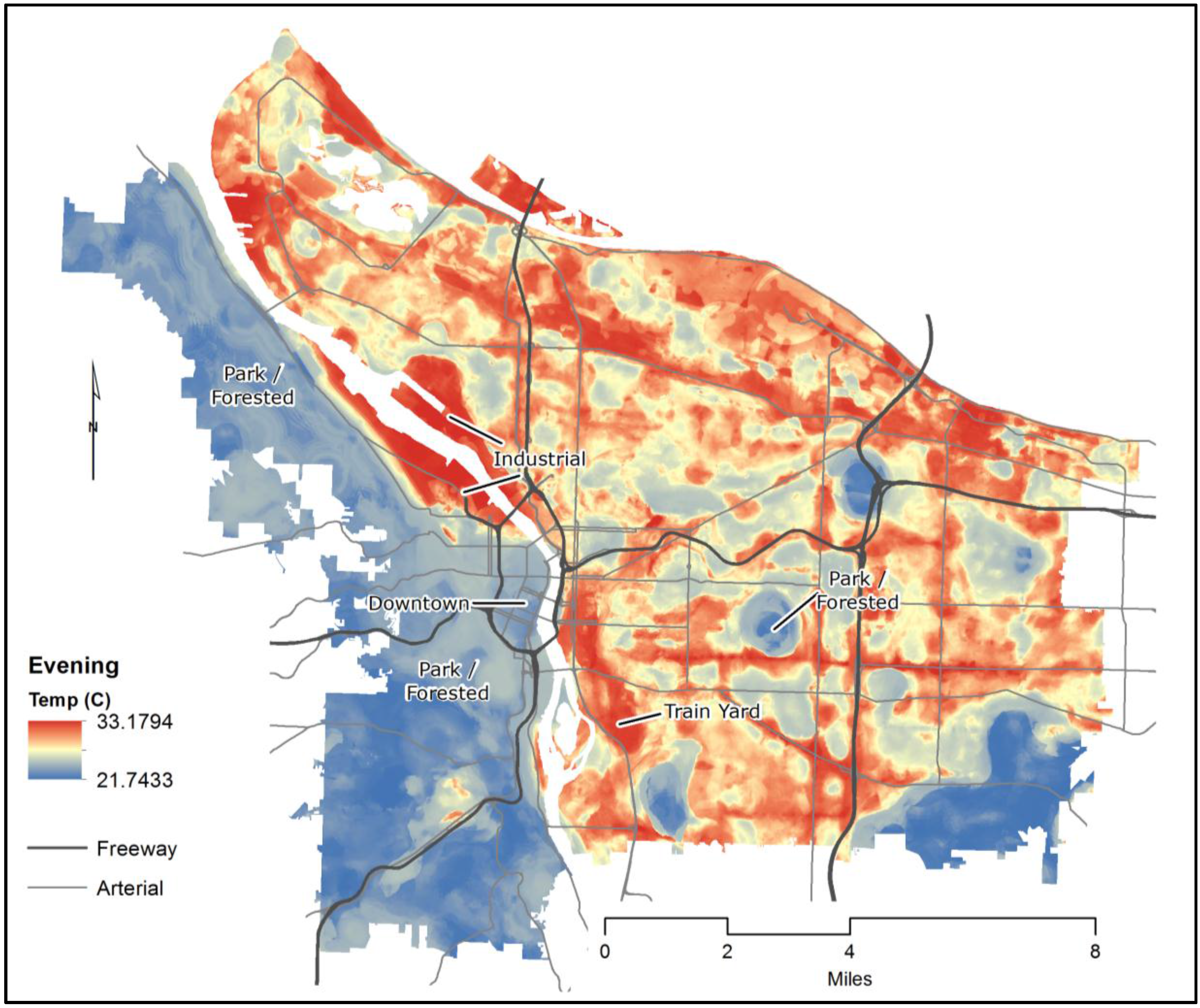
3.3.3. Random Forest: Evening Results
4. Discussion
5. Conclusions
Acknowledgments
Author Contributions
Conflicts of Interest
References
- Poumadère, M.; Mays, C.; Le Mer, S.; Blong, R. The 2003 Heat Wave in France: Dangerous Climate Change Here and Now. Risk Anal. 2005, 25, 1483–1494. [Google Scholar] [CrossRef] [PubMed]
- Borden, K.A.; Cutter, S.L. Spatial patterns of natural hazards mortality in the United States. Int. J. Health Geogr. 2008, 7, 64. [Google Scholar] [CrossRef] [PubMed]
- Henry, J.A.; Dicks, S.E. Association of urban temperatures with land use and surface materials. Landsc. Urban Plan. 1987, 14, 21–29. [Google Scholar] [CrossRef]
- Oke, T.R. The energetic basis of the urban heat island. Q. J. R. Meteorol. Soc. 1982, 108, 1–24. [Google Scholar] [CrossRef]
- United Nations World Urbanization Prospects: The 2014 Revision; Department of Economic and Social Affairs, Population Division: New York, NY, USA, 2015.
- Meehl, G.A.; Tebaldi, C. More Intense, More Frequent, and Longer Lasting Heat Waves in the 21st Century. Science 2004, 305, 994–997. [Google Scholar] [CrossRef] [PubMed]
- Howard, L. The Climate of London: Deduced from Meteorological Observations Made at Different Places in the Neighbourhood of the Metropolis; In Two Volumes; W. Phillips: London, UK, 1820. [Google Scholar]
- Voelkel, J.; Shandas, V.; Haggerty, B. Developing High-Resolution Descriptions of Urban Heat Islands: A Public Health Imperative. Prev. Chronic Dis. 2016. [Google Scholar] [CrossRef] [PubMed]
- Mees, H.L.P.; Driessen, P.P.J.; Runhaar, H.A.C. “Cool” governance of a “hot” climate issue: Public and private responsibilities for the protection of vulnerable citizens against extreme heat. Reg. Environ. Chang. 2015, 15, 1065–1079. [Google Scholar] [CrossRef]
- Weng, Q.; Lu, D.; Schubring, J. Estimation of land surface temperature–vegetation abundance relationship for urban heat island studies. Remote Sens. Environ. 2004, 89, 467–483. [Google Scholar] [CrossRef]
- Baldinelli, G.; Bonafoni, S. Analysis of Albedo Influence on Surface Urban Heat Island by Spaceborne Detection and Airborne Thermography. In New Trends in Image Analysis and Processing—ICIAP 2015 Workshops; Murino, V., Puppo, E., Sona, D., Cristani, M., Sansone, C., Eds.; Springer International Publishing: Genoa, Italy, 2015; pp. 95–102. [Google Scholar]
- Cao, X.; Onishi, A.; Chen, J.; Imura, H. Quantifying the cool island intensity of urban parks using ASTER and IKONOS data. Landsc. Urban Plan. 2010, 96, 224–231. [Google Scholar] [CrossRef]
- Mallick, J.; Rahman, A.; Singh, C.K. Modeling urban heat islands in heterogeneous land surface and its correlation with impervious surface area by using night-time ASTER satellite data in highly urbanizing city, Delhi-India. Adv. Space Res. 2013, 52, 639–655. [Google Scholar] [CrossRef]
- Lee, L.; Chen, L.; Wang, X.; Zhao, J. Use of Landsat TM/ETM+ data to analyze urban heat island and its relationship with land use/cover change. In Proceedings of the 2011 International Conference on Remote Sensing, Environment and Transportation Engineering (RSETE), Nanjing, China, 24–26 June 2011; pp. 922–927. [Google Scholar]
- Grover, A.; Singh, R.B. Analysis of Urban Heat Island (UHI) in Relation to Normalized Difference Vegetation Index (NDVI): A Comparative Study of Delhi and Mumbai. Environments 2015, 2, 125–138. [Google Scholar] [CrossRef]
- Hamstead, Z.A.; Kremer, P.; Larondelle, N.; McPhearson, T.; Haase, D. Classification of the heterogeneous structure of urban landscapes (STURLA) as an indicator of landscape function applied to surface temperature in New York City. Ecol. Indic. 2016, 70, 574–585. [Google Scholar] [CrossRef]
- Sobrino, J.A.; Oltra-Carrió, R.; Sòria, G.; Bianchi, R.; Paganini, M. Impact of spatial resolution and satellite overpass time on evaluation of the surface urban heat island effects. Remote Sens. Environ. 2012, 117, 50–56. [Google Scholar] [CrossRef]
- Chandler, T.J. Temperature and Humidity Traverses across London. Weather 1962, 17, 235–242. [Google Scholar] [CrossRef]
- Song, B.; Park, K.; Song, B.; Park, K. Validation of ASTER Surface Temperature Data with In Situ Measurements to Evaluate Heat Islands in Complex Urban Areas, Validation of ASTER Surface Temperature Data with In Situ Measurements to Evaluate Heat Islands in Complex Urban Areas. Adv. Meteorol. 2014, 2014, e620410. [Google Scholar] [CrossRef]
- Saaroni, H.; Ben-Dor, E.; Bitan, A.; Potchter, O. Spatial distribution and microscale characteristics of the urban heat island in Tel-Aviv, Israel. Landsc. Urban Plan. 2000, 48, 1–18. [Google Scholar] [CrossRef]
- Hart, M.A.; Sailor, D.J. Quantifying the influence of land-use and surface characteristics on spatial variability in the urban heat island. Theor. Appl. Climatol. 2008, 95, 397–406. [Google Scholar] [CrossRef]
- Yokobori, T.; Ohta, S. Effect of land cover on air temperatures involved in the development of an intra-urban heat island. Clim. Res. 2009, 39, 61–73. [Google Scholar] [CrossRef]
- Kotharkar, R.; Surawar, M. Land Use, Land Cover, and Population Density Impact on the Formation of Canopy Urban Heat Islands through Traverse Survey in the Nagpur Urban Area, India. J. Urban Plan. Dev. 2016, 142, 4015003. [Google Scholar] [CrossRef]
- Makido, Y.; Shandas, V.; Ferwati, S.; Sailor, D. Daytime Variation of Urban Heat Islands: The Case Study of Doha, Qatar. Climate 2016, 4, 32. [Google Scholar] [CrossRef]
- Metro Data Resource Center Regional Land Information System (RLIS); Oregon Metro: Portland, OR, USA, 2014.
- NOAA Daily Temperatures—Extremes and Normals. Available online: http://www.wrh.noaa.gov/pqr/pdxclimate/pg6.pdf (accessed on 28 May 2016).
- Van Hove, L.W.A.; Jacobs, C.M.J.; Heusinkveld, B.G.; Elbers, J.A.; Van Driel, B.L.; Holtslag, A.A.M. Temporal and spatial variability of urban heat island and thermal comfort within the Rotterdam agglomeration. Build. Environ. 2015, 83, 91–103. [Google Scholar] [CrossRef]
- Simpson, J.R.; McPherson, E.G. Simulation of tree shade impacts on residential energy use for space conditioning in Sacramento. Atmos. Environ. 1998, 32, 69–74. [Google Scholar] [CrossRef]
- Bolund, P.; Hunhammar, S. Ecosystem services in urban areas. Ecol. Econ. 1999, 29, 293–301. [Google Scholar] [CrossRef]
- Chow, W.T.L.; Roth, M. Temporal dynamics of the urban heat island of Singapore. Int. J. Climatol. 2006, 26, 2243–2260. [Google Scholar] [CrossRef]
- Takebayashi, H.; Moriyama, M. Study on the urban heat island mitigation effect achieved by converting to grass-covered parking. Sol. Energy 2009, 83, 1211–1223. [Google Scholar] [CrossRef]
- Rouse, J.W., Jr.; Haas, R.H.; Schell, J.A.; Deering, D.W. Monitoring Vegetation Systems in the Great Plains with Erts. In Proceedings of the 3rd Earth Resources Technology Satellite-1 Symposium, Washington, DC, USA, 10–14 December 1973. [Google Scholar]
- Moges, S.M.; Raun, W.R.; Mullen, R.W.; Freeman, K.W.; Johnson, G.V.; Solie, J.B. Evaluation of Green, Red, and Near Infrared Bands for Predicting Winter Wheat Biomass, Nitrogen Uptake, and Final Grain Yield. J. Plant Nutr. 2005, 27, 1431–1441. [Google Scholar] [CrossRef]
- Malthus, T.; Younger, C.J. Remotely sensing stress in street trees using high spatial resolution imagery. In Proceedings of the Second International Geospatial Information in Agriculture and Forestry Conference, Lake Buena Vista, FL, USA, 10–12 January 2000; ERIM International: Ann Arbor, MI, USA; Volume 2, pp. 326–333. [Google Scholar]
- Evans, J.S.; Hudak, A.T.; Faux, R.; Smith, A.M.S. Discrete Return LiDAR in Natural Resources: Recommendations for Project Planning, Data Processing, and Deliverables. Remote Sens. 2009, 1, 776–794. [Google Scholar] [CrossRef]
- Montgomery, D.C.; Peck, E.A.; Vining, G.G. Introduction to Linear Regression Analysis; John Wiley & Sons: Hoboken, NJ, USA, 2015. [Google Scholar]
- Zuur, A.F.; Ieno, E.N.; Elphick, C.S. A protocol for data exploration to avoid common statistical problems. Methods Ecol. Evol. 2010, 1, 3–14. [Google Scholar] [CrossRef]
- R Development Core Team. R: A Language and Environment for Statistical Computing; R Foundation for Statistical Computing: Vienna, Austria, 2016. [Google Scholar]
- Hijmans, R.J. Raster: Geographic Data Analysis and Modeling; The Comprehensive R Network: Vienna, Austria, 2015. [Google Scholar]
- Hansen, M.C.; DeFries, R.S.; Townshend, J.R.G.; Sohlberg, R.; Dimiceli, C.; Carroll, M. Towards an operational MODIS continuous field of percent tree cover algorithm: Examples using AVHRR and MODIS data. Remote Sens. Environ. 2002, 83, 303–319. [Google Scholar] [CrossRef]
- Yuan, F.; Wu, C.; Bauer, M.E. Comparison of Spectral Analysis Techniques for Impervious Surface Estimation Using Landsat Imagery. Photogramm. Eng. Remote Sens. 2008, 74, 1045–1055. [Google Scholar] [CrossRef]
- Breiman, L.; Friedman, J.; Stone, C.J.; Olshen, R.A. Classification and Regression Trees, 1st ed.; Chapman and Hall/CRC: New York, NY, USA, 1984. [Google Scholar]
- Hastie, T.; Tibshirani, R.; Friedman, J.H. The elements of statistical learning: Data mining, inference, and prediction. In Springer Series in Statistics, 2nd ed.; Springer: New York, NY, USA, 2009. [Google Scholar]
- Therneau, T.; Atkinson, B.; Ripley, B. rpart: Recursive Partitioning and Regression Trees; The Comprehensive R Network: Vienna, Austria, 2015. [Google Scholar]
- Liaw, A.; Wiener, M. Classification and Regression by randomForest. R News 2002, 2, 18–22. [Google Scholar]
- Lin, B.-S.; Lin, Y.-J. Cooling Effect of Shade Trees with Different Characteristics in a Subtropical Urban Park. HortScience 2010, 45, 83–86. [Google Scholar]
- Armson, D.; Stringer, P.; Ennos, A.R. The Effect of Tree Shade and Grass on Surface and Globe Temperatures in an Urban Area. Urban For. Urban Green. 2012, 11, 245–255. [Google Scholar] [CrossRef]
- Ellison, D.; Morris, C.E.; Locatelli, B.; Sheil, D.; Cohen, J.; Murdiyarso, D.; Gutierrez, V.; van Noordwijk, M.; Creed, I.F.; Pokorny, J.; et al. Trees, Forests and Water: Cool Insights for a Hot World. Glob. Environ. Chang. 2017, 43, 51–61. [Google Scholar] [CrossRef]
- Shashua-Bar, L.; Hoffman, M.E. Vegetation as a Climatic Component in the Design of an Urban Street: An Empirical Model for Predicting the Cooling Effect of Urban Green Areas with Trees. Energy Build. 2000, 31, 221–235. [Google Scholar] [CrossRef]
- Giridharan, R.; Ganesan, S.; Lau, S.S.Y. Daytime Urban Heat Island Effect in High-Rise and High-Density Residential Developments in Hong Kong. Energy Build. 2004, 36, 525–534. [Google Scholar] [CrossRef]
- Perini, K.; Magliocco, A. Effects of Vegetation, Urban Density, Building Height, and Atmospheric Conditions on Local Temperatures and Thermal Comfort. Urban For. Urban Green. 2014, 13, 495–506. [Google Scholar] [CrossRef]
- Gaffin, S.R.; Rosenzweig, C.; Khanbilvardi, R.; Parshall, L.; Mahani, S.; Glickman, H.; Goldberg, R.; Blake, R.; Slosberg, R.B.; Hillel, D. Variations in New York City’s Urban Heat Island Strength over Time and Space. Theor. Appl. Climatol. 2008, 94, 1–11. [Google Scholar] [CrossRef]
- Jian, H.; Li, Y.; Sandberg, M.; Buccolieri, R.; Sabatino, S.D. The Influence of Building Height Variability on Pollutant Dispersion and Pedestrian Ventilation in Idealized High-Rise Urban Areas. Build Environ. 2012, 56, 346–360. [Google Scholar] [CrossRef]
- Nassar, A.K.; Blackburn, G.A.; Whyatt, D. Developing the desert: The pace and process of urban growth in Dubai. Comput. Environ. Urban Syst. 2014, 45, 50–62. [Google Scholar] [CrossRef]
- Taha, H. Modifying a Mesoscale Meteorological Model to Better Incorporate Urban Heat Storage: A Bulk-Parameterization Approach. J. Appl. Meteorol. 1999, 38, 466–473. [Google Scholar] [CrossRef]
- Loikith, P.C.; Waliser, D.E.; Lee, H.; Neelin, J.D.; Lintner, B.R.; McGinnis, S.A.; Mearns, L.O.; Kim, J. Evaluation of Large-Scale Meteorological Patterns Associated with Temperature Extremes in the NARCCAP Regional Climate Model Simulations. Clim. Dyn. 2015, 45, 3257–3274. [Google Scholar] [CrossRef]
- Semenza, J.C.; Rubin, C.H.; Falter, K.H.; Selanikio, J.D.; Flanders, W.D.; Howe, H.L.; Wilhelm, J.L. Heat-Related Deaths during the July 1995 Heat Wave in Chicago. N. Engl. J. Med. 1996, 335, 84–90. [Google Scholar] [CrossRef] [PubMed]
- Bouchama, A.; Knochel, J.P. Heat Stroke. N. Engl. J. Med. 2002, 346, 1978–1988. [Google Scholar] [CrossRef] [PubMed]
- Turner, B.L.; Kasperson, R.E.; Matson, P.A.; McCarthy, J.J.; Corell, R.W.; Christensen, L.; Eckley, N.; Kasperson, J.X.; Luers, A.; Martello, M.L.; et al. A framework for vulnerability analysis in sustainability science. Proc. Natl. Acad. Sci. USA 2003, 100, 8074–8079. [Google Scholar] [CrossRef] [PubMed]


| Time | Rank | Model | r2 | RMSE |
|---|---|---|---|---|
| 6 a.m. | 3 | MLR | 0.5912 | 0.6575 |
| 2 | CART/MLR | 0.8595 | 0.3758 | |
| 1 | Random Forest | 0.9793 | 0.1479 | |
| 3 p.m. | 3 | MLR | 0.4554 | 0.8406 |
| 2 | CART/MLR | 0.5681 | 0.7633 | |
| 1 | Random Forest | 0.8199 | 0.4798 | |
| 7 p.m. | 3 | MLR | 0.4290 | 0.9011 |
| 2 | CART/MLR | 0.6638 | 0.7086 | |
| 1 | Random Forest | 0.9715 | 0.2078 |
| Time | r2 | RMSE (°C) | Variables | Beta |
|---|---|---|---|---|
| 6 a.m. | 0.5912 | 0.6575 | Vegetation cover within 700 m | −0.6664 |
| Canopy cover within 450 m | −0.3925 | |||
| Sum of CDM within 900 m | −0.2710 | |||
| 3 p.m. | 0.4554 | 0.8406 | Sum of CDM within 1000 m | −0.5483 |
| Building volume within 800 m | −0.5128 | |||
| Mean building height within 350 m | −0.3541 | |||
| Sum of CDM within 50 m | −0.1652 | |||
| 7 p.m. | 0.4290 | 0.9011 | Building volume within 900 m | −0.5446 |
| Sum of CDM within 600 m | −0.4589 | |||
| Vegetation cover within 400 m | −0.2392 | |||
| Canopy cover within 150 m | −0.1673 |
| Model | Variable Rank | Variable | %IncMSE |
|---|---|---|---|
| 6 a.m. | 1 | Vegetation cover within 50 m | 42.48 |
| 2 | Vegetation cover within 800 m | 38.72 | |
| 3 | Building volume within 900 m | 33.90 | |
| 4 | Sum of CDM within 1000 m | 32.98 | |
| 5 | Mean building height 100 m | 32.69 | |
| 3 p.m. | 1 | Standard deviation of building height within 1000 m | 40.83 |
| 2 | Standard deviation of building height within 300 m | 39.12 | |
| 3 | Sum of CDM within 50 m | 38.94 | |
| 4 | Standard deviation of building height within 150 m | 38.66 | |
| 5 | Standard deviation of building height within 200 m | 38.54 | |
| 7 p.m. | 1 | Standard deviation of building height within 1000 m | 39.95 |
| 2 | Vegetation cover within 100 m | 32.53 | |
| 3 | Building volume within 1000 m | 30.93 | |
| 4 | Canopy cover within 800 m | 30.91 | |
| 5 | Building volume within 900 m | 30.58 |
© 2017 by the authors. Licensee MDPI, Basel, Switzerland. This article is an open access article distributed under the terms and conditions of the Creative Commons Attribution (CC BY) license (http://creativecommons.org/licenses/by/4.0/).
Share and Cite
Voelkel, J.; Shandas, V. Towards Systematic Prediction of Urban Heat Islands: Grounding Measurements, Assessing Modeling Techniques. Climate 2017, 5, 41. https://doi.org/10.3390/cli5020041
Voelkel J, Shandas V. Towards Systematic Prediction of Urban Heat Islands: Grounding Measurements, Assessing Modeling Techniques. Climate. 2017; 5(2):41. https://doi.org/10.3390/cli5020041
Chicago/Turabian StyleVoelkel, Jackson, and Vivek Shandas. 2017. "Towards Systematic Prediction of Urban Heat Islands: Grounding Measurements, Assessing Modeling Techniques" Climate 5, no. 2: 41. https://doi.org/10.3390/cli5020041
APA StyleVoelkel, J., & Shandas, V. (2017). Towards Systematic Prediction of Urban Heat Islands: Grounding Measurements, Assessing Modeling Techniques. Climate, 5(2), 41. https://doi.org/10.3390/cli5020041