Article

Climate Change in Afghanistan Deduced from Reanalysis and Coordinated Regional Climate Downscaling Experiment (CORDEX)—South Asia Simulations

1
United Nations Environment Programme (UNEP) Post-conflict and Disaster Management Branch (PCDMB), UNOCA Compound, Kabul, Afghanistan
2
Potsdam Institute for Climate Impact Research (PIK), Am Telegraphenberg, 14473 Potsdam, Germany
3
Faculty of Environmental Science, University of Kabul, Jamal Mena Karte-e-Sakhi, Kabul, Afghanistan, [email protected]
4
Institute of Geography and Geology, University of Würzburg, Am Hubland, 97074 Würzburg, Germany
5
Institute of Ecology, Technical University of Berlin, Ernst-Reuter-Platz 1, 10587 Berlin, Germany
*
Author to whom correspondence should be addressed.
Climate 2017, 5(2), 38; https://doi.org/10.3390/cli5020038
Submission received: 20 March 2017 / Revised: 28 April 2017 / Accepted: 16 May 2017 / Published: 23 May 2017

Abstract

:
Past and the projected future climate change in Afghanistan has been analyzed systematically and differentiated with respect to its different climate regions to gain some first quantitative insights into Afghanistan’s vulnerability to ongoing and future climate changes. For this purpose, temperature, precipitation and five additional climate indices for extremes and agriculture assessments (heavy precipitation; spring precipitation; growing season length (GSL), the Heat Wave Magnitude Index (HWMI); and the Standardized Precipitation Evapotranspiration Index (SPEI)) from the reanalysis data were examined for their consistency to identify changes in the past (data since 1950). For future changes (up to the year 2100), the same parameters were extracted from an ensemble of 12 downscaled regional climate models (RCM) of the Coordinated Regional Climate Downscaling Experiment (CORDEX)-South Asia simulations for low and high emission scenarios (Representative Concentration Pathways 4.5 and 8.5). In the past, the climatic changes were mainly characterized by a mean temperature increase above global level of 1.8 °C from 1950 to 2010; uncertainty with regard to reanalyzed rainfall data limited a thorough analysis of past changes. Climate models projected the temperature trend to accelerate in the future, depending strongly on the global carbon emissions (2006–2050 Representative Concentration Pathways 4.5/8.5: 1.7/2.3 °C; 2006–2099: 2.7/6.4 °C, respectively). Despite the high uncertainty with regard to precipitation projections, it became apparent that the increasing evapotranspiration is likely to exacerbate Afghanistan’s already existing water stress, including a very strong increase of frequency and magnitude of heat waves. Overall, the results show that in addition to the already extensive deficiency in adaptation to current climate conditions, the situation will be aggravated in the future, particularly in regard to water management and agriculture. Thus, the results of this study underline the importance of adequate adaptation to climate change in Afghanistan. This is even truer taking into account that GSL is projected to increase substantially by around 20 days on average until 2050, which might open the opportunity for extended agricultural husbandry or even additional harvests when water resources are properly managed.

1. Introduction

Afghanistan is frequently ranked among the countries most vulnerable to climate change (e.g., [1,2,3]) due to a combination of low adaptive capacity and high exposure to climate fluctuations. Over the past four decades, armed conflict has destroyed the country’s infrastructure, damaged its institutions, and led to widespread poverty and underdevelopment, which collectively underpin Afghanistan’s vulnerability and lack of adaptive capacity to climate change [4]. The population and the economy are almost completely dependent on agricultural production, particularly subsistence farming [5], and key sectors, including water, energy, agriculture, are among the most vulnerable to climate change. The country is regularly hit by extreme weather or climatic events, causing substantial economic damage and loss of lives [1,6], showing that even today Afghanistan is not sufficiently adapted to the current climate.
Despite this very alarming situation, almost no scientific literature on climate change and its impacts, in the past nor projected for the future, exists [7]. Most adaptation initiatives rely on one study of the Tyndell Centre for Climate Change Research done for the United Nations Development Programme, where global climate models of the third phase of the Coupled Model Intercomparison Project (CMIP3) were analyzed for Afghanistan amongst all other nations of the world in 2010 [8]. The study found that mean annual temperature has increased by 0.6 °C since 1960 in Afghanistan, while mean rainfall decreased slightly. In this study, the analysis of the past is based on station data which have large gaps, especially after 1970. In addition, the explanatory power of the projections is limited due the coarse resolution of the CMIP3 global models of 2.5° (Afghanistan is covered by 19 cells), particularly given the extremely mountainous character of the country. Another study by the Stockholm Environment Institute used the same data sets to analyze the socio-economic impacts of climate change on Afghanistan [9], finding that the “adaptation challenges facing Afghanistan are very significant in scope and scale.” Another study by Ridley et al. (2013) [10] found that the Karakorum will receive more precipitation due to an increase of westerly disturbances. This is confirmed by the study by Mukhopadhyay and Khan (2014), which projects a warming of 2 °C and a slight increase of precipitation (8–10%) until 2050 for the Upper Indus Basin, including its Hindukush part [11]. In addition to the lack of literature on climate change, there are also very few impact studies for Afghanistan. For glaciers in the Pamir/Hindu Kush region and their influence on the water resources of the Amu Darya basin, of which Afghanistan has shares in the upper catchment, several climate impact studies exist for past [12,13,14,15] and future projections [16,17,18,19,20,21]. Other relevant studies exist on the general influence of climate change and human impact on water resources in the Amu Darya basin, including the Aral Sea as part of this basin [22,23,24]. Other studies focus on hazards, mainly floods [25,26] and landslides [27], but without a climate change perspective. Beside these studies, some grey literature on climate change effects in Afghanistan exists that is mostly not based on systematic scientific approaches since the reports in the development context have different scopes (e.g., [4,28,29,30]). The main reason for this large scientific gap is most likely the difficult working conditions during the long period of conflict and the lack of data and capacity in the country. Moreover there is a strong focus on peace and development of the international community rather than scientific research. In addition, the extreme heterogeneous geography of Afghanistan, ranging from the glacier-covered Hindu Kush in the north to the arid deserts in the south, impede transferring larger-scale climate change studies to Afghanistan.
The present study intends to start filling this gap and is the first analysis of past and future climate trends using the outcome of regional climate models with explicit focus on Afghanistan. The goal is a solid analysis of climate change for both the past, using reanalysis data due to the limited observed data, and future, using an ensemble of state of the art regional climate models from the Coordinated Regional Climate Downscaling Experiment (CORDEX) for South Asia, which includes an assessment of data uncertainty.
As the scientific literature on Afghanistan’s climate is limited and Afghanistan’s geography might not be known to all readers, the sub-regions of Afghanistan are briefly described in the following section, with a focus on the climatically relevant context. The reanalysis data is validated against the available station data and, subsequently, the ability of the models to reproduce the current climate of Afghanistan is evaluated in order to determine systematic biases and to assess the confidence we can have in their future projections. With the reanalysis data, differences between the 30-year periods of 1981–2010 and 1950–1980, as well as linear trends over the whole period from 1951 to 2010, are analyzed.
In addition to the standard parameters for annual temperature and annual precipitation, five additional climate indices for extremes and agriculture assessments are applied, which are especially relevant for Afghanistan’s most common hazards and its agricultural system (heavy precipitation; spring precipitation; growing season length (GSL), the Heat Wave Magnitude Index (HWMI); and the Standardized Precipitation Evapotranspiration Index (SPEI)). The same parameters are subsequently analyzed for the future model projections. The difference between the future period 2021–2050 and the base period 1986–2005 is calculated and mapped in order to visualize the regional patterns of the expected changes for an adaptation-relevant, near-future scenario. Linear trends are analyzed, starting in 2006 when the scenario data of the climate models begin again, until 2050. The trends are additionally analyzed until 2099 in order to show long-term changes. In order to cover a broad range of potential future scenarios, a low emission (Representative Concentration Pathway (RCP) 4.5) and a high emission scenario (RCP 8.5) are used for the projections. Finally, the results and their uncertainties are discussed, including not only the pure climatic changes in the past and future but also their implications for the agricultural sector and water resources since these areas are considered crucial to national development.

2. Regional Setting, Data and Methods

2.1. Natural Regions of Afghanistan

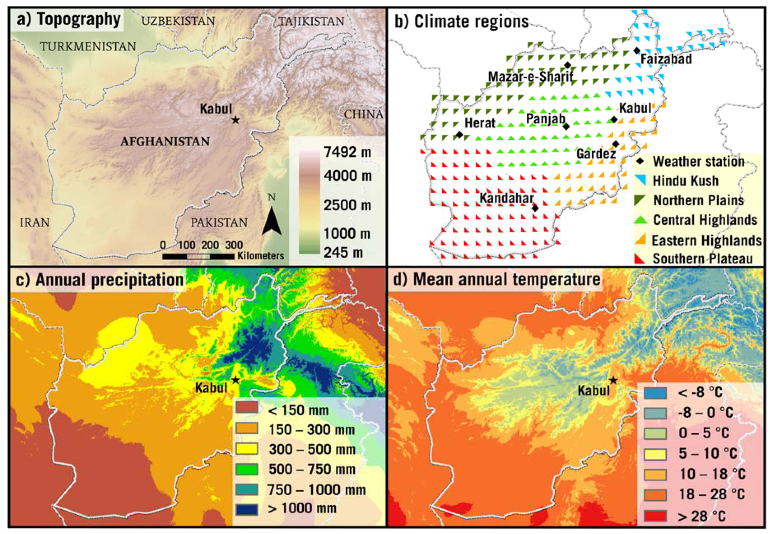
The geography of Afghanistan is dominated by the Hindu Kush mountain range, which runs from northeast to southwest and divides the country into different natural regions [31,32]. The variation in climate (Table 1), soil, topography, vegetation and other geographic features are fundamental [33]. This pronounced geographic heterogeneity also creates very different conditions for livelihoods and agricultural systems. In order to account for this heterogeneity in the context of climate change, Afghanistan has been subdivided into five major regions, derived from the ecoregion zoning provided by the World Wildlife Fund [34] (Figure 1). The most important crop in all regions of Afghanistan is wheat (winter and spring) with a share of over 80% of total crop production. Regionally, various other crops as well as fruit crops are grown [5]. In the following sections, the climate, overall geography, and the main agricultural features of each region are summarized.

2.1.1. Hindu Kush

The Hindu Kush region in the Northwest is mainly covered by Badakhshan province, which also comprises the Wakhan corridor, including parts of the Pamir and Karakoram regions (~45,000 km2) [5]. The region has a population of around one million people, with only around 4% living in urban areas [5]. It is the highest and most mountainous part of Afghanistan with over three-quarters of its area covered with mountains [35]. It receives the highest amount of precipitation and approximately 7.5% of the land is covered with permanent snow and ice. Therefore, the Hindu Kush region is a major water source, feeding main rivers like the Amu Darya [36]. The vegetation of the region is mainly dominated by rangelands (>60%) while less than 1% of the total area is covered by forests and shrubs [36]. In total, 8.5% of the region is suitable for agricultural production [36], which is mainly used for the cultivation of wheat, alongside smaller areas of barley, maize, and fruit crops [5]. Due to its mountainous topography, the region is particularly prone to natural disasters such as landslides, avalanches, floods, flashfloods, and substantial erosion of fertile soil [4].

2.1.2. Northern Plains (North)

The Northern Plains (North) have a mean altitude of around 600 m covering around 30% of Afghanistan (~190,000 km2) [5]. This region has political and geographical importance because it links Afghanistan to Central and West Asia. Only about 20% of the nine million people living in the North reside in urban areas [5]. It is mainly covered by rangelands (~50%) and barren lands (~15%). Rain-fed agriculture is predominant (16.4%), while only about 7% of the land is available for irrigated agriculture [36]. The North is also called the food basket of the country as it produces a wealth of grain crops such as rice, wheat, barley and maize as well as fruit crops such as peaches, almonds, pomegranates, apples and grapes. In addition, in the North, saffron and cotton are produced [5]. The Northern Plains are also home to the Northern Pistachio Belt, one of the largest forest systems in the country, as well as of the most extensive flatlands of the country around the foothills of the Amu Darya River [37].

2.1.3. Central Highlands (Centre)

The Central Highlands in the middle of Afghanistan are characterized by deep valleys and mountain ranges of up to 6400 m. They cover around 20% of Afghanistan (~ 125,000 km2) [36]. Over 40% of the population in the region lives in urban areas [5]. The Central Highlands region is mainly covered by rangeland (>80%) and barren lands (~8%). Agriculture is predominantly irrigated (6%), though a small amount is still rain-fed (2%) [36]. Due to the mountainous nature of the Central Highlands, agriculture is mostly small scale. Other grown crops beside wheat are barley, maize and fruit crops [36].

2.1.4. Eastern Highlands (East)

The Eastern Highlands represent the smallest region of the country, covering around 11% of Afghanistan’s land (~72,000 km2). Here around 7% of the population lives in urban areas [5]. The Eastern Highlands regions consist mainly of rangelands (>56%), and the largest existing forests in the so-called Eastern Forest Complex (17%) can be found here. The Eastern Highlands is the only region that is directly influenced by the moist air masses of the Indian monsoon getting trapped at the high mountain slopes and bringing rain. Therefore, it is covered by forests and highly suitable for agriculture. The rains, however, also can cause flooding and land/mud slides. Agriculture is mainly irrigated, focusing on wheat and other crops [36].

2.1.5. Southern Plateau (South)

The Southern Plateau is the largest region and mainly covered by arid desert, with only the river and marshland areas viable for agriculture. The Helmand River divides the region and nourishes Lake Helmand. This region is also prone to sand and dust storms, mainly associated with northerly winds. The southern region covers around one-third of Afghanistan (~215,000 km2). Less than 20% of the population in the region lives in urban areas [5]. The Southern Plateau is mainly covered by barren land (>50%), rangeland (~20%), and sand (~15%). Agriculture is relatively small and always irrigated, covering only around 5% [36]. Although the southern region is the driest in the country, it still produces wheat and other crops and in some areas fruits [5].

2.2. Climate Data

The analysis of climate change and its impacts in Afghanistan for the past and the future are based on reanalysis and regional climate models (RCM) which were tested with the available but limited number of station data. The different data types are explained in the following sections.

2.2.1. Availability of Direct Meteorological Observations

Observed weather data is scarce in Afghanistan due to the limited number of meteorological stations and the political instability over the last four decades. In particular, under the Taliban regime data records were destroyed and observations stopped completely. Thus, an analysis of past climate purely based on station data would be unsatisfactory; therefore, reanalysis data is used additionally. In order to verify the reliability of the reanalysis data and also to validate the capability of the climate models to capture main characteristics of Afghanistan’s climate, observed data has been used. Historic data sets have been restored by the Project for the Promotion and Enhancement of the Afghan Capacity for Effective Development (PEACE) project [7] and are publicly available, however only on a monthly basis. Daily data for all of the few stations is incomplete and cannot be used as time series. Therefore, daily dynamics could not be validated, which has implications especially on the uncertainty of the extremes and will be considered in the discussion. The most complete monthly time series for each of the five climate regions and additionally for Kabul have been used to validate the reanalysis and the climate models for this analysis (Table 2, Figure 2).

2.2.2. Reanalysis Data

Due to the limited availability of station data (see Section 2.2.1), reanalysis data was used to analyze the climate of the second half of the 20th century until 2010. Climate reanalyses are numerical descriptions of the past climate. They are produced by assimilating all available observations in a weather forecast model. In this study, different reanalysis data products have been evaluated against station data for Afghanistan Water and global Change (WATCH) (WATCH Forcing Data 20th Century (WATCH; 1950–2001) [39], data from the Global Soil Wetness Project Phase 3 (GSWP3; 1901–2010) [40,41], and from the second version of the Global Meteorological Forcing Dataset for land surface modeling of Princeton University (PFGv2; 1901–2012) [42]; see Figure S1, supplementary material). They all showed comparable performances. ERA-Interim (1979–2012) [43] data is only available after 1979 and had therefore no overlap with the available observation periods (Table 2). WATCH showed good performance, however is not available continuously for the complete period of interest (from 1950 to 2010). GSWP3 has been selected due to its overall good performance over Afghanistan and its temporal coverage of the period from 1950 until 2010. It is generated globally on a 0.5° × 0.5° grid and provides amongst other parameters temperature at surface and precipitation at a daily time step.
The data is validated in order to estimate the robustness of the results. For this validation, the reanalysis data is compared to observed data of weather stations of the same time span (Table 2) in different regions of Afghanistan, where long time series are available (see Section 2.2.1). Since the data is on a 0.5° × 0.5° grid, the nine nearest tiles around the point have been averaged (9-point filter). This is a standard procedure in order to account for slight spatial shifts in the reanalysis grid [44,45]. The area of the compared data therefore has a mean of around 24,000 km2, and the regional geographical setting of the weather station, including its altitude, is therefore not reflected adequately. Still, the general physical patterns should be reproduced by the reanalysis but the absolute magnitudes of temperature and precipitation might differ.

2.2.3. Climate Projections

Climate projections from the Coordinated Regional Downscaling Experiment for South Asia (CORDEX-SA) have been used in this study [46]. CORDEX is an internationally coordinated framework to produce an improved generation of regional climate change projections world-wide, providing input for impact and adaptation studies. CORDEX data is provided for different domains around the globe. The South Asian domain covers all of Afghanistan. In total, 12 Earth system model—regional climate model (RCM) combinations are available and used in this study (Table 3). The data is gridded on a 0.5° × 0.5° mash and for Afghanistan it comprises over 300 tiles, which allows a detailed spatial analysis, especially for the mountainous areas of the Hindu Kush.
All model output covers at least the timespan from 1976 to 2099, of which the period until 2005 is the reference period. The scenarios start in the year 2006 with different available Representative Concentration Pathways (RCPs). The RCPs are named after the level of additional radiative forcing achieved by 2100, with respect to the pre-industrial value. For this study, RCP 4.5 and RCP 8.5 have been selected since they represent the realistic range from a reduction of greenhouse gas (GHG) emissions in the medium-term future (4.5) to a further increase in a business-as-usual scenario (8.5). RCP 4.5 corresponds to a low stabilization scenario, whereby in 2100 the radiative forcing is 4.5 W above the pre-industrial level. RCP 8.5 corresponds to a high-end scenario, whereby in 2100 the radiative forcing is 8.5 W above the pre-industrial level. RCP 4.5 corresponds to likely global warming of between 1.1 °C and 2.6 °C until the end of this century with respect to the pre-industrial level, and under the RCP 8.5 scenarios global temperatures are projected to increase between 2.6 °C to 4.8 °C [47].
The historical period of the CORDEX-SA data have been tested for the complete domain and with a focus on the summer monsoon [48,49] in order to assess their capability of reproducing the climate in the region. In general, they showed at least adequate performance. For Afghanistan, the performance of the models is evaluated in detail in order to estimate the level of reliability/uncertainty of the projections. For the validation, the historical period of the projections are interpolated to the weather stations, similarly to the procedure of the reanalysis. Since the historical runs of the models are not intended to reproduce the correct weather sequence but only the climate in the long run, the mean of the period from 1970 until 1999 has been used for the comparison instead of using the same time span as for the observations.

2.3. Indices and Statistical Methods

2.3.1. Indices

In order to not only capture the basic parameters of temperature and precipitation, but to account for climatic constraints of livelihood in Afghanistan, five additional parameters or indices are investigated: two for extremes (heavy precipitation, HWMI) and three that are especially relevant for Afghanistan’s agriculture (spring precipitation, Standardized SPEI, and growing GSL). For the preparation of the data and the calculation and processing of these seven parameters the R statistical software has been used [50]. In the following sections, the five additional parameters are briefly described.
Heavy precipitation leads to flash floods that occur regularly in Afghanistan. In addition, it causes substantial erosion, which already harms Afghanistan’s agriculture, destroys infrastructure and spreads epidemic diseases especially in degraded regions with strong relief energy such as in the north, Central Highlands, east and in the Hindu Kush [51]. Relevant months for these kinds of events are mainly March to September. Hence, the analysis for heavy precipitation is limited to these months. It is analyzed as the 95th percentile of days above 1 mm precipitation. This is a standard indicator for precipitation extremes and is used, for example, by the European Union [52].
Due to its continentality and the location in low latitudes, summer temperatures can be extreme in Afghanistan, especially in the regions with less elevation in the South and North. Here heat waves occur that affect human health and hinder physical labor and, hence, the economy of the mainly agricultural country with temperatures well above 40 °C for several days [51]. For quantifying heat waves, several approaches and indices exist. The HWMI was chosen for this study since it takes into account both magnitude and duration of the heat waves and has been successfully applied for analyzing future climate projections [53]. It is defined as the maximum of the heat waves in a year with at least three consecutive days above the threshold for the reference period 1981–2010. The threshold is calculated as 90th percentile of daily maxima, centered on a 31-day window. The HWMI is classified into seven categories: 1–2: normal, 2–3: moderate, 3–4: severe, 4–8: extreme, 8–16: very extreme, 16–32: super extreme and above 32 ultra-extreme. The process is described in detail in Russo et al. (2014) [53]. The dimensionless HWMI was calculated using the R package “extRemes” [54].
The SPEI is an advanced version of the Standardized Precipitation Index and takes into account not only precipitation but also potential evapotranspiration (PET) [55]. The SPEI uses the difference between precipitation and PET to calculate a simple climatic water balance. It is standardized using a log-logistic distribution and has a standard deviation of 1 [56,57]. An SPEI of 0 indicates a value corresponding to 50% of the cumulative probability. Positive values indicate above average moisture conditions and negative values indicate dry conditions. According to the scale used for the common Standard Precipitation Index, values between −1.00 and −1.99 represent extremely dry conditions and those exceeding −2.00 represent severely dry conditions. Both the SPEI and the potential evapotranspiration (PET) have been calculated on a monthly basis using the R package “SPEI” [55]. PET is estimated using the Thornwaite equation [58] which is based on monthly average temperature and latitude. The procedure to calculate the index is complex and involves a climatic water balance and adjustment to a log-logistic probability distribution. For this study a 12-month accumulation period is used for the analysis. The normalization period for the reanalysis was set to 1951 to 1980 and for the scenarios to 1976 to 2005.
Spring precipitation is especially important for rain-fed crop cultivation in Afghanistan, which is still the dominant form of agriculture [59]. January to April have been identified as relevant months for this important rainfall period and the parameter is calculated accordingly as the mean of these four months [60].
GSL is a standard index defined by the Expert Team on Climate Change Detection and Indices of the World Meteorological Organization [61,62]. It counts the days between first span of at least six days with daily mean temperature above 5 °C and the first span after July 1 of six days with mean temperature below 5 °C of a year. Above this temperature threshold, growth of crops is generally possible.

2.3.2. Analysis of Trends and Changes

Linear trends in the time series or indices based on means (annual mean temperature, annual precipitation, spring precipitation, SPEI, and GSL) were identified using the Mann–Kendall test [63]. For this robust nonparametric test, each element is compared with its successors and ranked as larger, equal, or smaller. Based on this analysis the statistical significance of rejecting the null hypothesis that there is no monotonic trend is tested (for all tests α = 0.05). The R package “Kendall” was used for the calculation [64].
In order to quantify the linear trend the Theil–Sen approach was used [65,66]. It is commonly used with the Mann–Kendall test and estimates the trend slope of a time series in its original unit. The R package “zyp” was used to calculate the Theil–Sen trend and includes a pre-whitening according to Ye et al. (2002) [67] if autocorrelation occurs [68].
For trends in extremes (heavy precipitation and HWMI) the well-established method of quantile regression is used [69]. In contrast to classic regression that estimates the conditional mean of a predictand’s distribution on the basis of one or more predictors, quantile regression is a more generalized linear approach that estimates the median or any given quantile of the predictand [70]. Mathematically, quantile regression requires a more complex optimization algorithm based on linear programming than the least-square fit used in classic linear regression. For this study, the R package “quantreg” was used to estimate the trend and its significance (for all tests α = 0.05) [71].
To analyse the changes between the period 1951 to 1980 and 1981 to 2010, difference maps are used. The changes are statistically tested with a t-test for independent samples for every grid bix (α = 0.05).

3. Results

3.1. Validation of Reanalysis

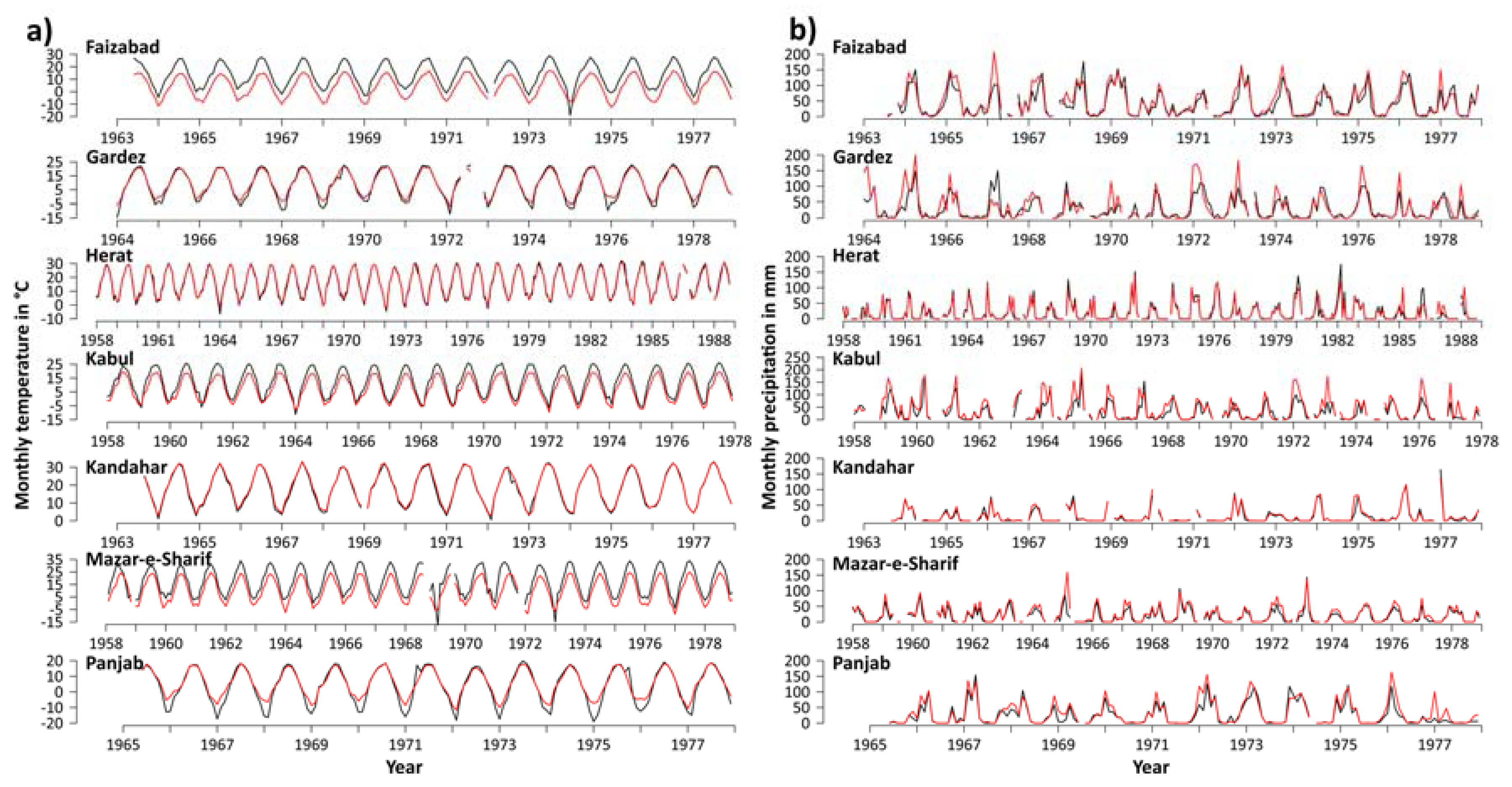
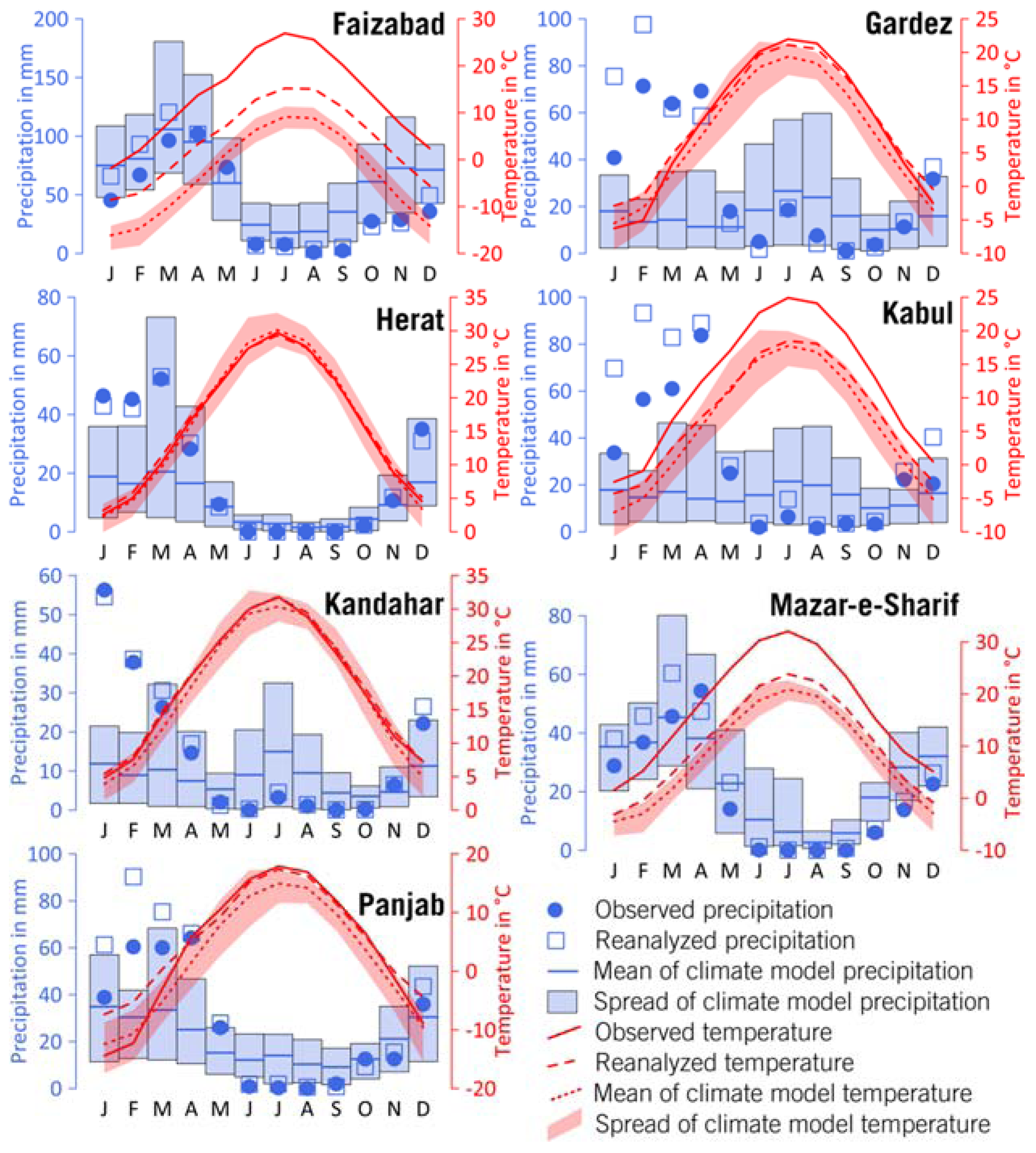
The validation of the reanalysis and historical model data is done based on monthly time series and in a qualitative way (Figure 3 and Figure 4); the results and their implications on uncertainty are discussed in Section 4.1. The seasonal variations of temperatures of the reanalysis data are in good agreement with meteorological measurements at all stations. The absolute magnitudes of temperatures are well reflected for Gardez (East), Herat (Northwest), Kandahar (South), and mostly for Panjab (Center). For Faizabad (Hindu Kush), Mazar-e Sharif (North), Kabul and partly Panjab (Centre) the absolute magnitudes differ. However, for Faizabad, the reanalyzed and monthly averaged temperatures are underestimated by approximately 5 °C and for Mazar-e Sharif and Kabul by approximately 3 °C to 5 °C. For Panjab, the winter temperatures are underestimated by approximately 5 °C. These differences are discussed in Section 4.1.
The seasonal cycle for precipitation is generally correct for all stations with one rainy season in the North during winter and spring and for the stations in the East that are influenced by the summer monsoon, an additional small rainy season occurs in summer (Gardez, Kabul, Kandahar). In terms of absolute monthly magnitudes, Herat (North) and Kandahar (South) are well in line with observations during all months. For the other five stations, monthly precipitation between May and December is reasonably estimated. Precipitation between January and April for these stations is, however, mainly overestimated by up to approximately 40 mm in some cases.

3.2. Performance of Climate Models

The comparison between the historical climate model runs and observations shows similar patterns for temperature even though for some stations the absolute temperature level differs. The models are able to reproduce the seasonal temperature cycle for all stations. The absolute values of model mean and the simulated range of monthly temperature are in the same ranges as in the observations for all stations except for Faizabad, Mazar-e Sharif and Kabul. Here the deviations range in the same order of magnitude as in the reanalysis. This is further discussed in Section 4.1.
With respect to precipitation, the results differ completely. Only for stations Faizabad, Mazar-e Sharif and partly for Herat in the northern part of Afghanistan are the models capable of reproducing the observed seasonal cycle of monthly precipitation. For all the other stations, the models particularly underestimate the spring precipitation from January to April. Only the onset of winter precipitation is simulated correctly for these stations; however, not the observed magnitudes. This has strong implications on the interpretability of these data which is discussed in detail in Section 4.1.

3.3. Analysis of Past Climate Trends for the Period 1951–2010

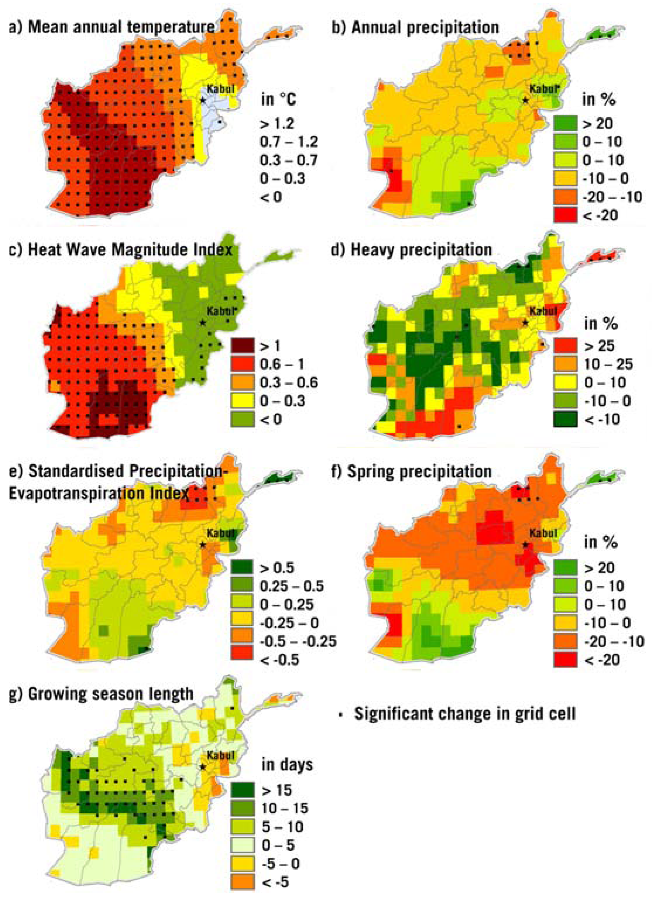
The general climatic trends are depicted in the Figure 5a,b and quantified for the regions in Table 4. In the reanalysis, the mean annual temperature increased substantially in most parts of Afghanistan by up to 1.2 °C in a diagonal northwest–southeast belt west of the Central Highlands for the difference between 1981/2010 and 1951/1980. The temperature for the whole period from 1951 to 2010 for all Afghanistan even increased by 1.8 °C, with highest increases of 2.4 °C in the east and only 0.6 °C in the Hindu Kush region. Towards the northeast and west, the temperature increase fades. No increase is detectable in the region southeast of Kabul. In Badakhshan, in the northeast, where Afghanistan’s main glaciered areas are located, the warming is between 0.3 and 0.7 °C. All these trends are statistically significant.
The trends in the reanalysis for annual precipitation are less distinct for most parts. In addition they are not significant for all regions. Most parts of Afghanistan experienced changes between −10% and +10%. Only in small areas in the North and the West, the decrease is up to −20% and partly above. In the Wakhan corridor in Badakhshan and in the small areas along the border to Pakistan, stronger precipitation increases are shown by the reanalysis.
Changes in HWMI are similar to mean annual temperature in northwest-southeast oriented bands. The highest increases of over 1 of the standardized index are located in the arid areas in the southeast. The increases in the North, Centre and South regions are significant for the period 1951–2010.
Heavy precipitation between March and September increased in the East along the border to Pakistan up to 25% and above. For most of the country, however, the reanalysis shows a decrease mainly in the North, the Central Highlands and the Southwest. The changes over the whole period from 1951 to 2010 are not significant.
In Figure 5e–g indices are plotted that are directly relevant for agriculture in Afghanistan. The SPEI indicates a decrease for most of Afghanistan, meaning an increase of drought frequency and magnitude in the past. The strongest changes are indicated for the northeastern part with a decrease of over 0.5, meaning more than half of the standard deviation. In the East smaller areas occur with an increase of SPEI, meaning a reduction of droughts. Still, none of the SPEI changes for the whole region is significant in the reanalysis data.
Spring precipitation (January to April) decreased in the northern regions and the Central Highlands of Afghanistan whereas for the southeastern part an increase is indicated. Again, averaged over the regions, the trends are not significant.
Significant GSL changes in Afghanistan extend especially along a northwest–southeast band, similar to the strongest heating. Here up to over 15 days of increase for the growing season is indicated by the reanalysis. For all of Afghanistan, from 1951 to 2010 the GSL significantly increased by over 12 days, even though it increased only by 2.8 days in the eastern region.
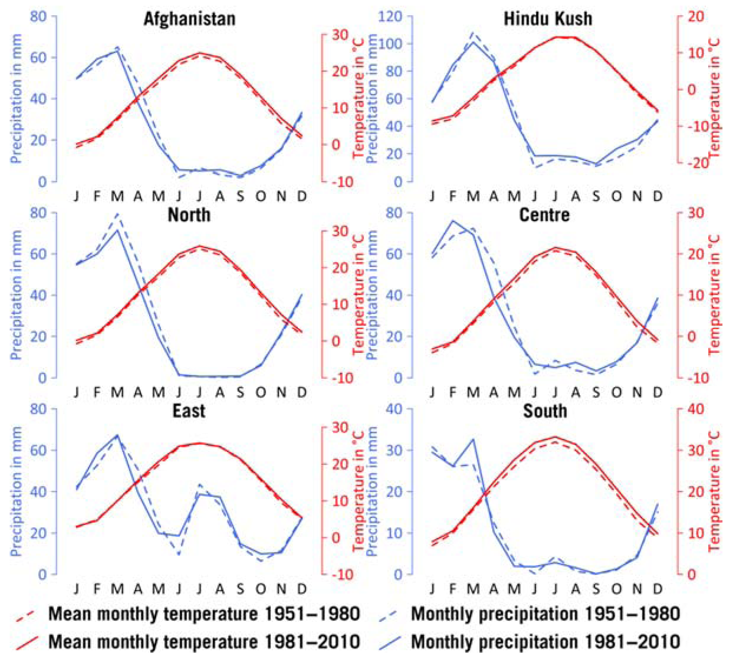
Changes in seasonality for monthly temperature and precipitation are depicted in Figure 6. With regard to temperature, there is no change in seasonality visible. Temperature increased rather uniformly throughout the whole year with lowest increases at the beginning of the calendar year.
Precipitation decreased for all Afghanistan and all regions, except for the South, from March to May, and increased slightly from around June to February. This implies a slight shift of the seasons towards an earlier onset of precipitations. This pattern is most apparent in the North and Centre. In the South, no general pattern can be described but an increase in March and, less distinct, summer monsoon precipitation in July.

3.4. Analysis of Future Climate Trends for the Time Period 2006–2050/2099

The future climate model projections are, similarly to the reanalysis, analyzed in two ways: the differences between the mean of a future period 2021/2050 and a base period 1976/2005 are mapped for the different parameters (Figure 7). In addition, linear trends are detected for the period 2006–2050 and 2006–2099 (Table 5).
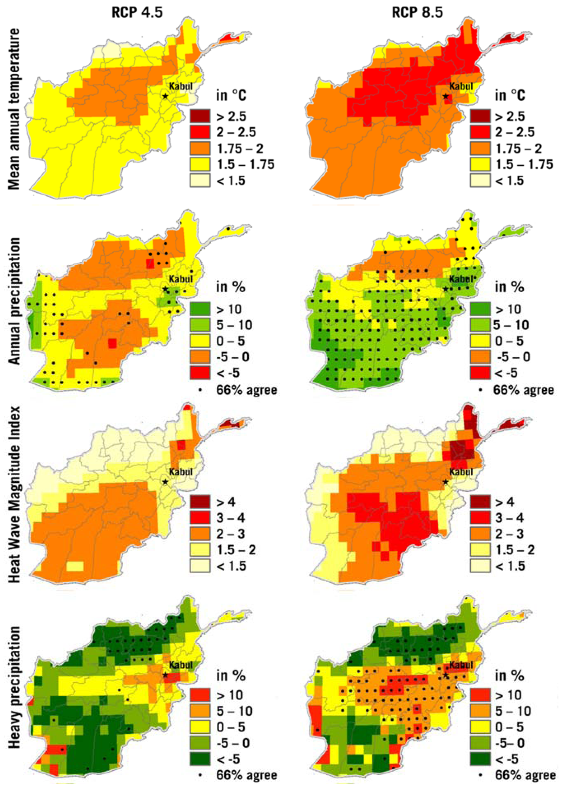
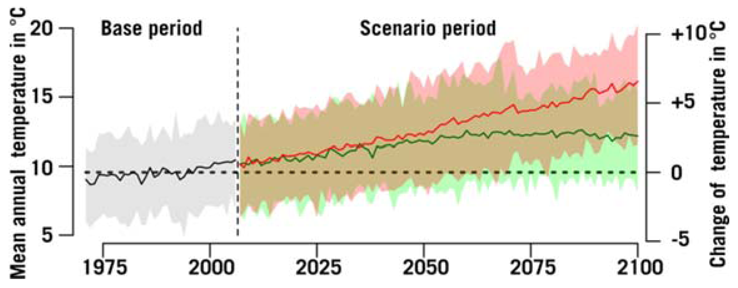
Mean annual temperature is projected to increase significantly when comparing the mean for the future period with the base period for all of Afghanistan and for all regions for the low emission scenario RCP 4.5 as well as for business-as-usual scenario RCP 8.5. For RCP 4.5, the strongest warming is in the Wakhan corridor with over 2 °C, followed by the Central Highlands with a warming of 1.75° to 2 °C. The other parts are projected to experience an increase of 1.5° to 1.7 °C. Under RCP 8.5, the spatial pattern is almost identical, however, with a magnitude that is generally 0.25 °C larger. Temperatures after 2050 until 2099 continue to increase under RCP 4.5 but less quickly. Under RCP 8.5 the warming, however, is projected to accelerate and reaches approximately 6 °C in most regions and in the Hindu Kush even over 7 °C until 2099 (Figure 8). The model spread and the related uncertainty for the models is approximately 5 °C with all models showing very similar degrees of relative warming. The ensemble mean is more or less in the middle of the ensemble spread, indicating a homogeneous distribution.
The changes of annual precipitation are small, ranging between −5% and + 10%. Only under RCP 8.5 is there a slight wetting trend of 5–10% projected for the South, the East, and the Centre by more than 66% of the models. Until 2050, the trends are not significant with the exception of RCP 8.5 in the North. Until 2099, the signal becomes clearer and most models indicate a decrease, which is significant under RCP 8.5 for the East, North, and the Centre. The model spread is large in relation to the average, underlining the large uncertainty of the precipitation projections.
HWMI is projected to increase by all models under both scenarios for all of Afghanistan. The mean increase over all models for the future period 2021/2050 is between 1 and over 4. Given the definition of category 4–8 as extreme heat wave, this increase is substantial. The strongest increases are in the Wakhan corridor, Hindu Kush, and a large hotspot of HWMI increase covers the Centre, South and East with increases of 2–3 under RCP 4.5 and 2–4 under RCP 8.5. Until 2099, the projected increases under RCP 8.5 are enormous with +8.5 for all of Afghanistan and even 12 for the Hindu Kush region alone.
For heavy precipitation between March and September, the projected signals from the models are spatially incoherent, similar to annual precipitation. In the East and the Central Highlands, the ensemble mean indicates an increase by up to 10%. For the other parts of the country slight decreases are projected. Under RCP 4.5 there is almost no agreement among the models in terms of the trend and for RCP 8.5 over 66% of the models agree for the projected increase in the Centre. The regional trends until 2099 are similar but with even higher uncertainties and none of the regional trends of the model ensemble is significant.
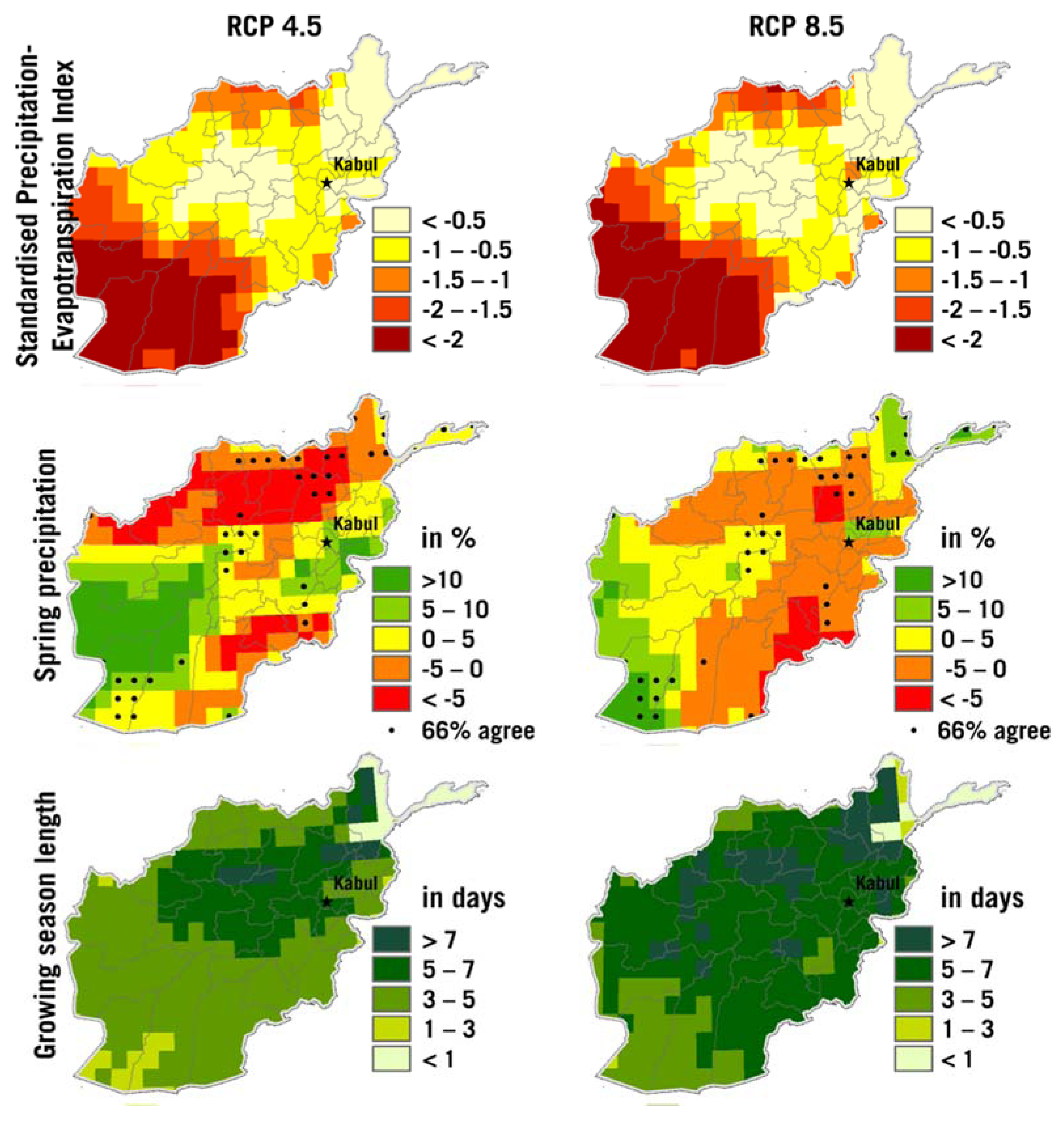
The results of the analysis of the agriculturally relevant parameters are presented in Figure 9 and Table 6. The SPEI difference maps show a strong decrease in southern Afghanistan by over 2 standard deviations, meaning a strong increase in drought. In the other parts of the country, the SPEI is projected to decrease mainly by 1 to 0.5, and slightly below. All trends are significant but for the Hindu Kush. The differences between the scenarios until 2050 are small. The trends until 2090, however, reveal an intensification of droughts under RCP 8.5 by −2.32 for the mean of all Afghanistan. All trends under the RCP 4.5 scenario are also significant. For the future, the pattern of change of SPEI does not agree with the patterns of temperature or precipitation change. The non-linear increasing evaporation with increasing temperature can explain this effect. The smaller increase in temperature in the hot South and West of Afghanistan has a stronger effect on the evaporation (due to high absolute temperature values) compared the stronger increase in the central highlands, where absolute temperatures are, however, still lower.
The projected changes for spring precipitation are rather small between −5 to +10% and the patterns are heterogeneous. The models hardly agree in the direction of the trends, only in the North there is some agreement with respect to a small decrease of desertification in spring. The differences between the scenarios are small. Until 2099, most models show a decrease in precipitation which is significant under the RCP 8.5 scenario in all regions and in the mean for Afghanistan this decrease amounts to more than 30%. Still, the model spread is large and some models project an increase of spring precipitation.
In contrast, the signal for GSL is very obvious and significant for all regions under both scenarios and time periods. The growing season across all regions of Afghanistan, especially the central part, is projected to increase by 7 days until 2050 compared to the base period. Under RCP 8.5, the trends in all regions until 2099 are especially extreme and for the whole of Afghanistan the ensemble mean projects an increase of nearly 60 days.
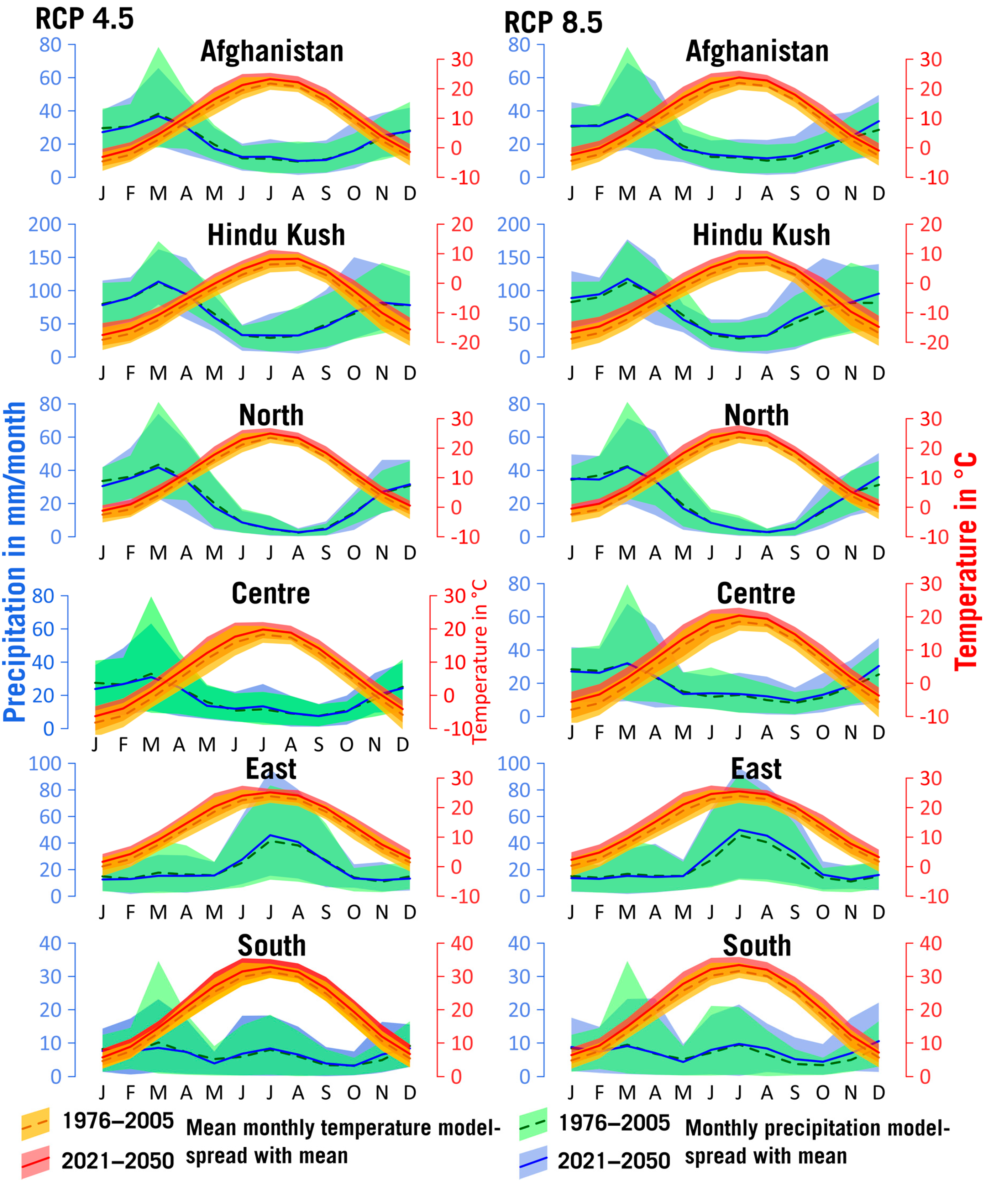
The projected changes in the seasonality of temperature and precipitation are illustrated in the climate diagrams in Figure 10 for the period from 2021 and 2050 and in the supplementary material in Figure S2 for the future period 2070–2099. The projected temperature increase is, similar to the observations, homogeneous throughout the year. With regard to precipitation, there is a slight shift to an earlier onset of the rainy season for all regions, which is more pronounced under RCP 8.5 than under RCP 4.5.

4. Discussion and Conclusions

4.1. Robustness and Uncertainties of the Results

The validation using the 9-point filter or other interpolation-to-point techniques are inherently problematic. In this study, the area of the compared data of the nine grid cells is the mean of around 24,000 km2. The regional geographical setting of the weather station, including its altitude, is therefore not reflected adequately. The general physical patterns should be reproduced by the reanalysis but the magnitudes of local temperature and precipitation might differ, e.g., due to topographic characteristics of the weather station. For example, Faizabad is located in the Kokcha valley (Figure 2). Due to this lower location, temperatures are distinctly warmer than the mean of the surrounding mountainous area. Therefore, the temperature difference between the reanalysis and the measurements vary strongly but still show the same seasonal cycle. For stations in less orographic terrain, such as Kandahar, Herat and Gardez, the validation shows a more adequate performance, observed and reanalyzed temperatures being almost equal. This means that in terms of temperature, the reanalysis data at its given scale is quite reliable.
In terms of precipitation, regional differences are larger and the results are more heterogeneous, e.g., throughout the seasonal cycle. For the stations in mountainous areas, the described effect of the 9-point-filter is apparent. In addition, climate and weather models still have difficulties with high altitudes, since the spatial resolution of the cells is often too coarse to represent relevant processes that lead to rainfall at station locations. This bias is stable during the whole period. As mainly relative changes are considered for the analysis of precipitation, there is also some agreement between reanalysis and station data. Especially heavy precipitation from the reanalysis could not be validated with station data because the latter are marked by large gap.
For the regional climate model data, the same difficulties apply as for the reanalysis and additional sources of uncertainty come along. Nevertheless, the simulated seasonal cycle of temperature seems reliable. This holds for all derived parameters and indices, i.e., annual mean temperature, HWMI, SPEI, and GSL. In contrast, precipitation and the related indices that are mainly based on precipitation (i.e., annual precipitation, heavy precipitation and spring precipitation) are partly not satisfactorily reproduced by the models. In the East, the North, and the Hindu Kush, the general patterns are well represented. In contrast, the precipitation validation in the Centre and the South are, especially during spring, less promising: the models are not able to reproduce the basic patterns and, therefore, the results for these regions should not be included in the interpretation and discussion.
In summary this means that temperature and related indices (mean annual temperature, SPEI, HWMI, GSL), as well as monthly precipitation and related parameters (annual precipitation, spring precipitation) are more reliable from reanalyses compared to the sparse station data. In contrast, the performance of the GSWP3 in terms of precipitation extremes reanalysis could not be assessed, since no daily data for the validation was available. Concerning the CORDEX-SA simulations, temperature and the related indices again are reliable. For precipitation, the results of annual and spring precipitation are satisfactory in the East and North, but they are not in the Centre and South of Afghanistan.
This partly discouraging result implies a strong need for an improvement of current observations, including the potential rescue and restoration of currently unused data. It is likely that there are more analogue observations of weather stations which are currently not available due to malfunctioning administration in the responsible national ministries/agencies. With a relatively small effort, large improvements in regard of a better understanding of past climate variations and changes could be achieved, which would also help to improve current models for the future. Another option might be the exploitation of existing remote sensing data. In this regard international research has treated Afghanistan poorly and there is still a huge potential for research.

4.2. Climate Impacts

The observed and projected climatic changes found in this study tell a fairly coherent story, although there is large uncertainty with regard to precipitation. In the past, the changes are mainly characterized by temperature increases and, no matter in which direction precipitation goes, temperature increases will certainly affect ecosystems and livelihood in Afghanistan. These changes have already begun and Afghanistan has experienced a temperature increase substantially higher than in the global mean, amounting to 1.8 °C between 1951 and 2010. This warming is projected to continue from 2006 until 2050 by 1.7–2.3 °C and afterwards even 2.7–6.4 °C until 2099 across the whole country. The range is determined by the amount of global emissions. This is in accordance with the overall regional results for Central Asia which, depending on the emission scenario, are projected to be 2.5 °C compared with 2 °C globally and even 6.5 °C compared with a 4 °C global warming until the end of the century [7]. The effects of unprecedented heat waves, as indicated by the HWMI results, will directly affect the health sector in Afghanistan. Projected increases by 8 to 16 mean that Afghanistan will regularly experience very extreme heat waves, especially under the business-as-usual emission scenario RCP 8.5. Temperature will also impact on water resources and agriculture as well as on natural ecosystems in Afghanistan. Increasing evapotranspiration as indicated by the SPEI will probably exacerbate the country’s already difficult conditions.
Although Afghanistan has vast water resources (approximately 1700 m3 per capita per year, which in theory is sufficient for domestic, agricultural, industrial, and environmental needs), the country still does not use the resources efficiently due to a lack of water management capacity in the face of the large regional as well as intra- and interannual variability of water availability [72]. In the future, this situation may become even more problematic given the growing demand related to population growth, economic development, and improved standards of living. Despite Afghanistan’s strong dependency on agriculture, which employs around 85 percent of the population directly or indirectly and contributes around 30% to the gross domestic product [72], only very few research and impact studies for agriculture and water resources have been conducted (see Section 1). Only the glaciers of the Hindu Kush have attracted the attention of some international research activities [13,14,16,17,18,20].
The negative impacts of climate change not only hold for the agricultural sector but also for Afghanistan’s natural ecosystems, which have already been deteriorated during the country’s many years of conflict, unsustainable management, and over-exploitation. For example, over 80% of Afghanistan’s land is said to be subject to soil erosion [36]. This discussion can also be extended for the hazard landscape of Afghanistan. The numerous regularly occurring hazards like avalanches, floods, droughts, landslides but also long-term erosion are related to the changing climate [73]. Also in this regard, there is a large research deficit for Afghanistan. The contribution of this study to hazard research is limited due to its more general character; however, it is likely that droughts will occur more often and hazards related to runoff, such as landslides, floods and flash floods, are likely to be enhanced by climate change [74,75].
Overall, the current results show that in addition to the already existing deficit in adaptation to current climate conditions, the situation will be aggravated in the future, particularly in the areas of water management and agriculture. Thus, the results of this study underline the importance of adaptation to climate change in Afghanistan.
This holds even more because there is also a clear positive signal in the results. The GSL will increase substantially with rising temperatures, e.g., by around 20 days on average until 2050. This might open the opportunity for extended agricultural usage or in some cases even an additional harvest. This requires, of course, a smart management of water resources and a more sophisticated and climate-adapted agriculture.

Supplementary Materials

Supplementary materials can be found at www.mdpi.com/2225-1154/5/2/38/s1. Figure S1: Validation of long-term monthly mean temperature and monhtly mean precipitaion of three reanalysis products (Global Soil Wetness Project Phase 3 (GSWP3), WATCH Forcing Data 20th Century (WATCH), second version of the Global Meteorological Forcing Dataset for land surface modeling of Princeton University (PFGv2)) against observation data for one weather station in each of the six climate regions of Afghanistan and Kabul (Figure 1) (see Section 2.2.2 for periods). Figure S2: Projected changes of seasonality for temperature and precipitation as monthly values for the periods 1976–2005 and 2070–2099 for all Afghanistan and five climate regions for Representative Concentration Pathways 4.5 and 8.5.

Acknowledgments

We thank the CORDEX community for producing and sharing the regional climate projections.

Author Contributions

Valentin Aich designed the study, analyzed the data. All authors wrote the paper.

Conflicts of Interest

The authors declare no conflict of interest.

References

  1. Kreft, S.; Eckstein, D.; Dorsch, L.; Fischer, L. Global Climate Risk Index 2016: Who Suffers Most from Extreme Weather Events? Weather-Related Loss Events in 2014 and 1995 to 2014; Germanwatch: Bonn, Germany, 2015. [Google Scholar]
  2. University of Notre Dame Afghanistan Notre Dame Global Adaptation Index. Available online: http://index.gain.org/country/afghanistan (accessed on 1 February 2017).
  3. Maplecroft. Climate Change Risk Atlas 2011. Available online: https://maplecroft.com/about/news/ccvi.html (accessed on 1 February 2017).
  4. UNEP. Afghanistan Post-Conflict Environmental Assessment; UNEP: Kabul, Afghanistan, 2003. [Google Scholar]
  5. Central Statistical Office. Afghanistan Statistical Yearbook 2015–2016. Available online: www.emdat.be (accessed on 1 July 2017).
  6. EM-DAT The OFDA/CRED International Disaster Database. Available online: www.emdat.be (accessed on 1 July 2015).
  7. World Bank. Turn Down the Heat: Confronting the New Climate Normal; World Bank: Washington, DC, USA, 2014. [Google Scholar]
  8. McSweeney, C.; New, M.; Lizcano, G.; Lu, X. The UNDP climate change country profiles, Improving the accessibility of observed and projected climate information for studies of climate change in developing countries 2010. Am. Meteorol. Soc. 2010, 157–166. [Google Scholar] [CrossRef]
  9. Savage, M.; Dougherty, B.; Hamza, M.; Butterfiled, R.; Bharwani, S. Socio-Economic Impacts of Climate Change in Afghanistan; Stockholm Environment Institute: Oxford, UK, 2009. [Google Scholar]
  10. Ridley, J.; Wiltshire, A.; Mathison, C. More frequent occurrence of westerly disturbances in Karakoram up to 2100. Sci. Total Environ. 2013, 468–469, S31–S35. [Google Scholar] [CrossRef] [PubMed]
  11. Mukhopadhyay, B.; Khan, A. A quantitative assessment of the genetic sources of the hydrologic flow regimes in Upper Indus Basin and its significance in a changing climate. J. Hydrol. 2014, 509, 549–572. [Google Scholar] [CrossRef]
  12. Ososkova, T.; Gorelkin, N.; Chub, V. Water Resources of Central Asia and Adaptation Measures for Climate Change. Environ. Monit. Assess. 2000, 61, 161–166. [Google Scholar] [CrossRef]
  13. Unger-Shayesteh, K.; Vorogushyn, S.; Farinotti, D. What do we know about past changes in the water cycle of Central Asian headwaters? A review. Glob. Planet. Chang. 2013, 110, 4–25. [Google Scholar] [CrossRef]
  14. Hagg, W.; Hoelzle, M.; Wagner, S.; Mayr, E. Glacier and runoff changes in the Rukhk catchment, upper Amu-Darya basin until 2050. Glob. Planet. Chang. 2013, 110, 62–73. [Google Scholar] [CrossRef]
  15. Dukhovny, V.; de Schutter, J. Water in Central Asia: Past, Present and Future; CRC Press: New York, NY, USA, 2011. [Google Scholar]
  16. Radić, V.; Bliss, A.; Beedlow, A.C.; Hock, R.; Miles, E.; Cogley, J.G. Regional and global projections of twenty-first century glacier mass changes in response to climate scenarios from global climate models. Clim. Dyn. 2014, 42, 37–58. [Google Scholar] [CrossRef]
  17. Bliss, A.; Hock, R.; Radić, V. Global response of glacier runoff to twenty-first century climate change. J. Geophys. Res. Earth Surf. 2014, 119, 717–730. [Google Scholar] [CrossRef]
  18. Marzeion, B.; Jarosch, A.H.; Hofer, M. Past and future sea-level change from the surface mass balance of glaciers. Cryosph. Discuss. 2012, 6, 3177–3241. [Google Scholar] [CrossRef]
  19. Siegfried, T.; Bernauer, T.; Guiennet, R.; Sellars, S.; Robertson, A.W.; Mankin, J.; Bauer-Gottwein, P.; Yakovlev, A. Will climate change exacerbate water stress in Central Asia? Clim. Chang. 2012, 112, 881–899. [Google Scholar] [CrossRef]
  20. Lutz, A.; Immerzeel, W.; Gobiet, A. Comparison of climate change signals in CMIP3 and CMIP5 multi-model ensembles and implications for Central Asian glaciers. Hydrol. Earth Syst. Sci. 2013, 17, 3661–3677. [Google Scholar] [CrossRef]
  21. Wiltshire, A.J. Climate change implications for the glaciers of the Hindu Kush, Karakoram and Himalayan region. Cryosphere 2014, 8, 941–958. [Google Scholar] [CrossRef]
  22. Jarsjö, J.; Asokan, S.M.; Prieto, C.; Bring, A.; Destouni, G. Hydrological responses to climate change conditioned by historic alterations of land-use and water-use. Hydrol. Earth Syst. Sci 2012, 16, 1335–1347. [Google Scholar] [CrossRef]
  23. Shibuo, Y.; Jarsjö, J.; Destouni, G. Hydrological responses to climate change and irrigation in the Aral Sea drainage basin. Geophys. Res. Lett. 2007, 34, L21406. [Google Scholar] [CrossRef]
  24. Jaramillo, F.; Destouni, G. Local flow regulation and irrigation raise global human water consumption and footprint. Science 2015, 350, 1248–1251. [Google Scholar] [CrossRef] [PubMed]
  25. Hagen, E.; Teufert, J.F. Flooding in Afghanistan: A Crisis; Springer: Dordrecht, The Netherlands, 2009; pp. 179–185. [Google Scholar]
  26. Hagen, E.; Shroder, J.F.; Lu, X.X.; Teufert, J.F. Reverse engineered flood hazard mapping in Afghanistan: A parsimonious flood map model for developing countries. Quat. Int. 2010, 226, 82–91. [Google Scholar] [CrossRef]
  27. Shroder, J.F.; Weihs, B.J.; Schettler, M.J. Mass movement in northeast Afghanistan. Phys. Chem. Earth Parts A/B/C 2011, 36, 1267–1286. [Google Scholar] [CrossRef]
  28. Azimi, A. Environment Assessment for ADB’s Program in Afghanistan; Country Partnership Strategy: Kabul, Afghanistan, 2007. [Google Scholar]
  29. UNEP; National Environmental Protection Agency of Afghanistan (NEPA). Afghnaistan’s Environment 2008; UNEP: Kabul, Afghanistan, 2008. [Google Scholar]
  30. Bromand, M.T. Impact Assessment of Climate Change on Water Resources in the Kabul River Basin; Afghanistan, Ritsumeikan University: Shiga, Japan, 2015. [Google Scholar]
  31. Amin, H.; Schilz, G.B. A Geography of Afghanistan; University of Nebraska at Omaha: Omaha, NE, USA, 1976. [Google Scholar]
  32. Library of Congress-Federal Research Division. Country Profile: Afghanistan. Available online: https://www.loc.gov/rr/frd/cs/profiles/Afghanistan.pdf (accessed on 4 July 2017).
  33. Grötzbach, E. Afghanistan: Eine Geographische Landeskunde; Wissenschaftliche Buchgesellschaft: Darmstadt, Germany, 1990. [Google Scholar]
  34. Olson, D.M.; Dinerstein, E.; Wikramanayake, E.D.; Burgess, N.D.; Powell, G.V.N.; Underwood, E.C.; D’amico, J.A.; Itoua, I.; Strand, H.E.; Morrison, J.C.; et al. Terrestrial Ecoregions of the World: A New Map of Life on Earth. Bioscience 2001, 51, 933. [Google Scholar] [CrossRef]
  35. Ministry of Rural Rehabilitation & Development. National Area-Based Development Programme (NABDP)—Provincial Profile Badakshan; Ministry of Rural Rehabilitation & Development: Kabul, Afghanistan, 2014.
  36. FAO. Land Cover Atlas of the Islamic Republich of Afghanistan; FAO: Kabul, Afghanistan, 2016. [Google Scholar]
  37. Favre, R.; Kamal, G.M. Watershed Atlas of Afghanistan; FAO: Kabul, Afghanistan, 2004. [Google Scholar]
  38. Hijmans, R.J.; Cameron, S.E.; Parra, J.L.; Jones, P.G.; Jarvis, A. Very high resolution interpolated climate surfaces for global land areas. Int. J. Climatol. 2005, 25, 1965–1978. [Google Scholar] [CrossRef]
  39. Weedon, G.P.; Gomes, S.; Viterbo, P.; Shuttleworth, W.J.; Blyth, E.; Österle, H.; Adam, J.C.; Bellouin, N.; Boucher, O.; Best, M. Creation of the WATCH Forcing Data and Its Use to Assess Global and Regional Reference Crop Evaporation over Land during the Twentieth Century. J. Hydrometeorol. 2011, 12, 823–848. [Google Scholar] [CrossRef]
  40. Kim, H. GSWP3. Available online: http://hydro.iis.u-tokyo.ac.jp/GSWP3/exp1.html (accessed on 24 April 2015).
  41. Kim, H.; Yoshimura, K.; Chang, E.; Famiglietti, J.S.; Oki, T. Century long observation constrained global dynamic downscaling and hydrologic implication. Proceeding of the American Geophysical Union Fall Meeting 2012, San Francisco, CA, USA, 3–7 December 2012. [Google Scholar]
  42. Sheffield, J.; Goteti, G.; Wood, E.F. Development of a 50-year high-resolution global dataset of meteorological forcings for land surface modeling. J. Clim. 2006, 19, 3088–3111. [Google Scholar] [CrossRef]
  43. Weedon, G.P.; Balsamo, G.; Bellouin, N.; Gomes, S.; Best, M.J.; Viterbo, P. The WFDEI meteorological forcing data set: WATCH Forcing data methodology applied to ERA-Interim reanalysis data. Water Resour. Res. 2014, 50, 7505–7514. [Google Scholar] [CrossRef]
  44. Grasso, L.D. The differentiation between grid spacing and resolution and their application to numerical modeling. Bull. Am. Meteorol. Soc. 2000, 81, 579–580. [Google Scholar]
  45. Jacob, D.; Göttel, H.; Kotlarski, S.; Lorenz, P.; Sieck, K. Klimaauswirkungen und Anpassung in Deutschland–Phase 1: Erstellung regionaler Klimaszenarien für Deutschland. Clim. Chang. 2008, 11, 154. [Google Scholar]
  46. Jones, C.; Giorgi, F.; Asrar, G. The Coordinated Regional Downscaling Experiment: CORDEX—An international downscaling link to CMIP5. Clivar Exch. 2011, 16, 34–40. [Google Scholar]
  47. IPCC. Climate Change 2013: The Physical Basis. Contribution of Working Group 1 to the Fifth Assessment Report of the IPCC; Cambridge University Press: Cambridge, UK, 2013. [Google Scholar]
  48. Raju, P.V.S.; Bhatla, R.; Almazroui, M.; Assiri, M. Performance of convection schemes on the simulation of summer monsoon features over the South Asia CORDEX domain using RegCM-4.3. Int. J. Climatol. 2015, 35, 4695–4706. [Google Scholar] [CrossRef]
  49. Ghimire, S.; Choudhary, A.; Dimri, A.P. Assessment of the performance of CORDEX-South Asia experiments for monsoonal precipitation over the Himalayan region during present climate: Part I. Clim. Dyn. 2015. [Google Scholar] [CrossRef]
  50. R Core Team. R: A Language and Environment for Statistical Computing; R Core Team: Vienna, Austria, 2013. [Google Scholar]
  51. National Environmental Protection Agency of Afghanistan (NEPA). National Self-Capacity Assessment and National Adaptation Programme of Action (NCSA & NAPA); NEPA: Kabul, Afghanistan, 2009.
  52. EEA (European Environment Agency) Precipitation Extremes. Available online: http://www.eea.europa.eu/data-and-maps/indicators/precipitation-extremes-in-europe-2/assessment (accessed on 27 June 2015).
  53. Russo, S.; Dosio, A.; Graversen, R.G.; Sillmann, J.; Carrao, H.; Dunbar, M.B.; Singleton, A.; Montagna, P.; Barbola, P.; Vogt, J.V. Magnitude of extreme heat waves in present climate and their projection in a warming world. J. Geophys. Res. Atmos. 2014, 119, 12500–12512. [Google Scholar] [CrossRef]
  54. Gilleland, E. Package “extRemes” Extreme Value Analysis. Extremes 2016, 18, 1. [Google Scholar]
  55. Beguería, S.; Vicente-Serrano, S.M. Package “SPEI” Calculation of the Standardised Precipitation-Evapotranspiration Index. Available online: https://cran.r-project.org/web/packages/SPEI/SPEI.pdf (accessed on 1 February 2017).
  56. Vicente-Serrano, S.; Beguería, S. A multiscalar drought index sensitive to global warming: The standardized precipitation evapotranspiration index. J. Clim. 2010, 23, 1696–1718. [Google Scholar] [CrossRef]
  57. Beguería, S.; Vicente-Serrano, S.M.; Reig, F.; Latorre, B. Standardized precipitation evapotranspiration index (SPEI) revisited: Parameter fitting, evapotranspiration models, tools, datasets and drought monitoring. Int. J. Climatol. 2014, 34, 3001–3023. [Google Scholar] [CrossRef]
  58. Thornthwaite, C.W. An Approach towards a rational Classification of Climate. Geogr. Rev. 2015, 38, 55–94. [Google Scholar] [CrossRef]
  59. Shean, M. AFGHANISTAN: Severe Drought Causes Major Decline in 2008/09 Wheat Production; USDA: Washington, DC, USA, 2008.
  60. FEWSNET. Livelihoods Zoning “Plus” Activity in Afghanistan; USAID: Washington, DC, USA, 2011.
  61. Karl, T.; Nicholls, N.; Ghazi, A. Clivar/GCOS/WMO workshop on indices and indicators for climate extremes workshop summary. In Weather and Climate Extremes; Springer: Dordrecht, The Netherlands, 1999. [Google Scholar]
  62. Klein Tank, A.M.G.; Zwiers, F.W.; Zhang, X. Guidelines on Analysis of Extremes in a Changing Climate in Support of Informed Decisions for Adaptation; World Meteorological Organisation (WMO): Geneva, Switzerland, 2009. [Google Scholar]
  63. McLeod, A.I. Kendall: Kendall Rank Correlation and Mann-Kendall Trend Test. R Package Version 22. Available online: https://cran.r-project.org/web/packages/Kendall/index.html (accessed on 1 February 2017).
  64. McLeod, A.I. Package “Kendall”. Available online: http://w.download.idg.pl/CRAN/web/packages/Kendall/Kendall.pdf (accessed on 1 February 2017).
  65. Theil, H. A rank-invariant method of linear and polynomial regression analysis. In Econometric Theory and Methodology; Springer: Amsterdam, The Netherlands, 1950; pp. 386–392. [Google Scholar]
  66. Sen, P. Estimates of the regression coefficient based on Kendall’s tau. J. Am. Stat. Assoc. 1968, 63, 1379–1389. [Google Scholar] [CrossRef]
  67. Yue, S.; Pilon, P.; Phinney, B.; Cavadias, G. The influence of autocorrelation on the ability to detect trend in hydrological series. Hydrol. Process. 2002, 16, 1807–1829. [Google Scholar] [CrossRef]
  68. Bronaugh, D. Arelia Werner Package “zyp”. Available online: http://ftp.cs.pu.edu.tw/network/CRAN/web/packages/zyp/zyp.pdf (accessed on 1 February 2017).
  69. Koenker, R.; Hallock, K. Quantile regression: An introduction. J. Econ. Perspect. 2001, 15, 43–56. [Google Scholar] [CrossRef]
  70. Friederichs, P.; Hense, A. Statistical Downscaling of Extreme Precipitation Events Using Censored Quantile Regression. Mon. Weather Rev. 2007, 135, 2365–2378. [Google Scholar] [CrossRef]
  71. Koenker, R.; Portnoy, S.; Ng, P.T.; Zeileis, A.; Grosjean, P.; Brian, D. Ripley Package “Quantreg”. Available online: ftp://ftp.ussg.iu.edu/pub/CRAN/web/packages/quantreg/quantreg.pdf (accessed on 1 February 2017).
  72. National Environmental Protection Agency of Afghanistan (NEPA). Afghanistan Initial National Communication to the United Nations Framework Convention on Climate Change; NEPA: Kabul, Afghanistan, 2012.
  73. IPCC. Managing the Risks of Extreme Events and Disasters to Advance Climate Change Adaptation. A Special Report of Working Groups I and II of the Intergovernmental Panel on Climate Change; Field, C.B., Barros, V., Stocker, T.F., Dahe, Q., Dokken, D.J., Ebi, K.L., Mastrandrea, M.D., Mach, K.J., Plattner, G.-K., Allen, S.K., Tignor, M., et al., Eds.; Cambridge University Press: Cambridge, UK; New York, NY, USA, 2012. [Google Scholar]
  74. Aich, V.; Koné, B.; Hattermann, F.F.; Müller, E.N. Floods in the Niger basin—Analysis and attribution. Nat. Hazards Earth Syst. Sci. Discuss. 2014, 2, 5171–5212. [Google Scholar] [CrossRef]
  75. Giertz, S.; Junge, B.; Diekkrüger, B. Assessing the effects of land use change on soil physical properties and hydrological processes in the sub-humid tropical environment of West Africa. Phys. Chem. Earth Parts A/B/C 2005, 30, 485–496. [Google Scholar] [CrossRef]
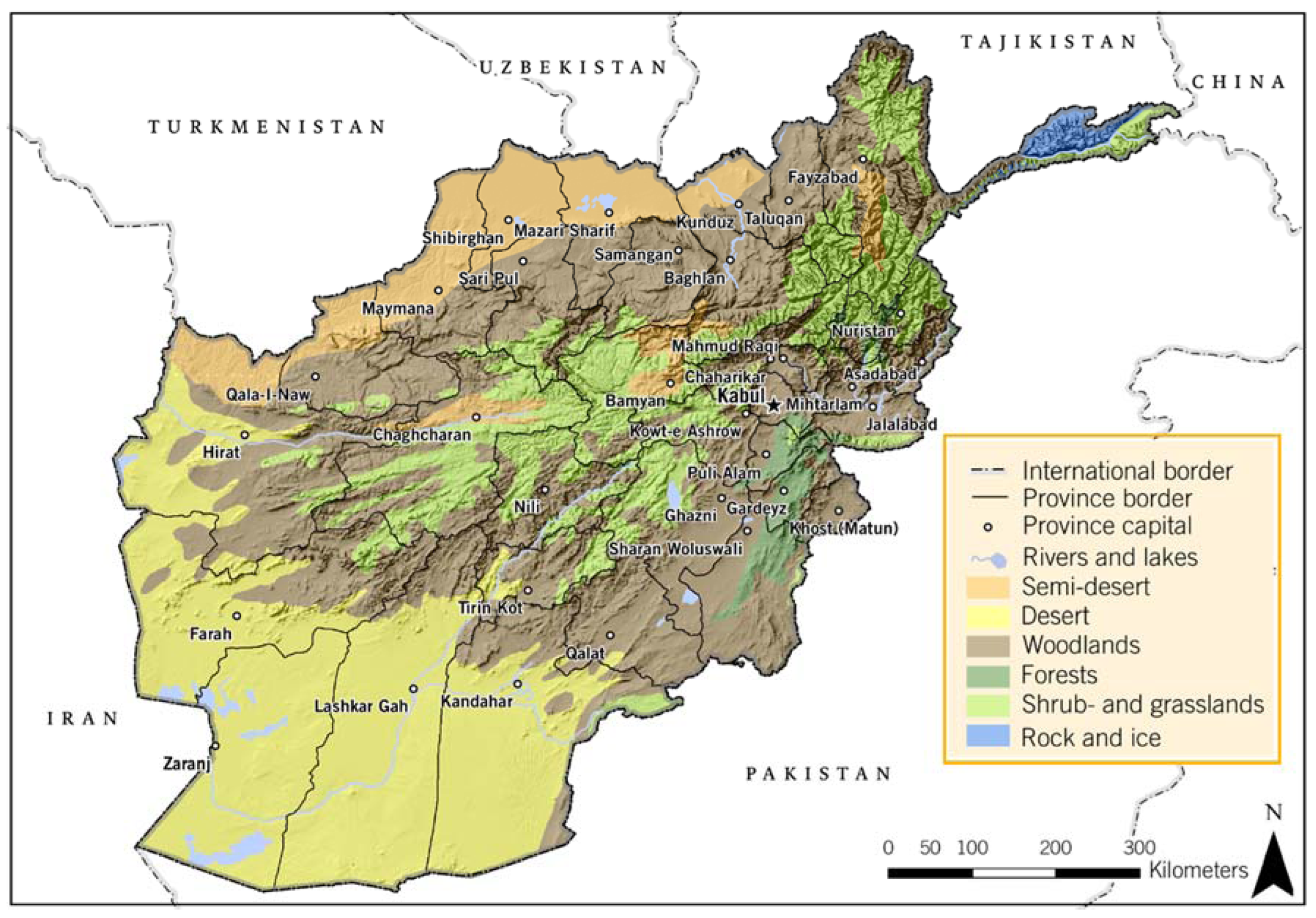
Figure 1. Physical geography of Afghanistan, including major vegetation zones (adapted after [34]) and topography.
Climate 05 00038 g001
Figure 2. Topography (a), climatic regions used in the analysis and available weather stations (b), annual precipitation for the period 1960–1990 [38] (c), and mean annual temperature for the period 1960–1990 [38] (d) in Afghanistan.
Climate 05 00038 g002
Figure 3. Validation of (a) mean monthly temperature and (b) monthly precipitation time series of reanalysis data against observation data for one weather station in each of the six climate regions of Afghanistan and Kabul (Figure 1). Discrepancies are discussed in Section 4.1.
Climate 05 00038 g003
Figure 4. Validation of long-term monthly mean temperature and monthly mean precipitation of reanalysis data against observation data for one weather station in each of the six climate regions of Afghanistan and Kabul (Figure 1) (see Section 2.2.2 for periods). In addition, the spread and the mean of the climate models for the period 1970–1999 are plotted in order to evaluate their performance (see Section 2.2.3 for method). Discrepancies are discussed in Section 4.1.
Climate 05 00038 g004
Figure 5. Maps of differences between the periods 1981–2010 and 1950–1980 based on reanalysis data for (a) mean annual temperature; (b) annual precipitation; (c) Heat Wave Magnitude Index; (d) heavy precipitation; (e) Standardized Precipitation Evapotranspiration Index; (f) spring precipitation; and (g) growing season length. The color scheme is arbitrary but was selected so that predominantly positive changes for livelihood are in green and negative ones in red. Significant changes within a grid cell are marked with a black square (α = 0.05; for method see Section 2.3.2).
Climate 05 00038 g005
Figure 6. Observed changes of seasonality for temperature and precipitation as monthly values for the periods 1951–1980 and 1981–2010 for all Afghanistan and five climate regions derived from reanalysis data.
Climate 05 00038 g006
Figure 7. Difference between maps for projected changes in mean annual temperature, annual precipitation, Heat Wave Magnitude Index (HWMI) and heavy precipitation (95th percentile) for the scenario period 2021–2050 compared to the base period 1975–2005 for the Representative Concentration Pathways (RCPs) 4.5 and 8.5. Please note that unlike in Figure 5, the black points indicate not significance but a measure of uncertainty for the future. The significance can be read for the regions from Table 5. For annual temperature and HWMI all models project an increase for all data points. For annual precipitation and heavy precipitation an agreement of trend direction of >66% of the models is marked with a dot. The color scheme is arbitrary but was selected so that predominantly positive changes for livleihood are green and negative ones red. Please note that projections for annual precipitation for the southern and the central part and for heavy precipitation in general are highly uncertain according to the validation (see Section 4.1).
Climate 05 00038 g007
Figure 8. Temperature projections for Afghanistan until the end of the 21st century for Representative Concentration Pathways 4.5 (green) and 8.5 (red).
Climate 05 00038 g008
Figure 9. Difference in projected changes in Standard Precipitation Evapotranspiration Index (SPEI), spring precipitation (January–April) and growing season length (GSL) for the scenario period 2021–2050 compared to the base period 1975–2005 for the Representative Concentration Pathways 4.5 and 8.5. For SPEI and GSL all models project an increase for all data points. For spring precipitation an agreement of trend direction of >66% of the models is marked with a dot. Please note that projections for spring precipitation for the South and the Centre regions are highly uncertain according to the validation (see Section 4.1).
Climate 05 00038 g009
Figure 10. Projected changes of seasonality for temperature and precipitation as monthly values for the periods 1976–2005 and 2021–2050 for all Afghanistan and five climate regions for Representative Concentration Pathways 4.5 and 8.5.
Climate 05 00038 g010
Table 1. Mean annual temperature and annual precipitation for all of Afghanistan and the defined climate regions (Figure 2b).
Mean Annual Temperature in °CAnnual Precipitation in mm
Afghanistan14.0312
Hindu Kush0.7745
Northern Plains16.2311
Central Highlands5.2332
Eastern Highlands14.7366
Southern Plateau23.3116
Table 2. Periods of available monthly weather data used for the validation of reanalysis and climate model hindcasts.
StationFaizabadMazar-e SharifKabulPanjabHeratGardezKandahar
Period1963–19771958–19781959–19771965–19771958–19881958–19781963–1977
Table 3. Earth system model—regional climate model combinations applied in the study.
General Circulation Models (GCM)/InstituteRegional Climate Models (RCM)/Institute
1.Australian Community Climate and Earth-System Simulator (ACCESS)/Bureau of Meteorology, AustraliaConformal Cubic Atmospheric Model (CCAM) /Commonwealth Scientific and Industrial Research Organisation, Australia
2.Community Climate System Model (CCSM) /National Center for Atmospheric Research in Boulder, USACCAM
3.Centre National de Recherches Météorologiques Climate Model 5.1 (CNRM–CM5)/Centre National de Recherches Météorologiques, FranceRossby Centre regional atmospheric model (RCA4) /Swedish Meteorological and Hydrological Institute, Sweden
4.CNRM–CM5CCAM
5.EC-Earth/Irish Centre for High-End Computing, IrelandRCA4
6.Max-Planck-Institute Earth System Model (MPI-ESM)/Max Planck Institute für Meteorologie, GermanyCCAM
7.MPI-ESMRCA4
8.MPI-ESMRegional Modell (REMO)/Max Planck Institut für Meteorologie, Germany
9.Geophysical Fluid Dynamics Laboratory Climate Model (GFDL−CM)/Geophysical Fluid Dynamics Laboratory, USACCAM
10GFDL-CMRCA4
11.Institut Pierre Simon Laplace Climate Model 5 (IPSL–CM5)/Institut Pierre Simon Laplace, FranceRCA4
12.Model for Interdisciplinary Research on Climate Earth System Model (MIROC−ESM)/Japan Agency for Marine-Earth Science and TechnologyRCA4
13.Norwegian Earth System Model (NorESM) /Bjerknes Centre for Climate Research, NorwayCCAM
Table 4. Trends for mean annual temperature, annual precipitation, Heat Wave Magnitude Index (HWMI) and heavy precipitation (95th percentile) (March–September), Standardized Precipitation Evapotranspiration Index (SPEI), spring precipitation (January–April), and growing season length (GSL) for the period from 1951 to 2010. Significant trends are bold (α = 0.05; for method see Section 2.3.2).
Trends for Mean Annual Temperature in °CTrend for Annual Precipitation in %Trend for HWMITrend for Heavy Precipitation (3–9) in %Trend for SPEITrend for Spring Precipitation (1–4) in %Trend for GSL in Days
Afghanistan1.8−1.01.0−26.9−0.1−6.912.3
Hindu Kush1.05.1−0.13.60.2−3.811.5
North1.6−9.21.1−34−0.4−13.312.5
Centre1.70.50.8−32.5−0.3−5.518.8
East0.66.40.18.50−102.8
South2.4−9.82−17.2−0.1−146.7
Table 5. Projected trends for mean annual temperature, annual precipitation, Heat Wave Magnitude Index (HWMI) and heavy precipitation (95th percentile) (Mar–Sep) for two emission scenarios (RCP 4.5 and 8.5) and for the first half (2006–2050) and the whole 21st century (2006–2099) as model mean and model range. Significant trends (α = 0.05) are marked with an asterisk. Trends where >66% of the models agree in the direction of trend are marked with a “+”. If both criteria apply, the trend is bold (α = 0.05).
RegionPeriodScenarioTrend for Mean Annual Temperature in °CTrend for Annual Precipitation in %Trend for HWMITrend for Heavy Precipitation in %
MeanRangeMeanRangeMeanRangeMeanRange
Afghanistan2006–2050RCP 4.51.71.1–2.9−1.6 +−19.1–24.71.10.4–1.60.4 +−28.4–9.4
RCP 8.52.31.6–3.5−3.8−27.3–18.61.70.7–2.4−2.6 +−29.5–50.9
2006–2099RCP 4.52.72.1–3.6−13.1 *−18.2–332.71–3.9−7.1−32.2–22.1
RCP 8.56.45–8.4−18 *−31.8–22.408.54–14.9−10.5−38.6–34
Hindu Kush2006–2050RCP 4.51.81–3.2−0.1 +−7.6–221.20.1–1.81.9 +−27.5–21.9
RCP 8.52.61.7–3.8−1.3−20.9–9.62.00.7–2.3−4.1−24.1–20.3
2006–2099RCP 4.52.92–4.1−11.3 *−9.7–14.13.41.1–5−2.7 +−20.5–7.5
RCP 8.57.15.3–10.3−14.7 *−25.5–21.4124.4–20.2−12.8 *−35.6–10.3
North2006–2050RCP 4.51.61–2.6−3.1 +−22–47.90.80.1–1.4−2.6−46.6–71
RCP 8.52.31.6–3.5−9.8−26.6–7.21.10.4–1.8−8.5 +−40.4–24.7
2006–2099RCP 4.52.62.1–3.6−16.2 *−20.9–33.51.80.4–2.9−14.6−54.3–16.3
RCP 8.56.24.7–8.2−25−46.8–16.85.82–10.7−20.1 +−72.9–32
Centre2006–2050RCP 4.51.91.1–3−2−25.5–42.81.10.3–1.6−4.4−34.9–19.6
RCP 8.52.41.4–3.6−2.9−30.8–271.80.6–2.58.3 +−26.2–68
2006–2099RCP 4.52.92.2–3.6−14.2 *−26.9–292.91–4−3.5−31.8–29.8
RCP 8.56.75.4–8.7−19.2−37.6–26.88.74–14.4−2.1−51.6–40
East2006–2050RCP 4.51.60.9–2.80.2−28.3–59.31.20.5–1.50.2−12.4–42.5
RCP 8.52.01.1–3.27.1 +−24.2–55.51.50.3–2.33.6+−23.1–56.2
2006–2099RCP 4.52.41–2.8−9.7−14.4–24.82.51.3–3.50.9−25.6–24
RCP 8.55.94.4–7.9−7.3−35.2–42.76.53–12.20.7+−39.8–56.2
South2006–2050RCP 4.51.51.9–3.2−0.1−32.9–37.21.20.5–1.8−0.6−48.4–70.2
RCP 8.52.11.5–3.4−4−51.5–89.61.70.7–2.65.8−75.1–256.8
2006–2099RCP 4.52.41.1–2.9−5.8 +−25.7–41.42.61–42.5 +−50.3–186.1
RCP 8.56.04.5–8.2−13.1 *−44.4–38.48.64.8–15.1−0.4 +−85.5–152.3
Table 6. Future trends for agricultural indices Standardized Precipitation–Evapotranspiration Index (SPEI), spring precipitation (January–April), and growing season length (GSL) for two emission scenarios (RCP 4.5 and 8.5) and for the first half (2006–2050) and the whole 21st century (2006–2099) as model mean and model range. Significant trends (α = 0.05) are marked with an asterisk. Trends where >66% of the models agree in the direction of trend are marked with a “+”. If both criteria apply, the trend is in bold.
RegionPeriodScenarioTrend for SPEITrend for Spring Precipitation in %Trend for GSL in Days
MeanRangeMeanRangeMeanRange
Afghanistan2006–2050RCP 4.5−0.79−1.4–−0.1−3.7−25.5–4916.68.2–27.8
RCP 8.5−0.66−1.2–−0.2−12.9 +−31.6–23.321.59.9–31.8
2006–2099RCP 4.5−1.2−2.1–0.8−15.1 *−25–33.722.418.5–32.2
RCP 8.5−2.32−2.9–−1.5−28.9−58.7–24.35944.6–81.4
Hindu Kush2006–2050RCP 4.5−0.21 +−0.7–0.8−1.9−12.2–3717.21.7–40.8
RCP 8.5−0.08−0.9–0.3−6.3 +−22.4–17.7259.2–54.7
2006–2099RCP 4.5−0.01 +−0.6–1.7−9.3−10.2–32.52015.9–49.4
RCP 8.5−0.44−1.7–0.6−18.9−48.1–32.878.334.5–122.4
North2006–2050RCP 4.5−0.79−1.4–0−3.9−25–30.818.511.1–32.8
RCP 8.5−0.84−1.3–−0.4−16.8−36.1–9.523.46.7–38.9
2006–2099RCP 4.5−1.42−2.3–0−17.4 *−22.4–20.822.920.5–39.2
RCP 8.5−2.64−3.1–−1.8−33.5−66.8–6.464.948.7–91.7
Centre2006–2050RCP 4.5−0.64−1.4–0.3−5.9−38.5–79.719.65.8–35.1
RCP 8.5−0.55−1.2–0.1−13.6−41.7–37.12410.7–37.5
2006–2099RCP 4.5−0.86−1.9–1.3−18.9 *−41.3–44.621.120.8–41.3
RCP 8.5−2.08−3–−0.8−33.4−70.9–25.573.452.7–104.1
East2006–2050RCP 4.5−0.77−1.4–0.1−14.2−42.7–105.919.210.8–26.8
RCP 8.5−0.49−1.4–−0.4−23.8−49.9–56.824.115.7–33
2006–2099RCP 4.5−1.01−2.1–0.4−24.5 *−54.3–45.220.919.4–35.5
RCP 8.5−2.18−2.9–−1.2−39.3−66.1–47.159.844.3–77.9
South2006–2050RCP 4.5−1.28−2–−0.6−7.5−48–172.511.20.9–28.1
RCP 8.5−0.93−1.4–−0.430.2−66.8–60.714.91.1–29.9
2006–2099RCP 4.5−1.99−2.9–0.5−18.5−52.5–46.411.13.4–36.1
RCP 8.5−3.17−3.3–−2.8−44.1−61.4–26.127.959.9–2.6