Ensemble Forecasts: Probabilistic Seasonal Forecasts Based on a Model Ensemble

Abstract

Ensembles of general circulation model (GCM) integrations yield predictions for meteorological conditions in future months. Such predictions have implicit uncertainty resulting from model structure, parameter uncertainty, and fundamental randomness in the physical system. In this work, we build probabilistic models for long-term forecasts that include the GCM ensemble values as inputs but incorporate statistical correction of GCM biases and different treatments of uncertainty. Specifically, we present, and evaluate against observations, several versions of a probabilistic forecast for gridded air temperature 1 month ahead based on ensemble members of the National Centers for Environmental Prediction (NCEP) Climate Forecast System Version 2 (CFSv2). We compare the forecast performance against a baseline climatology based probabilistic forecast, using average information gain as a skill metric. We find that the error in the CFSv2 output is better represented by the climatological variance than by the distribution of ensemble members because the GCM ensemble sometimes suffers from unrealistically little dispersion. Lack of ensemble spread leads a probabilistic forecast whose variance is based on the ensemble dispersion alone to underperform relative to a baseline probabilistic forecast based only on climatology, even when the ensemble mean is corrected for bias. We also show that a combined regression based model that includes climatology, temperature from recent months, trend, and the GCM ensemble mean yields a probabilistic forecast that outperforms approaches using only past observations or GCM outputs. Improvements in predictive skill from the combined probabilistic forecast vary spatially, with larger gains seen in traditionally hard to predict regions such as the Arctic.

1. Introduction

General circulation models (GCMs) that represent atmosphere, ocean and land surface processes can be run to make meteorological predictions weeks to months ahead. Although such long-term or seasonal-scale predictions are not very reliable because uncertainties in initial conditions and in model structure get amplified over time, they are still expected to contain useful information because there are sources of predictability, such as the Southern Oscillation, for this timescale. In recent years, there have been a number of efforts to regularly produce ensembles of GCM seasonal predictions that can inform climate-sensitive applications such as agriculture and water resources. Given the limited GCM skill at these timescales, though, much work remains to be done to convert ensemble predictions into well-calibrated, reliable forecasts [1]. A number of research groups have considered different aspects of using statistical methods to generate such forecasts from GCM ensembles, but many of these methods are more commonly used for and better suited to combining multiple GCMs [2,3,4,5,6,7,8,9]. This paper builds on previous work on the statistical calibration of seasonal predictions of a one GCM ensemble in the case where these projections are expressed as probabilities of each climatology tercile [10].

We extend this previous work to the case where a set of discrete ensemble predictions for the future value of a continuous variable of interest (temperature) are available, along with sets of past observations and predictions (or “postdictions” or “hindcasts”, generated for prior time periods by running a current GCM version initialized using an earlier starting point) made using the same ensemble. We use the sets of previous observations and predictions to construct a reliable forecast, expressed as a probability distribution for the future value of the variable. As in our previous work, we concentrate on three aspects of this task: (a) creating probabilistic forecasts that account for possible biases in the mean and dispersion of the GCM ensemble; (b) quantifying the performance of probabilistic forecasts using information theory metrics, notably the information gain from including the GCM projections in the forecast model compared to either a “climatology” forecast model using only the past observations or a slightly more sophisticated but still simple statistical model based on month-to-month persistence in climate anomalies; (c) studying whether we can better account for the relatively large climate trends of recent decades [11,12], which are not necessarily well represented in the GCMs used for seasonal prediction, through simple statistical methods such as giving more recent observations greater weight than older observations in constructing the climatology and forecast probability distribution.

2. Methods

2.1. Data

We considered monthly mean temperatures on a $1^{\circ }\times 1^{\circ }$ global spatial grid as the meteorological variables to be forecast. For this case study comparing different forecast methods, the observations and GCM postdictions considered cover the period February 1984 to January 2009. The GCM outputs represent 1 month ahead seasonal predictions taken from a hindcast archive for the second version of the NCEP Climate Forecast System (CFSv2), a state-of-the-art operational GCM [13]. The ensemble members were initialized from observations up to various days during the beginning of the month previous to the month whose temperature value was to be forecast; for example, most of the September ensemble members are forecasted in August.

While the CFSv2 has 12 ensemble members, we selected the 9 members $\{g_1,\dots ,g_9\}$ that were present in every month for which the CFSv2 was run. The “observation” temperatures used to calibrate and verify the forecasts were taken from the NCEP CFSv2 reanalysis. Aspects of this hindcast and reanalysis data set have been described and studied elsewhere [14,15,16,17,18,19,20,21].

2.2. Probabilistic Models

We evaluated the skill of the climatology and the forecasts by first assuming that both are normally distributed. We based these models on the average predicted temperature and the spread of the predictions. We used climatology as a baseline by computing the average and spread (μ and σ respectively) of past temperatures. These values were then used to compute a Gaussian pdf of the form:

$$p\left(o\right|t,l)=\frac{1}{\sigma (t,l)\sqrt{2\pi }}\exp \left(\frac{{(o(t,l)-\mu (t,l))}^2}{2\sigma {(t,l)}^2}\right)=\mathcal{N}(\mu ,\sigma )$$

(1)

where $o(t,l)$ is the observation, t is a time index (month and year), l is a spatial index (corresponding to the latitude and longitude of the observation). The μ and σ parameters in the exponential formula for the Gaussian distribution are taken to be space-time dependent. We evaluated the temperature observations, but the methodology is generic to any variable. We explored multiple ways of representing the average and spread, so in some models μ was replaced by the bias-corrected version $\widehat{\mu }$ and σ was replaced by a time averaged Root Mean Square Error . These models p are subscripted by either a c for climatology or an f for forecasts. That letter is further subscripted by a number to indicate that different parameters are used for constructing that model. The simplest model, which is based on the μ and σ for the dataset (climatology or hindcasts) is labeled 0, while other numbers indicate either a different μ or different σ. Throughout the paper, the model is referenced by its letter and number.

2.2.1. A First Probabilistic Forecast Model

For each $1^{\circ }\times 1^{\circ }$ grid point and for each time step (month), we have 9 temperature projections (one for each member of the hindcast ensemble) $\{g_1,\dots ,g_9\}$ from which to produce a forecast distribution. The simplest method to do this is to assume that the hindcasts are normally distributed. Given this naive assumption, the probability density of the hindcast, denoted $h_0$, uses the ensemble mean $\mu (g_1(t,l),\dots ,g_9(t,l))$, at a given forecast time t and location l, for the mean of the forecast normal distribution, and the variance of the hindcasts ${\sigma }^2(g_1(t,l),\dots ,g_9(t,l))$ as its variance:

$$p_{h_0}\left(T\right|t,l)=\mathcal{N}({\mu }_h,{\sigma }_h)$$

(2)

In order to understand whether or not this is a good probabilistic forecast model, we must first establish an evaluation metric.

2.2.2. Information Gain Over Climatology

Climatology itself can be considered a reasonably effective baseline predictor of monthly mean temperatures because the monthly temperature field does not vary much between years; for example, while the global mean temperature for January is 276 K, the mean inter-annual standard deviation of grid-cell January temperatures averages only 1.5 K. For our baseline climatology model, we take a normal distribution based on the running mean ${\mu }_c$ and running standard deviation ${\sigma }_c$ of the observations. Although the running statistics suffer from high sampling variability, they are used so that our analysis models real world conditions wherein data is only available as it comes, meaning that January 2008 has no awareness of March 2008. The running statistics are computed as the mean and standard deviation, respectively, of all observations $t^{\prime }$ occurring in the same month as t for all years prior to t:

$${\mu }_c(t,l)={\langle o(t^{\prime },l)\rangle }_{t^{\prime }\in M_t}$$

(3)

$${\sigma }_c(t,l)={\langle {(o(t^{\prime },l)-{\mu }_c(t^{\prime },l))}^2\rangle }_{t^{\prime }\in M_t}^{\frac{1}{2}}$$

(4)

where $M_t=\left\{t^{\prime }\right|t^{\prime }<t,\mathrm{month}\left(t^{\prime }\right)=\mathrm{month}\left(t\right)\}$. This is then used to compute the probability distribution:

$$p_{c_0}\left(T\right|t,l)=\mathcal{N}({\mu }_c,{\sigma }_c)$$

(5)

While probability density functions (distributions) may be compared by many metrics, a natural measure for the ability to represent observed values is information gain, which is also known as the Kullback-Leibler divergence [22,23,24]. The Kullback-Leibler divergence was chosen because it can be decomposed into three diagnostically useful components: (1) reliability: conditional bias in the forecast relative to observations; (2) resolution: the forecast’s skill in explaining the observational uncertainty; (3) uncertainty: the initial uncertainty in the observation [25]. Information gain was chosen over the computationally similar ignorance score IGN (itself just the mathematical inverse of IG) because IG is a more robust measure of the same quantity [23,26,27].

To compute the information gain, we first compute the negative log likelihood of the probability of the observed measurement occurring in the distribution constructed from climatology ($c_0$):

$$NLL\left(c_0\right)=-{\log }_2\left(p_{c_0}\left(o\right|t,l)\right)$$

(6)

The negative log likelihood described by Equation (6) is also interpreted as a measure of how surprising the observation is with respect to our probabilistic prediction p. We subtract the negative log likelihood of the model being evaluated from the negative log likelihood of the baseline model to measure the information gain:

$$IG(model,c_0)=\langle NLL\left(c_0\right)-NLL\left(model\right)\rangle$$

(7)

We chose the climatology distribution $c_0$ as our baseline because it is based solely on observational measurements and so it does not rely on the GCM output. We then evaluated all the other probabilistic models against this baseline by averaging the IG temporally and spatially. A skilled forecast will have, on average, lower NLL than the baseline forecast because it should be less surprised by the observation than climatology, yielding a net positive IG. To ascertain whether the differences in mean IG seen between probabilistic methods are robust to the choice of time interval over which they were tested, we evaluate the significance of differences in mean IG between methods using Student’s t-test on the monthly time series of the difference in mean IG between two methods, with the degrees of freedom adjusted based on the observed lag-1 autocorrelation of the time series [28]. We found that differences of 0.01 bit or more in mean IG were generally significant at the 95% confidence level.

Figure 1 illustrates how the probabilistic models are created and evaluated. The probability density $p_{h_0}$ is constructed using Equation (2) from the mean and standard deviation of the CSFV2 hindcast predicted values $g_i$ at t,l, which are shown under $p_{h_0}$ as dots. The baseline climatology distribution $p_{c_0}$ is constructed from the mean and standard deviation of the historical observations $o{(t^{\prime },l)}_{t^{\prime }\in M_t}$ using Equation (5). The straight line that cuts across the figure is the observed (true) temperature at time t, location l, which in this example is quite far from the mean of the hindcast values $g_i$. Although this example is specific to November 2004 in the equatorial Atlantic ocean, this behavior is typical; with respect to IG, the naive probabilistic forecast method of Equation (2) is not particularly accurate when compared to climatology.

2.3. Improved Probabilistic Models

In the section that follows, we sought to increased the quantifiable skill of the model by accounting for biased predictions and better incorporating the variability of the observed measures.

2.3.1. Bias-Corrected Probabilistic Model

In order to improve the probabilistic forecast presented in Equation (2), we can take into account one well known source of error, GCM prediction bias [17,20,29,30]. In order to remove the bias, we subtract the mean GCM error for the same calendar month over previous years (for the same grid point l) with respect to the observation:

$${\widehat{\mu }}_h(t,l)={\mu }_h(t,l)-{\langle {\mu }_h(t^{\prime },l)-o(t^{\prime },l)\rangle }_{t^{\prime }\in M_t}$$

(8)

We replaced ${\mu }_h$ with ${\widehat{\mu }}_h(t,l)$ to obtain a new probabilistic formula:

$$p_{h_1}\left(o\right|t,l)=\mathcal{N}(\widehat{{\mu }_h},{\sigma }_h)$$

(9)

While this improved the IG of the probabilistic forecast, there was a spatial pattern of large negative IG in the Antarctic region.

As seen in Figure 2, this localized behavior is largely due to a small ensemble spread but relatively large spread in the actual observations in certain regions of the maps. The poor model performance indicates that the uncertainty of the forecast is not well captured by the spread in the individual ensemble projections and may be better captured by a different measure such as the climatology spread or forecast RMSE.

2.3.2. Climatological Variance Adjusted Probabilistic Models

Figure 2 illustrates that forecast is sometimes a poor proxy for spread due to overconfidence in highly variable regions. This is also shown in Figure 1, where the bias-corrected forecast $p_{h_1}$ has a narrower range of potential temperatures than historical observations have recorded for that location. This motivated us to explore the use of climatology spread ${\sigma }_c$ as a proxy for error. The probabilistic model $h_2$ is computed as:

$$p_{h_2}\left(o\right|t,l)=\mathcal{N}({\widehat{\mu }}_h,{\sigma }_c)$$

(10)

where the climatology standard deviation replaces the use of the spread of the GCM ensemble as the standard deviation σ in the normal distribution of the probabilistic forecast. In Figure 1, the probability of the measured temperature (black line) computed using the $h_2$, $h_0$ and $c_0$ models. Model $h_2$ reports the highest likelihood of the temperature occurring, as illustrated by $p_{h_2}\left(o\right|t,l)$ (pink dot) being of greater value than $p_{c_0}\left(o\right|t,l)$ (cyan dot). By removing the bias and replacing the ensemble uncertainty ${\sigma }_f$ with the climatology standard deviation ${\sigma }_c$, we obtained a probabilistic forecast which usually outperforms the climatology forecast (positive IG).

2.3.3. Mean Adjusted Forecast RMSE Adjusted Probabilistic Models

Since Figure 2d indicated that the mean adjusted forecast ${\widehat{\mu }}_h$ RMSE is similar to the overall climatology spread, we constructed a model that used the time averaged RMSE as a proxy for uncertainty. We computed the time averaged RMSE as:

$${RMSE}_{{\widehat{\mu }}_h}(t,l)=\sqrt{{\langle {({\widehat{\mu }}_h(t^{\prime },l)-o(t^{\prime },l))}^2\rangle }_{t^{\prime }\in M_t}}$$

(11)

Using this time-averaged RMSE, the probabilistic model $h_3$ is computed as:

$$p_{h_3}\left(o\right|t,l)=\mathcal{N}({\widehat{\mu }}_h,{RMSE}_{{\widehat{\mu }}_h})$$

(12)

where the time averaged root mean squared error is now the standard deviation σ in the normal distribution of the probabilistic forecast. As a time averaged RMSE it is very sensitive in the early parts of the time series, but improves significantly over time.

2.4. Autoregressive Models

The improvement in forecast skill through the incorporation of information from climatology, as described in Section 2.3.1, motivated us to explore the contributions of some of the many input variables the CFSv2 uses to generate a prediction for a point. We were particularly interested in the historical values of physical variables at the grid point l because climatology is derived from those variables. One way to clarify the relevance of this information is to build a simple statistical forecast model, progressively incorporating more of the past observations. Besides giving us a new benchmark against which we can judge the added value of running CFSv2 or similar GCMs for long term forecasting, such statistical models can also give us some indications of which variables are most informative for the future state of the climate system.

We name these statistical forecast models as R (for regression) and use positional subscripts to denote the parameters on which the model is fit. The first subscript c or h indicates the absence or inclusion, respectively, of hindcasts. The second and third subscripts indicate the presence w or absence e of weighting in computing the climatology and regression respectively. This weighting scheme is discussed in Section 2.4.3. These statistical forecast models also yield predictions q, notated as $cr$ when hindcasts are omitted and $hr$ when they are included. We include an r in the error notation to distinguish the statistical computations used for the regression models from the ones discussed in Section 2.2.

2.4.1. Autoregressive Climatology

We consider a very simple linear auto-regressive model which uses data from two and three months prior. We do not use the preceding month’s data because it would not be available for use in a forecast until the end of the month being predicted, but we include prior data so that we can incorporate seasonal trends to some degree. The model first fits a forecast based on a linear combination of the climatology mean and the observations two months and three months prior to the observation being predicted.

$$q_{cr}(t,l)=\alpha (t,l){\mu }_c(t,l)+{\beta }_1(t,l)o(t-2,l)+{\beta }_2(t,l)o(t-3,l)$$

(13)

where α, ${\beta }_1$, and ${\beta }_2$ are the weights computed using a linear regression that employs observations from previous time-steps $t^{\prime }\in M_t$. We then bias correct the predictions by subtracting the running bias:

$${\widehat{q}}_{cr}(t,l)=q_{cr}(t,l)-{\langle q_{cr}(t^{\prime },l)-o(t^{\prime },l)\rangle }_{t^{\prime }\in M_t}$$

(14)

In order to build a probabilistic forecast, we need to estimate its uncertainty, so at a given time t and location l the time averaged distribution of errors is computed as:

$${RMSE}_{{\widehat{q}}_{cr}}(t,l)=\sqrt{{\langle {({\widehat{q}}_{cr}(t^{\prime },l)-o(t^{\prime },l))}^2\rangle }_{t^{\prime }\in M_t}}$$

(15)

The RMSE represents the historical error and thus is a good proxy for the uncertainty in the forecast. We then use the bias-corrected prediction and the RMSE to construct the probabilistic forecast:

$$R_{cee}=p_{cr}\left(T\right|t,l)=\mathcal{N}({\widehat{q}}_{c}r,{RMSE}_{{\widehat{q}}_{c}r})$$

(16)

2.4.2. Combined GCM-Autoregressive Forecast Model

In Section 2.3 we saw that removal of the hindcast bias and replacement of the standard deviation with climatological uncertainty (standard deviation) in the normal distribution results in an improvement of the GCM ensemble based probabilistic forecast. Because combining the hindcasts and climatology yielded a better forecast, we fit a linear combination of the bias-corrected mean hindcasts, the climatology, the 2-month lookback, and the 3-month lookback to test if that will further improve the forecast. Defining γ as the weight of the hindcasts’ contribution to the model, we compute a combined GCM-autoregression forecast with mean:

$$q_{hr}(t,l)=\alpha (t,l){\mu }_c(t,l)+{\beta }_1(t,l)o(t-2,l)+{\beta }_2(t,l)o(t-3,l)+\gamma (t,l){\widehat{\mu }}_h(t,l)$$

(17)

This fitting should at least not greatly worsen performance of the forecast compared to the probabilistic model $h_2$ described in Section 2.4.1. When the distribution is normal, the IG is essentially the squared error in the forecast mean; therefore fitting predictor coefficients by least squares should reduce the error. The combined model performance should also be at least comparable to that of the probabilistic model because $h_2$ is a special case of the regression in which the coefficients are $\alpha ={\beta }_1={\beta }_2=0$ and $\gamma =1$.

As with the model in Section 2.4.1, we bias correct $q_{hr}$:

$${\widehat{q}}_{hr}(t,l)=q_{hr}(t,l)-{\langle q_{hr}(t^{\prime },l)-o(t^{\prime },l)\rangle }_{t^{\prime }\in M_t}$$

(18)

and then take the uncertainty to be the time averaged root mean square error:

$${RMSE}_{{\widehat{q}}_{hr}}(t,l)=\sqrt{{\langle {({\widehat{q}}_{hr}(t^{\prime },l)-o(t^{\prime },l))}^2\rangle }_{t^{\prime }\in M_t}}$$

(19)

The combined climatology and forecast model is therefore:

$$R_{hee}=p_{hr}\left(T\right|t,l)=\mathcal{N}({\widehat{q}}_{hr},{RMSE}_{{\widehat{q}}_{hr}})$$

(20)

We considered fitting a regression model for an initial portion of the data, e.g., the first 1/3, and applying it to the remainder of the time series, but this gave poor results. There are indications that this is because slowly changing means progressively make the autoregressive statistical forecast worse. The model was therefore modified so that the coefficients would be updated on every new observation, making it an online algorithm ($R_{cee}$ and $R_{hee}$).

2.4.3. Auto-Regressive Weights

We considered further modifying the auto-regressive forecast model to better account for climatology trends. To accomplish this, climatology computed using the running average was replaced with climatology computed using an exponentially weighted moving average (EWMA) that more heavily weights recent observations. Weights are applied to the observations as follows:

$${(1-\lambda )}^{n-1},{(1-\lambda )}^{n-2},\dots ,1-\lambda ,1$$

(21)

wherein 1 is the weight of the most recent observation and λ is:

$$\lambda =2/(s+1)$$

(22)

where s is the span of the EWMA. We investigated three methods of incorporating EWMA weighting:

• computing the climatology using EWMA ($R_{cwe}$, $R_{hwe}$)
• updating the weights in the online regression using EWMA ($R_{cew}$, $R_{hew}$)
• combining methods 1 and 2 ($R_{cww}$, $R_{hww}$)

We used a span s of 17 years for EWMA analyses because it gave the highest mean information gain of all the spans we tested, which ranged from 1 to 30 years in increments of 1 year. This is very similar to the optimum EWMA span found in an analysis of station monthly temperature data [12].

3. Results

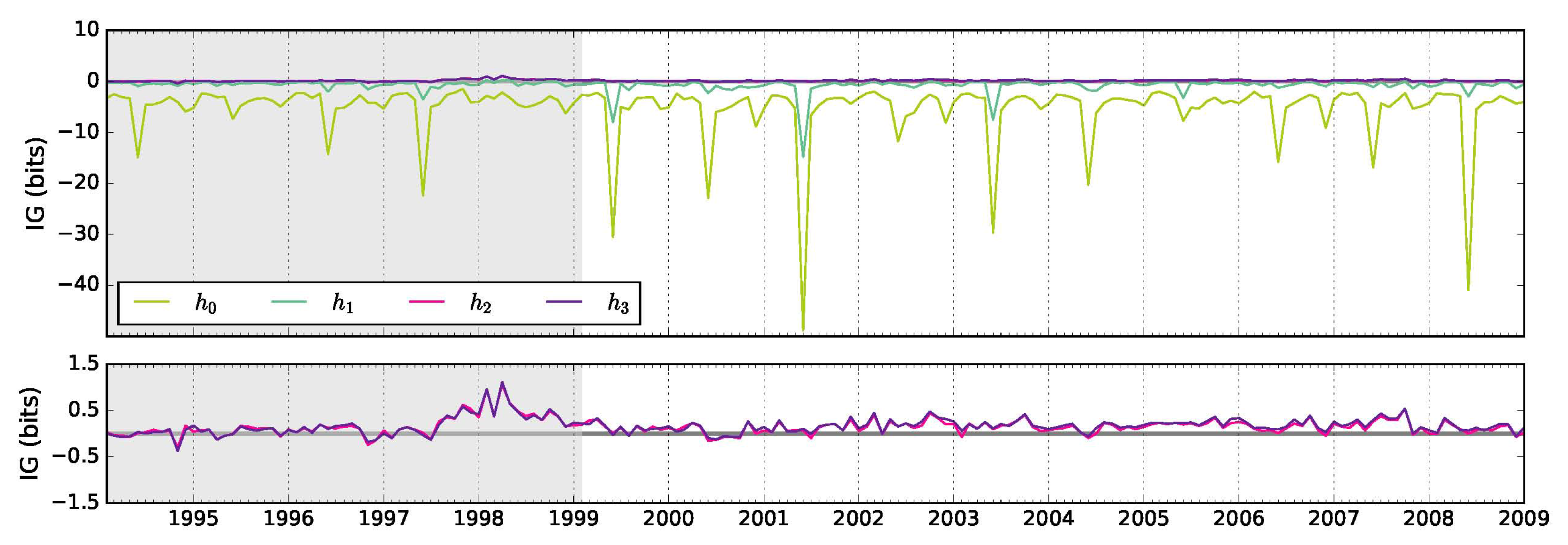
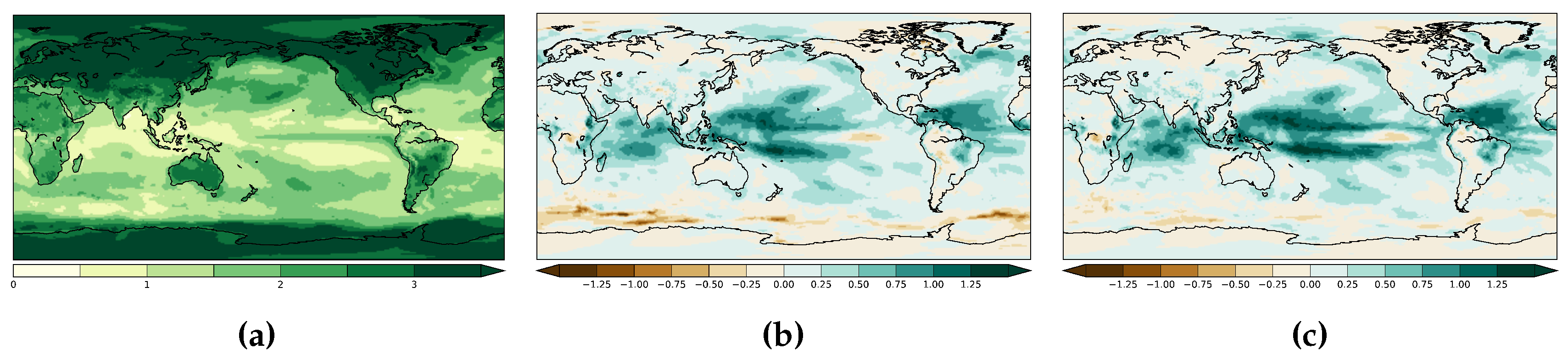
3.1. Non-Auto-Regressive Probabilistic Models

Information gain is the difference in the negative log likelihood (NLL), as shown in Equation (7). NLL measures the probability of an observation occurring in a distribution, with lower NLL indicating a better probabilistic model. $c_0$ was used as the baseline model for all the comparisons. In Figure 3 and

Table 1. Gaussian probabilistic models were constructed using the listed parameters for the mean and standard deviation. The IG of the model is computed relative to the baseline model $c_0$ and the table reports the IG averaged over space and time between 1999 and 2009. $h_2$ and $h_3$ are the most skilled models because they have largest positive mean. Models are statistically distinguishable from each other if they differ by at least 0.01 bit at an α level of 0.05 .

IG of $\mathcal{N}(\mathbf{\mu },\mathbf{\sigma })$ Relative to ${\mathit{c}}_{\mathbf{0}}$
Model	Param.		Mean	Median
$c_0$	${\mu }_c$	${\sigma }_c$	- - - -	- - - -
$h_0$	${\mu }_h$	${\sigma }_h$	–5.602	–0.410
$h_1$	${\widehat{\mu }}_h$	${\sigma }_h$	–0.858	0.151
$h_2$	${\widehat{\mu }}_h$	${\sigma }_c$	0.140	0.035
$h_3$	${\widehat{\mu }}_h$	${RMSE}_{{\widehat{\mu }}_h}$	0.169	0.037

the models that use ensemble spread as a measure of uncertainty, $h_0$ and $h_1$ are highly susceptible to seasonal regularly recurring overconfidence. Together with the spatial maps of uncertainty shown in Figure 2 we can pinpoint the errors as occurring in the poles in May. The lower graph in Figure 3 removes the models based on ${\sigma }_f$ to more clearly illustrate the improvements in IG gained through using better proxies for error. These two models, $h_2$ and $h_3$ , are for the most part statistically indistinguishable from each other, a similarity which can be seen in how close their time series are to each other in Figure 3. Both models show improvement over time, yielding mostly positive IG in the latter part of the timeseries.

Figure 3 shows that the forecasting skill of the $h_2$ model improves over time. This may be because the standard deviation may more accurately capture the forecast uncertainty as more historic data points are added into the computation. Model $h_2$ yielded some gains in the tropical Pacific, which are shown in Figure 4b, but overall it did not do well in many of the same regions in which $c_0$ is also unskilled. This is indicated by the high RE in Figure 4a across North America, Asia, and Antarctica. The limited IG gains achieved by using a model based on GCM predictions further motivated the development of regression models that, as described in Section 2.4.2, combine both historical data and the GCM predictions.

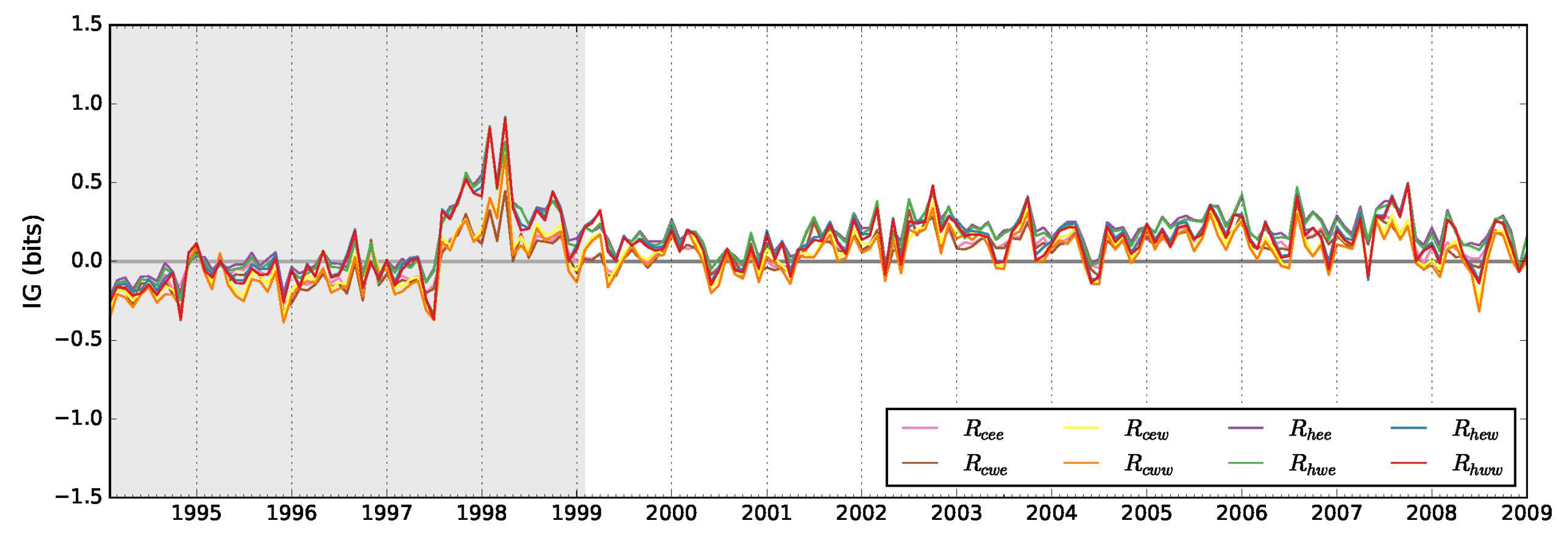
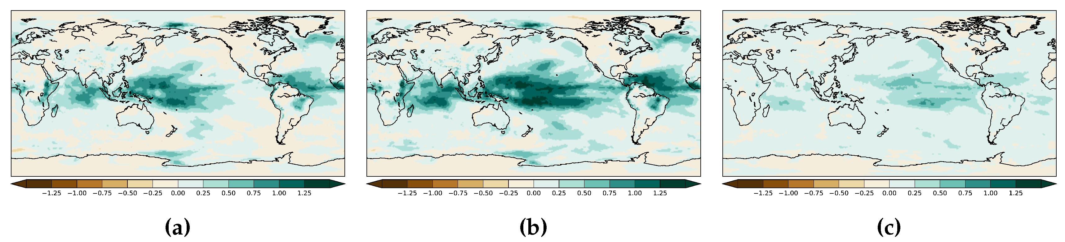
3.2. Auto-Regressive Models

The various auto-regression based models are very unskilled at the beginning of the time series, as shown in Figure 5, because they overfit the little data they have. However, for the entire evaluation period,

Table 2. Gaussian probabilistic models were constructed using the regression’s predicted value q as the mean. ${\sigma }_{cr}$ or ${\sigma }_{fr}$, for climatology only and forecast inclusive regressions, were used as the standard deviation. The IG of the model is computed relative to the baseline model $c_0$ and the table reports the IG averaged over space and time between 1999 and 2009. While $R_{hee}$ is the most skilled based on mean and median IG, the scores between the various forecast inclusive models are very similar. Models are statistically distinguishable from each other if the differ by at least 0.01 bit at an α level of 0.05.

IG $\mathcal{N}(\widehat{\mathit{q}},RMSE)$ Relative to ${\mathit{c}}_{\mathbf{0}}$
Model	Hindcasts	EWMA Weighted		Mean	Median
		Climatology	Regression
$R_{cee}$	no	no	no	0.112	–0.053
$R_{cwe}$	no	yes	no	0.095	–0.084
$R_{cew}$	no	no	yes	0.095	–0.056
$R_{cww}$	no	yes	yes	0.067	–0.074
$R_{hee}$	yes	no	no	0.200	0.005
$R_{hwe}$	yes	yes	no	0.190	–0.011
$R_{hew}$	yes	no	yes	0.151	–0.014
$R_{hww}$	yes	yes	yes	0.137	–0.0033

reports that all the methods perform better than $c_0$.

Figure 6a,b show that the auto-regressive models also yield improved skill in some of the regions that climatology does poorly in, specifically North America and Central Asia. Figure 6c shows very strong skill in the tropical Pacific, like all the forecast models, and that that skill has spread to much of the equatorial landmass. The predictions in the Arctic and Antarctic are also not as unskilled as in the other models.

Figure 7 shows the coefficients of the forecast auto-regression. While the climatology coefficient appears to contribute the most to the regression, GCM predictions are not very far behind. There also appears to be a trade off wherein the GCM prediction coefficient contributes strongly to regions, such as the tropical Pacific, weakly contributed to by climatology. The 2-month and 3-month lookback coefficients (${\beta }_1$ and ${\beta }_2$ respectively) contribute almost negligibly to the regression, except for a slight peak in the tropical Pacific for ${\beta }_1$. Figure 7 indicates that the coefficients remain fairly consistent along the entire later portion of the time series.

4. Discussion

We have introduced and evaluated several probabilistic models for combining GCM ensemble predictions with climatology and autoregression to produce long term meteorological forecasts. We have shown that a probabilistic model based on GCM predictions alone, even when they are corrected for bias, does not outperform a baseline probabilistic model based only on climatology because the GCM ensemble sometimes suffers from unrealistically little dispersion. However, when we integrated the bias-corrected predictions with the standard deviation of the climatology, we obtained a modified probabilistic forecast model which outperformed the baseline. We then examined a set of models which incorporated an autoregressive 2-month and 3-month lookback. When used as a pure statistical model, it is not as effective as a model that incorporates GCM predictions but is more skilled at predicting observations than the plain climatology model. When we combined the GCM projections with the autoregression, we obtained a combined model which is superior to all models considered in the global average. It appears to produce the most improvement near the Equator, at the expense of slightly poorer performance near the poles. We investigated weighting schemes to incorporate trends, but found that they yielded only small further improvement, possibly because of the relatively short time series of observations used. We found that the contribution of the 3-month lookback was quite weak and that further lookback terms do not contribute. We did not consider spatial statistical correlations, but conjecture that they may contribute to a further improved forecast model. Also, note that the GCM ensemble members used here are all from a single GCM (with different initial conditions) and were therefore treated as interchangeable. Multimodel GCM ensembles, such as the North American Multi-Model Ensemble (NMME) [31] facilitate the exploration of incorporating traditional multimodel calibration methods, such as EMOS and BMA [5,6], into the tools introduced here [32]. Multimodel GCMs also offer the additional possibility of investigating differentially weighting projections from different GCMs based on their demonstrated skill through further extensions of these tools.

References

1. National Research Council. Assessment of Intraseasonal to Interannual Climate Prediction and Predictability; National Research Council: Washington, DC USA, 2010. [Google Scholar]
2. Krishnamurti, T.N.; Kishtawal, C.M.; LaRow, T.E.; Bachiochi, D.R.; Zhang, Z.; Williford, C.E.; Gadgil, S.; Surendran, S. Improved weather and seasonal climate forecasts from multimodel superensemble. Science 1999, 285, 1548–1550. [Google Scholar] [CrossRef] [PubMed]
3. Palmer, T.N. Predicting uncertainty in forecasts of weather and climate. Rep. Prog. Phys. 2000, 63, 71–116. [Google Scholar] [CrossRef]
4. Barnston, A.G.; Mason, S.J.; Goddard, L.; Dewitt, D.G.; Zebiak, S.E. Multimodel ensembling in seasonal climate forecasting at IRI. Bull. Am. Meteorol. Soc. 2003, 84, 1783–1796. [Google Scholar] [CrossRef]
5. Gneiting, T.; Raftery, A.E.; Westveld, A.H.; Goldman, T. Calibrated probabilistic forecasting using ensemble model output statistics and minimum CRPS estimation. Mon. Weather Rev. 2005, 133, 1098–1118. [Google Scholar] [CrossRef]
6. Raftery, A.E.; Gneiting, T.; Balabdaoui, F.; Polakowski, M. Using Bayesian model averaging to calibrate forecast ensembles. Mon. Weather Rev. 2005, 133, 1155–1174. [Google Scholar] [CrossRef]
7. Johnson, C.; Swinbank, R. Medium-range multimodel ensemble combination and calibration. Q. J. R. Meteorol. Soc. 2009, 135, 777–794. [Google Scholar] [CrossRef]
8. Weigel, A.P.; Liniger, M.A.; Appenzeller, C. Seasonal ensemble forecasts: Are recalibrated single models better than multimodels? Mon. Weather Rev. 2009, 137, 1460–1479. [Google Scholar] [CrossRef]
9. Bundel, A.; Kryzhov, V.; Min, Y.M.; Khan, V.; Vilfand, R.; Tishchenko, V. Assessment of probability multimodel seasonal forecast based on the APCC model data. Russ. Meteorol. Hydrol. 2011, 36, 145–154. [Google Scholar] [CrossRef]
10. Krakauer, N.Y.; Grossberg, M.D.; Gladkova, I.; Aizenman, H. Information content of seasonal forecasts in a changing climate. Adv. Meteorol. 2013, 2013, 480210. [Google Scholar] [CrossRef]
11. Krakauer, N.Y.; Fekete, B.M. Are climate model simulations useful for forecasting precipitation trends? Hindcast and synthetic-data experiments. Environ. Res. Lett. 2014, 9, 024009. [Google Scholar] [CrossRef]
12. Krakauer, N.Y.; Devineni, N. Up-to-date probabilistic temperature climatologies. Environ. Res. Lett. 2015, 10, 024014. [Google Scholar] [CrossRef]
13. Saha, S.; Moorthi, S.; Wu, X.; Wang, J.; Nadiga, S.; Tripp, P.; Behringer, D.; Hou, Y.T.; ya Chuang, H.; Iredell, M.; et al. The NCEP climate forecast System Version 2. J. Clim. 2014, 27, 2185–2208. [Google Scholar] [CrossRef]
14. Yuan, X.; Wood, E.F.; Luo, L.; Pan, M. A first look at Climate Forecast System version 2 (CFSv2) for hydrological seasonal prediction. Geophys. Res. Lett. 2011, 38, L13402. [Google Scholar] [CrossRef]
15. Kumar, A.; Chen, M.; Zhang, L.; Wang, W.; Xue, Y.; Wen, C.; Marx, L.; Huang, B. An analysis of the nonstationarity in the bias of sea surface temperature forecasts for the NCEP Climate Forecast System (CFS) Version 2. Mon. Weather Rev. 2012, 140, 3003–3016. [Google Scholar] [CrossRef]
16. Zhang, Q.; van den Dool, H. Relative merit of model improvement versus availability of retrospective forecasts: the case of Climate Forecast System MJO prediction. Weather Forecast. 2012, 27, 1045–1051. [Google Scholar] [CrossRef]
17. Barnston, A.G.; Tippett, M.K. Predictions of Nino3.4 SST in CFSv1 and CFSv2: a diagnostic comparison. Clim. Dyn. 2013, 41, 1615–1633. [Google Scholar] [CrossRef]
18. Luo, L.; Tang, W.; Lin, Z.; Wood, E.F. Evaluation of summer temperature and precipitation predictions from NCEP CFSv2 retrospective forecast over China. Clim. Dyn. 2013, 41, 2213–2230. [Google Scholar] [CrossRef]
19. Kumar, S.; Dirmeyer, P.A.; Kinter, J.L., III. Usefulness of ensemble forecasts from NCEP Climate Forecast System in sub-seasonal to intra-annual forecasting. Geophys. Res. Lett. 2014, 41, 3586–3593. [Google Scholar] [CrossRef]
20. Narapusetty, B.; Stan, C.; Kumar, A. Bias correction methods for decadal sea-surface temperature forecasts. Tellus 2014, 66A, 23681. [Google Scholar] [CrossRef]
21. Silva, G.A.M.; Dutra, L.M.M.; da Rocha, R.P.; Ambrizzi, T.; Érico, L. Preliminary analysis on the global features of the NCEP CFSv2 seasonal hindcasts. Adv. Meteorol. 2014, 2014, 695067. [Google Scholar] [CrossRef]
22. Weijs, S.V.; Schoups, G.; van de Giesen, N. Why hydrological predictions should be evaluated using information theory. Hydrol. Earth Syst. Sci. 2010, 14, 2545–2558. [Google Scholar] [CrossRef]
23. Peirolo, R. Information gain as a score for probabilistic forecasts. Meteorol. Appl. 2011, 18, 9–17. [Google Scholar] [CrossRef]
24. Tödter, J. New Aspects of Information Theory in Probabilistic Forecast Verification. Master’s Thesis, Goethe University, Frankfurt, Germany, 2011. [Google Scholar]
25. Weijs, S.V.; van Nooijen, R.; van de Giesen, N. Kullback–Leibler divergence as a forecast skill score with classic reliability–resolution–uncertainty decomposition. Mon. Weather Rev. 2010, 138, 3387–3399. [Google Scholar] [CrossRef]
26. Jolliffe, I.T.; Stephenson, D.B. Proper scores for probability forecasts can never be equitable. Mon. Weather Rev. 2008, 136, 1505–1510. [Google Scholar] [CrossRef]
27. Jolliffe, I.T.; Stephenson, D.B. Forecast Verification; John Wiley & Sons, Ltd.: Hoboken, NJ, USA, 2011. [Google Scholar]
28. Krakauer, N.Y.; Puma, M.J.; Cook, B.I. Impacts of soil-aquifer heat and water fluxes on simulated global climate. Hydrol. Earth Syst. Sci. 2013, 17, 1963–1974. [Google Scholar] [CrossRef]
29. Cui, B.; Toth, Z.; Zhu, Y.; Hou, D. Bias correction for global ensemble forecast. Weather Forecast. 2012, 27, 396–410. [Google Scholar] [CrossRef]
30. Williams, R.M.; Ferro, C.A.T.; Kwasniok, F. A comparison of ensemble post-processing methods for extreme events. Q. J. R. Meteorol. Soc. 2013. [Google Scholar] [CrossRef]
31. Kirtman, B.P.; Min, D.; Infanti, J.M.; Kinter, J.L.; Paolino, D.A.; Zhang, Q.; van den Dool, H.; Saha, S.; Mendez, M.P.; Becker, E.; et al. The North American Multi-Model Ensemble (NMME): Phase-1 seasonal to interannual prediction, Phase-2 toward developing intra-seasonal prediction. Bull. Am. Meteorol. Soc. 2014, 95, 585–601. [Google Scholar] [CrossRef]
32. Aizenman, H.; Grossberg, M.; Gladkova, I.; Krakauer, N. Longterm Forecast Ensemble Evaluation Toolkit. Available online: https://bitbucket.org/story645/libltf (accessed on 28 March 2016).
Figure 1. Estimating the skill of models predicting the temperature for November 2004 at a grid point on the equatorial Atlantic ocean (12 S, 356 E). The probability density p h 0 is a naive normal (Gaussian) distribution constructed using the 9 CFSv2 hindcasts { g 1 , , g 9 } at a single point l for the date t; the bias-corrected (mean shifted) version is p h 1 . The historical observations o ( t , l ) t M t , restricted to the same calendar month as t, at l are used to construct p c 0 . The bias-corrected mean of the forecasts and the standard deviation of the climatology is used to build p h 2 . The information gain is the difference between p h 2 ( o | t , l ) and p c 0 ( o | t , l ) .
Climate 04 00019 g001
Figure 2. The deviation in the predicted ensembles is consistently lower than what is shown in both the climatology σ c and the error RMSE μ ^ h , as seen in the temporal averages shown in (bd) and the spatial average over the non-shaded time period in (a). The ensemble spreads tendency towards lower uncertainty is especially evident in the polar regions, which indicates overconfidence in the predictions for those regions; this over-confidence persists even after the forecast has been bias-corrected, as in (d). The shaded period is shown for consistency with the other graphs but is omitted from later calculations.
Climate 04 00019 g002
Figure 3. The predictive skill of c 0 is used as the baseline against which all the other models are compared because it is based solely on past observations. The spikes in IG only occur in the models that use σ f , h 0 and h 1 so these models are removed in the lower graph to highlight that the models based on other proxies for uncertainty, h 2 and h 3 are not susceptible to these errors and show positive information gain in the later part of the time series. The shaded portion of the time series is omitted from later analysis but is shown here to demonstrate that the IG grows more positive over time.
Climate 04 00019 g003
Figure 4. These maps are the averages of NLL and IG for each grid point from February 1999 to January 2009. Climatology can be used to build a fairly good predictor in the tropical oceans, but falters on most landmasses as shown by the higher NLL in (a). The models h 2 and h 3 which incorporate the hindcasts and the climatology mostly do better in regions such as the ocean where c 0 already does well, but they also show small gains on land, especially in the northern hemisphere. As seen in (b,c), h 3 does slightly better in the ENSO region but otherwise h 3 and h 2 are mostly indistinguishable.
Climate 04 00019 g004
Figure 5. While all the regression based probabilistic forecast models ( R c e e R c w e R c e w R c w w R h e e R h w e R h e w R h w w ) have very similar skill, the combined models ( R h e e R h w e R h e w R h w w ) are consistently more skilled, especially as the data becomes positive. Each time series is the spatial average of the global NLL at each observation time. The shaded region is not used in further analysis.
Climate 04 00019 g005
Figure 6. The auto-regressive model yields small improvements on land over the simpler model shown in Figure 4. Figure 6c shows that R h e e is generally more skilled than R c e e over land, especially in the ENSO region. While there is a lack of skill in the Arctic and Antarctic, the difference is very small. As with Figure 4, these maps are the temporal average between 1999 and 2009 as that is the period when the IG improves. (a) μ ( IG ( R c e e , c 0 ) ) . (b) μ ( IG ( R h e e , c 0 ) ) . (c) μ ( IG ( R h e e , R c e e ) ) .
Climate 04 00019 g006
Figure 7. (a) shows that, at first, climatology is weighed more heavily (positively) than the forecast coefficient (γ) in (d); (e) illustrates how that contribution wanes over time, replaced by the a stronger contribution from forecast, especially in the ENSO region, in (h). This shift indicates that the improved skill over time shown in (h) is likely due to the added information forecasts provide. The changes in the contributions of the 2-month and 3-month lookbacks are mostly negligible, as seen in the lack of strong visible differences between (b,f) and (c,g).
Climate 04 00019 g007