Abstract
On 3 February 2006, a powerful Mediterranean cyclone instigated a widespread dust storm across Saudi Arabia. Meteorological observations from one station recorded strong westerly to southwesterly winds, with gusts reaching 40 m/s, accompanied by thunderstorms and dust storms. This study delves into the formation and development of this significant Mediterranean cyclone, which impacted the Mediterranean basin and the Arabian Peninsula from 26 January to 4 February 2006. Utilizing ECMWF ERA5 reanalysis data, this research analyzes the synoptic and dynamic conditions that contributed to the cyclone’s evolution and intensification. The cyclone originated over the North Atlantic as cold air from higher latitudes and was advected southward, driven by a strong upper-level trough. The initial phase of cyclogenesis was triggered by baroclinic instability, facilitated by an intense upper-level jet stream interacting with a pre-existing low-level baroclinic zone over coastal regions. Upper-level dynamics enhanced surface frontal structures, promoting the formation of the intense cyclone. As the system progressed, low-level diabatic processes became the primary drivers of its evolution, reducing the influence of upper-level baroclinic mechanisms. The weakening of the upper-level dynamics led to the gradual distortion of the low-level baroclinicity and frontal structures, transitioning the system to a more barotropic state during its mature phase. Vorticity analysis revealed that positive vorticity advection and warm air transport toward the developing cyclone played key roles in its intensification, leading to the development of strong low-level winds. Atmospheric kinetic energy analysis showed that the majority of the atmospheric kinetic energy was concentrated at 400 hPa and above, coinciding with intense jet stream activity. The generation of the atmospheric kinetic energy was primarily driven by cross-contour flow, acting as a major energy source, while atmospheric kinetic energy dissipation from grid to subgrid scales served as a major energy sink. The dissipation pattern closely mirrored the generation pattern but with the opposite sign. Additionally, the horizontal flux of the atmospheric kinetic energy was identified as a continuous energy source throughout the cyclone’s lifecycle.
1. Introduction
A weather feature can be characterized as a meteorological phenomenon identifiable through one atmospheric variable or a blend of variables that set it apart from its surroundings. These systems encompass all the scales of motion that can describe either the atmosphere’s current condition or its dynamic changes over time. Among these features, tropical and extratropical cyclones are arguably the most prominent in terms of scientific focus and research interest. The significance of these features in augmenting forecasting accuracy and elucidating climate change impacts is corroborated by the research of [1,2,3,4]. Extratropical cyclones, bringing heavy precipitation and strong winds, severely impact natural and human environments. They contribute significantly to economic losses, disrupt vital infrastructure, and cause human fatalities [5,6]. Extratropical cyclones are crucial for global heat, moisture, and momentum transport [7,8,9], and their frontal structures generate high-impact mesoscale weather [10,11]. They also dominate local weather patterns, influencing precipitation, cloudiness, radiation, and temperature.
Midlatitude regional climates are highly sensitive to variations in extratropical cyclone frequency and intensity. Given that these cyclones contribute over two-thirds of the climatological precipitation in much of Europe and North America, and up to 90% in key storm track regions [12,13], changes in cyclone behavior can have substantial impacts on daily weather conditions [9,14]. Extratropical cyclones are the primary drivers of most large-scale extreme precipitation events in the midlatitudes [14,15,16]. Consequently, these cyclones, particularly those originating in the North Atlantic and reaching Europe, are the main cause of flood events in these regions [17]. Explosively developing extratropical cyclones, originating from North Atlantic baroclinic disturbances, rapidly intensify, leading to steep pressure gradients and extremely high surface wind speeds across a large area [18,19,20]. Studies by Catto et al. [10] and Ulbrich et al. [2] indicate that an intensified polar jet stream, extending toward Europe, could lead to a modest increase in the frequency of extreme cyclones affecting Western Europe and the eastern North Atlantic, independent of changes in the total number of extratropical cyclones. Moreover, research by [14,15,16] projects that the precipitation intensity of the most severe extratropical cyclones will increase in a warmer extratropical climate, potentially exacerbating flood risks. Extratropical cyclones have increased in frequency and intensity recently [21], causing significant economic damage and fatalities through strong winds and extreme precipitation [9,20,22,23]. Recognized as compound events because of their concurrent wind and precipitation storms [24,25,26], extratropical cyclones have been the subject of extensive research regarding the interaction of heavy precipitation and extreme wind events. Studies examining these compound hazards have been conducted across diverse regions, including the Mediterranean [27], Northwestern America and Northern Europe [28], Europe [29,30,31,32], China [33], and globally [26,34,35,36,37].
The Mediterranean basin, despite its relatively small size, is a region of unique geographical complexity and frequent cyclogenesis [38,39,40]. The basin’s nearly enclosed structure, sharp land–sea transitions, surrounding mountain chains, and transitional location between tropical and midlatitude climates contribute to the diverse atmospheric processes that influence Mediterranean cyclones. These cyclones are known for producing significant high-impact weather events, including floods, windstorms, and sandstorms [14,41,42,43,44]. The Mediterranean basin features diverse cyclogenesis mechanisms, including lee, coastal, and thermal influences [45,46]. This region experiences frequent cyclogenesis, resulting in the formation of numerous cyclones on an annual basis, as evidenced by [40,47]. Primary cyclogenesis occurs in the lee of the Atlas Mountains, Alps, and Aegean Sea, with secondary areas including the Iberian Peninsula (IP), Middle East, and Black Sea. Atlantic cyclones also enter the region. Tracking these cyclones is challenging because of their small size and the complex terrain, leading to distorted mean sea-level pressure and vorticity structures [48]. Compared to open-ocean cyclones, Mediterranean cyclones are typically less intense and smaller [49,50,51]. However, they exhibit baroclinic lifecycle characteristics similar to those of other extratropical cyclones [52].
The atmospheric kinetic energy (AKE) budget has emerged as a crucial diagnostic tool for elucidating the dynamics of extratropical cyclones, particularly in identifying the roles of AKE generation and advection throughout their lifecycle. This powerful analytical technique is widely applied to study severe synoptic-scale systems, including extratropical cyclogenesis, high-wind events, southwest vortices, and associated heavy rainfall [53,54,55,56]. Energetics analysis provides a valuable framework for diagnosing atmospheric phenomena dynamically, serving as a comprehensive accounting of the energy associated with specific dynamic processes [57]. Prior studies have utilized AKE budgets to delineate the contributions of various processes to AKE generation and dissipation in extratropical cyclones. For instance, Abdeldym et al. [58] found that during the interaction of midlatitude and extratropical cyclones, the dominant AKE source was persistent upper-tropospheric jet stream activity. Horizontal flux convergence acted as a major energy sink, while cross-contour flow consistently generated AKE during both cyclone growth and decay. Furthermore, AKE dissipation transitioned from a subgrid-to-grid source during the pre-storm period to a grid-to-subgrid sink during the cyclone’s growth and decay. Labban [55], in a study of severe cyclogenesis, revealed that the majority of the AKE was concentrated in the upper troposphere, coinciding with intense jet stream activity. Cross-contour flow was identified as a primary AKE source, while grid-to-subgrid AKE dissipation served as a significant energy sink, mirroring the generation pattern with the reversed sign. Horizontal AKE flux also acted as an AKE source.
A strong Mediterranean cyclone on 3 February 2006 significantly impacted regional weather and various vital sectors by triggering a major dust storm across much of Saudi Arabia. Examining the dynamics and energetics of this intense and exceptionally eventful Mediterranean cyclone with an unusual geographical reach into the Arabian Peninsula and an association with a major dust storm, this study aims to provide a detailed quantitative analysis. Unlike typical Mediterranean cyclone studies, often focusing on precipitation primarily affecting Europe and North Africa, this work employs a detailed quantitative analysis using the AKE budget, alongside synoptic conditions, isobaric vorticity, and temperature-induced advection, to investigate how fundamental dynamic processes contributed to this cyclone’s formation, intensification, and extreme impacts, particularly the resulting dust storm. This study specifically links the quantitative contributions of key AKE budget terms, such as generation by ageostrophic flow associated with jet streams and the conversion of AAPE related to baroclinic processes and latent heat release, to the observed unique features of this particular cyclone’s development and impact, including large-scale temperature advection patterns and an environment conducive to dust mobilization. Furthermore, this analysis establishes new links between cyclone-induced pressure gradients, jet streak dynamics, and dust mobilization, a mechanism previously attributed mainly to local processes or Saharan/Desert cyclones. This hybrid synoptic–regional approach offers insights into cross-latitude interactions and dust storm generation, filling a critical gap between mesoscale and synoptic-scale studies and standing apart from previous work through its combined focus on synoptic-scale dynamics and regional impacts.
2. Data and Methods
2.1. Data
Reanalysis datasets leverage the laws of physics to integrate model data with global observations, creating a comprehensive and consistent representation of past atmospheric states. This process, known as analysis, optimally combines forecasts with newly available observations to produce an improved estimate of the atmosphere, which then serves as the basis for an updated forecast. Unlike operational forecasting, reanalysis is not constrained by strict timelines, allowing for the incorporation of a broader range of observations and the refinement of historical data, thereby enhancing the overall quality of the product. In this study, the fifth-generation ECMWF reanalysis (ERA5) dataset [59] was utilized to investigate this case. Six-hourly data, including the geopotential height (Z, gpm), temperature (T, °C), and winds (v and u, m/s), were extracted for the region 0–60° N and 0–70° E, spanning from 25 January to 5 February 2006, with a 1° × 1° spatial resolution. These parameters, at 11 isobaric levels, were used for synoptic analysis and temperature advection, vorticity, and AKE budget calculations. Complementary daily precipitation data with a 0.25° × 0.25° resolution were sourced from TRMM-3B42 [60].
2.2. Methods
2.2.1. Temperature Advection
Temperature advection is the horizontal transport of the temperature driven by wind. It is characterized by the movement of air across a temperature gradient, leading to the influx of either warmer or cooler air. When warmer air is advected into a region, it results in a temperature increase (positive advection), often observed when winds originate from warmer areas. Conversely, when cooler air is advected, it leads to a temperature decrease (negative advection), typically occurring when winds originate from cooler areas. The process of temperature advection is mathematically represented by Equation (1)
where is the horizontal wind vector, and ∇T is the temperature gradient. The analysis of the temperature advection was conducted at the 850 hPa level (Martineau et al., 2024 [61]; Al-Mutairi et al., 2023 [62]), a standard approach in synoptic meteorology. This altitude is ideal because it captures low-level thermal advection, critical for studying cyclogenesis, frontal systems, and precipitation while remaining above boundary-layer disturbances. By applying Equation (1) at this level, this study ensured reliable spatial coverage and representation of the near surface.
2.2.2. Relative Vorticity Equation
Vorticity, in isobaric coordinates, is a foundational concept in both meteorology and fluid dynamics. Vorticity, which quantifies the local rotation of the atmosphere, is mathematically defined as the curl of the velocity vector. The vertical component of the vorticity (ζ), known as the relative vorticity, is particularly significant, as it represents the rotation of air parcels within the horizontal plane on isobaric surfaces. In isobaric coordinates, this vertical component is expressed as
This formulation (Equation (2)) provides a powerful analytical tool for studying atmospheric dynamics, especially in weather prediction and the analysis of large-scale flows. By revealing the rotational characteristics of fluid motion on constant-pressure surfaces, the vorticity, in isobaric coordinates, offers crucial insights into atmospheric behavior. Also, the analysis of the relative vorticity was conducted at the 850 hPa level [62]. At this altitude, the relative vorticity field served as the principal diagnostic tool for both characterizing the cyclone’s lower-tropospheric rotation and for tracking its subsequent trajectory. This approach is a well-established technique consistent with numerous methodologies used in extratropical cyclone tracking and analysis [62,63,64], as this level often represents the core circulation above significant surface friction effects yet remains closely coupled to the surface system.
2.2.3. The Equation of the Atmospheric Kinetic Energy
The local change in the AKE was calculated using a computational method developed by Smith [65] and applied in recent studies [58,66,67]. This method analyzes temporal and spatial AKE variations, including generation, dissipation, and flux terms. The calculation uses horizontal wind components (V) and the geopotential height (φ) on a constant-pressure surface, as shown in the following equation:
The AKE equation (Equation (3)) describes the dynamics of the AKE per unit of mass as a function of time (t). In this equation, g represents the gravity acceleration, α is the total area of the computational domain, and P₀ is a reference surface pressure (typically 1000 hPa). The generation of AKE () through cross-contour flow, represented by the first term on the right-hand side, occurs as air parcels move across geopotential height contours or isobars. This process transforms potential energy into AKE, playing a fundamental role in cyclone dynamics. This term quantifies the rate of conversion between the atmospheric available potential energy (AAPE) and the AKE. Positive values signify a net transfer from the AAPE to the AKE, associated with air movement from high-pressure (ridges) to low-pressure (troughs) and vice versa. The second term, representing the horizontal flux of the AKE (), measures the AKE exchange between the computational region and its environment. Positive values denote that the surrounding atmosphere is an AKE source for the region, while negative values indicate that the region is an AKE sink, exporting energy to its surroundings. This term is crucial for understanding the horizontal transport of the AKE and its contribution to the overall AKE budget. The vertical AKE flux (third term) measures the transport of the AKE between different atmospheric layers. This, along with the , is directly related to the mass transport. Although global mass conservation ensures that the total atmospheric AKE is unaffected by the mass flux, these transport terms are essential for regional analyses. Within a defined region, mass advection, which carries kinetic energy, can significantly alter the local AKE budget. Therefore, despite the global conservation, these terms can act as significant regional AKE sources or sinks. AKE dissipation (), the final term in Equation (3), encapsulates the effects of mechanical friction and thermodynamic processes. Mechanical friction, from molecular and surface interactions, converts AKE to heat. Thermodynamic processes, including energy exchange between synoptic and subgrid scales, also contribute to dissipation, with subgrid turbulence transferring energy to molecular viscosity for dissipation. This dissipation is calculated as a residual in Equation (3) [68]. Although the direct interpretation of the residual’s magnitude and sign is limited [69], it is useful with ample data. A positive residual [70] suggests subgrid-to-grid energy transfer, and the term captures unresolved subgrid processes impacting the synoptic kinetic energy.
Each term in all the equations (Equations (1), (2) and (3)) was computed at every grid point four times per day as a part of the analysis. The centered difference method was used to compute the spatial and temporal derivatives required for the calculations. Vertical integrals of the AKE and the AKE budget terms were estimated using the trapezoidal rule. Furthermore, the kinematic method [58,67] was employed to calculate vertical motion in isobaric coordinates . A known limitation of this approach is the potential for error accumulation because of inaccuracies in horizontal divergence estimations, particularly at higher altitudes. To address this issue, a pressure-weighted correction for omega, following the method of [71], was implemented. Omega values were calculated at the midpoint of each sublayer and for all the standard isobaric levels. The initial condition for omega was zero at both the bottom and top of the atmosphere.
3. Results and Discussion
3.1. Synoptic Analysis
A dust storm significantly impacted large areas of Saudi Arabia on 3 February 2006. This event was observed at numerous stations across the western region, including Jeddah, Makkah, Taif, and Madinah. The storm also affected stations in the central region, such as at Riyadh, Qassim, and Qaisumah. Westerly to southwesterly winds prevailed at the Madinah station, with a mean speed of approximately 10 m/s throughout the day and a peak wind speed reaching approximately 40 m/s. This station also recorded several weather phenomena, including from light to moderate thunderstorms, from light to moderate dust or sandstorms, and diffuse dust suspended in the air. The Makkah station also recorded several phenomena, including from light to moderate dust storms and suspended dust in the air. In addition, the Makkah station recorded strong southerly winds during the day, with a mean speed of 13 m/s and a maximum wind speed of approximately 34 m/s. This severe dust storm was found to have been caused by an intense Mediterranean cyclone. Evidence for this includes the strong wind values and weather phenomena monitored at the aforementioned stations and the results of the pressure and temperature analyses. To understand the development of this cyclone, we tracked its evolution from inception to decay between 26 January and 4 February 2006. Figure 1 depicts the geographical areas impacted by this depression throughout its lifecycle, from its initial formation to its eventual dissipation.
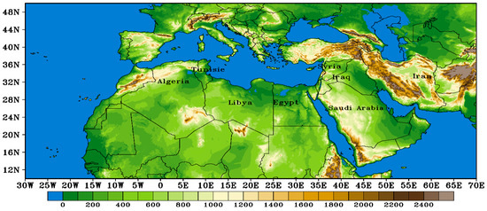
Figure 1.
Longitudinal–latitudinal geographical maps of the study area. Shaded areas represent the surface topography.
Figure 2 and Figure 3 present detailed analyses of the geopotential height (represented by contour lines) and temperature (indicated by color shading) at two atmospheric levels, 1000 and 500 hPa respectively. The data span the period from 26 January to 4 February 2006 and are crucial for understanding the spatiotemporal evolution of a Mediterranean cyclone during this time. The genesis of this Mediterranean cyclone occurred at the surface, with a system of low-pressure developing over the Atlantic Ocean off the IP at 12Z26 January (Figure 2a). This initial cyclogenesis was a surface-driven process. A key factor in the cyclone’s subsequent development was its interaction with an upper-level trough. Around January 29, this upper-level trough shifted southward and merged with the surface low. This convergence was crucial, leading to the instant growth of the cyclone at the surface and the formation of a robust Mediterranean cyclone. This intensified system then tracked eastward across the Mediterranean, maintaining its strength and deepening over the next four days. The cyclone’s weakening phase began toward the end of 3 February, resulting in a shallow depression by 00Z04 February. The system finally dissipated by 12Z04 February 2006.
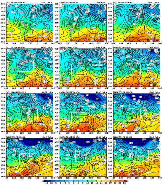
Figure 2.
The geopotential height distribution at 1000 hPa (solid line), with contours every 20 gpm, and the temperature (shaded-°C) for the period from 12Z27 January to 12Z04 February 2006.
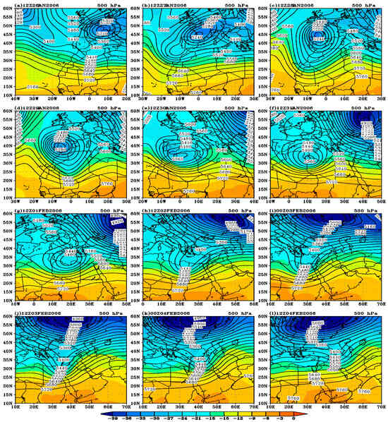
Figure 3.
The geopotential height distribution at 500 hPa (solid line), with contours every 40 gpm, and the temperature (shaded-°C) for the period from 12Z27 January to 12Z04 February 2006.
As shown in Figure 2a, the midlatitude cyclone was located at the surface over the North Atlantic Ocean at 12Z26 January. The figure also depicts high pressure dominating much of the region, with a high-pressure system over Northern Europe and a subtropical high influencing the western part. The cyclone itself was positioned between these high-pressure systems, off the western coast of the IP. The cyclone gradually deepened and moved eastward, as the high-pressure system retreated southwestward, allowing the low-pressure system to advance slightly southward (Figure 2b). This pattern persisted through 28 January, with the low continuing its eastward movement over the northern part of Algeria. Meanwhile, in the upper atmosphere, the contour lines are nearly straight and parallel in the southern half of the domain. The northeastern part is dominated by a cutoff low, centered over Western Europe, where the geopotential height reaches approximately 5240 (Figure 3a). After 24 h, influenced by the polar jet stream, this trough began to move southwestward. This polar jet supplied the trough with cold polar air, contributing to the deepening and strengthening of the cyclone (Figure 4b). By 12Z28 January, the jet stream’s influence was pronounced, with strong northerly winds pulling the cutoff low southward (Figure 3c and Figure 4c).
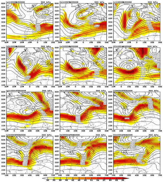
Figure 4.
The geopotential heights (lines) and wind speeds (shaded areas) at 300 hPa, with a minimum speed of 30 m/s for the period from 12Z27 January to 12Z04 February 2006.
At 12Z29 January 2006, the merging of the cyclone at the surface and the cutoff low at the upper level occurred over the western Mediterranean Sea (Figure 2d and Figure 3d). A key factor in this amalgamation was the influence of the polar jet stream. Its strong northerly winds, characterized by cold, dense air and exceeding 60 m/s (Figure 4d), provided the dynamic force necessary to bring the two cyclone centers together. This system also exhibited a characteristic westward tilt, with the 500 hPa cyclone center positioned west of the 1000 hPa center. Approximately 24 h later, the strong, cold polar jet stream merged with the subtropical jet stream (Figure 2e, Figure 3e and Figure 4e). This merged jet stream then advected the cyclone eastward. Simultaneously, a thermal ridge developed over the southern portion of the domain. By 12Z31 January 2006, the cyclone had reached the northern coast of Libya (Figure 2f and Figure 3f). The northward-advancing thermal ridge then encountered the cold air associated with the cyclone. This collision created a region of significant baroclinic instability, which, in turn, contributed to the cyclone’s further intensification. This dynamic situation persisted for the subsequent 24 h, as illustrated in Figure 2g and Figure 3g.
By 2 February 2006, the Mediterranean cyclone began to weaken, primarily because of the diminished supply of the cold, polar air, as evidenced by the geopotential height values. The polar jet stream’s transport of the cold air from the pole had effectively ceased. However, despite this reduction in the cold air source, a significant temperature difference persisted across the cyclone, both in the upper air and at the surface (Figure 2h and Figure 3h), suggesting that other factors were contributing to its dynamics. Concurrently, the Red Sea trough (coincides with the Sudan monsoon low) expanded significantly, encompassing the Red Sea region and southeastern Egypt (Figure 2h). A thermal gradient, linked to the Red Sea trough, stretched zonally across northern Sudan and the southern Arabian Peninsula (AP), further highlighting this complex thermal environment. Figure 3h shows the simultaneous enhancement of an upper air trough above southeastern Italy and the northern coast of Libya, extending into northern and central Libya and appearing as an inverted trough.
As the monsoon strengthened in Sudan, the Red Sea trough began a gradual northward movement around 00Z03 February. The trough extended across much of Egypt and was linked to a thermal ridge, which formed a component of the surface baroclinic zone along the southern Mediterranean coast. At the same time, the subtropical high started to weaken and shifted a little to the east (Figure 2i), and a surface disturbance developed 12 h later. The interaction between warm and cold air masses caused significant instability over the eastern Mediterranean and western Saudi Arabia. Although the cyclone’s center was located over northern Saudi Arabia and the eastern Mediterranean during its final day (4 February), the temperature gradient increased, especially in the lower layers. Additionally, the upper-air trough at 500 hPa moved eastward, extending over northern and northwestern Egypt. By 00Z04 February, the surface cyclone had shifted northeastward, encompassing the northeastern AP and the eastern Mediterranean (Figure 2j). Finally, at 12Z04 February, the surface cyclone moved northeastward, while the upper-air trough vanished and became zonally flat (Figure 2l and Figure 3l). The upper-level trough and the surface cyclone were closely related from the beginning of the cyclone’s creation to its end, according to the geopotential height and temperature analyses at 1000 and 500 hPa (Figure 2 and Figure 3).
The polar and subtropical jet streams have maximum speeds of approximately 300 hPa and 200 hPa, respectively. Figure 4 demonstrates the distribution of wind speeds greater than 30 m/s at 300 hPa from 12Z26 January to 12Z04 February 2006, showing the behaviors of the polar and subtropical jets during this period. On January 26 and 27, 2006, the jet stream in the polar regions extended to the northern coast of Africa, coinciding with the cyclone’s entry into central Western Europe, influenced by cold air from the northeast. As the polar jet migrated southeastward, its maximum speed rose, topping 65 m/s at 300 hPa and 55 m/s at 200 hPa (Figure 4b). By January 28, the polar jet’s extension reached the cyclone’s center, with northerly winds exceeding 60 m/s (Figure 4c). During these three days, the subtropical jet stream weakened at 300 hPa. However, at 200 hPa, its core exceeded 50 m/s and moved eastward. This eastward shift at 200 hPa allowed the cyclone to deepen southward because of the influx of the northern cold air. From January 29 to 31, the polar jet drifted southeast and merged with the subtropical jet. Its maximum speed exceeded 60 m/s at 300 hPa (Figure 4d,e). At 200 hPa, during this period, the subtropical jet stream’s speed increased to approximately 60 m/s, which facilitated the cyclone’s rapid eastward movement. The complete merger of the polar jet’s extension with the subtropical jet over North Africa occurred between 12Z30 and 12Z31 January, during which time the polar jet’s extension gradually weakened at 300 hPa. The cyclone’s center was located at approximately 10°W at 12Z29 January and at 20°E at 12Z01 February. Toward the end of this period, an extension of the polar jet stream developed in the northeastern part of the domain, which acted to slow the cyclone’s eastward movement. By 12Z02 February, with the cyclone advancing southward and the cold air supply from the north weakening, the cyclone entered the edge of the subtropical region (Figure 4h) and began to weaken. The cutoff low disappeared, becoming an inverted trough, which persisted until the end of the study period. With a core exceeding 60 m/s at 300 hPa, the subtropical jet was located across northeast Africa, encompassing Libya and Egypt, and shifted slightly eastward. From 12Z02 to 1204 February, the subtropical jet stream strengthened, with its speed increasing to 65 m/s. This explains the trough’s rapid eastward movement from 20°E to approximately 50°E in just two days. The subtropical jet’s intensity gradually recovered to its typical distribution in terms of both speed and direction. At 200 hPa, the subtropical jet stream’s extension had a core of over 70 m/s, and wind direction over North Africa was zonal.
3.2. Analysis of Satellite Data
Figure 5 presents SEVIRI satellite images from the Meteosat Second-Generation (MSG) satellite, showing the spatial distribution of clouds and dust particles during the Mediterranean cyclone at six different times. The satellite imagery revealed extensive cloud cover over the cyclone, along with a dust plume associated with its southern flank. On January 30, the cyclone migrated to the southern Mediterranean and North Africa, generating strong surface winds that resulted in a storm over the central Mediterranean, especially impacting Italy and its surrounding areas (Figure 5a).
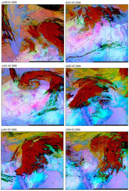
Figure 5.
MSG SEVIRI-derived false-color images over NA, showing dust (pink/purple), clouds (brown/orange), and differences in surface emissivity retrieved in the absence of dust or clouds (light blue/blue) on (a) 30 January 2006, (b) 31 January 2006, (c) 01 February 2006, (d) 02 February 2006, (e) 03 February 2006, and (f) 04 February 2006. (https://meteologix.com/eg/satellite/; accessed on 15 March 2025).
The cyclone’s movement and deepening coincided with increased dust emissions, driven by strong westerly winds from a cold air mass over central Libya (Figure 5b). By the next day, the cyclone was visible in satellite images as a complex system. The system, as depicted in Figure 5c, featured a curved band of clouds over the Mediterranean Sea, a spiral band of dust over northeastern Libya, and a linear band of dust extending eastward to western Egypt. The eastward migration of the cyclone brought strong winds to its southern side. These winds, continued to generate dust storms over eastern Egypt and the southeastern Mediterranean lands, accompanied by dense cloud cover on 2 February (Figure 5d). On 3 February, strong winds and various weather phenomena were recorded at most stations in Saudi Arabia. On this day, a dense dust and a cloud structure covered northern and central Arabia and much of the area east of the Mediterranean (Figure 5e). On 4 February, following the depression’s passage, the AP was clear of clouds, while dense clouds shifted eastward, indicating the storm’s conclusion and the cyclone’s dissipation (Figure 5f).
Figure 6 presents the geographical distribution of the TRMM’s daily rainfall during the study period. A comparison of Figure 5 and Figure 6 indicates a strong connection between the cloud cover observed in the satellite images and the rainfall data.
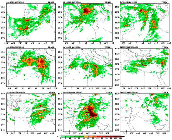
Figure 6.
The spatial daily rainfall pattern of the TRMM data for the period from 27 January to 4 February 2006.
Rainfall amounts were linked to the cyclone’s location and concentrated on its eastern side because of the upward vertical motion. The highest rainfall amounts occurred on 3 February, with some areas in Saudi Arabia recording thunderstorms and strong winds (Figure 6). This was because of the formation of a highly unstable atmospheric zone above the Red Sea region and the northern AP. Instability, leading to significant rainfall, resulted from warm, humid air advection by southeast monsoon winds and a cold air outbreak, driven by the upper-level cyclone, interacting between the polar and tropical air masses.
The precipitation patterns in Figure 5 and Figure 6 align with the typical distribution associated with rapid deepening in the “self-development paradigm” (heavy precipitation poleward and westward of the cyclone’s center). The release of latent heat during condensation and precipitation processes acts as a significant internal energy source for an extratropical cyclone. This diabatic heating directly warms the atmospheric column, increasing its thickness and lowering surface pressures hydrostatically. This warming, therefore, contributes to the available potential energy of the system, which can then be converted to kinetic energy [72]. Studies of rapidly intensifying cyclones have consistently highlighted that the integrated effects of latent heat release can represent a substantial component of the storm’s overall energy budget. This directly contributes to its intensification beyond what would be expected from purely adiabatic baroclinic processes alone [73,74,75,76]. This added energy not only contributes to the maintenance of the cyclone but also can play a crucial role in its deepening phase. This strongly suggests that latent heat release was, indeed, a key contributor to the intensification of this cyclone.
Latent heat release during cloud formation, particularly within the warm conveyor belt and other ascent regions of a cyclone, plays a critical role in modifying the atmospheric static stability, thereby enhancing vertical motion [73]. As condensation occurs, the released heat warms air parcels, increasing their buoyancy relative to that of the unsaturated environment or reducing the environmental lapse rate toward a moister adiabatic profile [77]. This reduction in the static stability makes it easier for air to ascend, leading to stronger and more focused upward vertical velocities. This process is particularly effective ahead of cold fronts or within the warm sector. Latent heating concentrated at lower and mid-levels can generate significant positive potential vorticity anomalies below the level of the maximum heating, which, in turn, induce cyclonic circulation and further enhance organized ascent [78,79]. The influence of the latent heat release extends beyond direct energy input and stability modification; it is a key component of the “self-development” paradigm in cyclone intensification, a process where positive feedback loops amplify the storm’s growth [73]. In this paradigm, as latent heat release enhances the vertical motion and deepens the surface low, the strengthened cyclonic circulation can increase low-level moisture convergence by drawing in more moist air from the boundary layer. This enhanced moisture supply then fuels further condensation and latent heat release, creating a feedback loop that promotes continued, and often rapid, intensification [80,81]. Furthermore, diabatic heating can strengthen thermal gradients and frontogenesis, thereby enhancing the baroclinic processes that also drive the cyclone. The strategic location of the heavy precipitation, such as that observed poleward and westward of our cyclone’s center (Figure 5 and Figure 6), is often associated with self-development. This is because it can efficiently contribute to the generation of cyclonic vorticity and the overall deepening of the system [82].
3.3. Analysis of Temperature Advection
Winter weather in the Mediterranean region is often disrupted by traveling cyclones, which typically form southwest of Europe when the associated trough extends southward over northwest Africa (Figure 2 and Figure 3). To assess the cyclone’s evolution and its associated weather patterns, we analyzed the temperature advection at 850 hPa from 12Z26 January to 12Z04 February 2006. The temporal development of the temperature advection (cooling/heating) and geopotential height distribution within the cyclone’s influence area at 850 hPa is visualized in Figure 7. The analysis shows a warm air advection zone east of the 850 hPa trough, indicating a warm sector, and a cold air advection zone west of the trough, indicating a cold sector. Additionally, Figure 7 illustrates the eastward tracking of both the warm and cold advection regions, coinciding with the cyclone’s trajectory. A comparison of Figure 7 with Figure 2 and Figure 3 shows that the region west of the trough, characterized by descending motion [62], corresponds to cooling. Conversely, the eastern region of the trough, characterized by ascending motion, is associated with warming. Hence, heating is typically associated with rising motion and cooling with descending motion. Figure 7 shows the temporal variations in the heating and cooling patterns over the study domain during the study period.
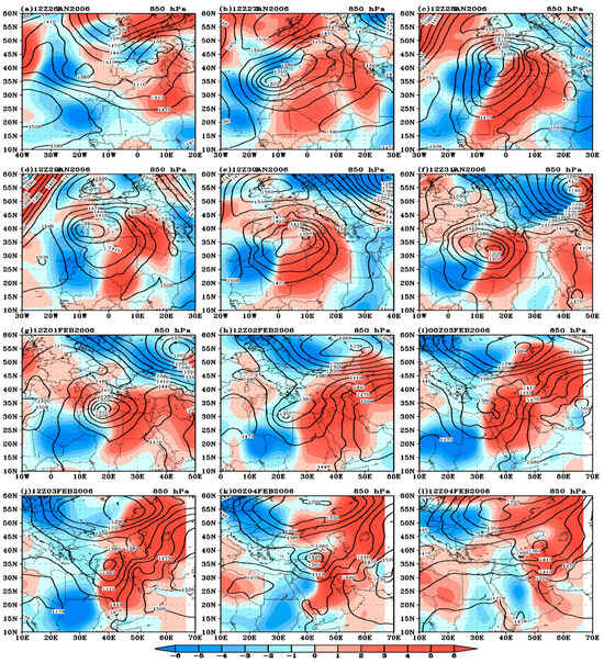
Figure 7.
The advection of the temperature (shaded) at 850 hPa, with geopotential height (lines), for the period from 12Z27 January to 12Z04 February 2006.
On 26 January, the cyclone appeared at the 850 hPa level as a weak cutoff low. Strong cold advection covered the cyclone’s western region, with the maximum values in two areas: one, the strongest cooling, in the mid-Atlantic Ocean, and the other, more widespread, off the west coast of Africa (Figure 7a). Warm advection on the cyclone’s eastern side was relatively weak, though stronger over the Sahara Desert in North Africa. Twenty-four hours later (Figure 7b), the cyclone’s center had deepened, and the geopotential height had decreased. A region of strong cold advection developed west of the cyclone, coinciding with the influx of cold air accompanying the polar jet stream. Conversely, on the cyclone’s eastern side, as it moved eastward, warm advection became more pronounced, with higher values than those previously observed. This pattern persisted until 28 January. Figure 7c shows that both cold and warm advection values were higher than those previously observed, each covering a nearly equal area. The trough line and front were clearly defined. The cyclone covered a very large area, nearly the largest during the study period, as shown by the horizontal distribution of the geopotential height contours. The cold air associated with this traveling cyclone reached North Africa across the Mediterranean Sea.
Twenty-four hours later, both the cold and warm advections weakened. High pressure in the northern part of the domain pushed the cyclone southward, transferring heat from its eastern side to its northern side (Figure 7d). This pattern persisted until 30 January, by which time the cold advection had shrunk to the cyclone’s southwestern corner, and the cyclone’s center had moved eastward (Figure 7e). By 31 January, the cyclone’s center was located over northern Libya. Strong warm advection prevailed east of the cyclone because of heating from the desert, while the advection north of the cyclone, and the associated cooling, weakened as the supply of the cold air diminished (Figure 7f). The cyclone’s center shifted slightly eastward on 1 February, with the associated cold and warm advection patterns moving in tandem. As shown in Figure 7g, warm advection weakened in the north, allowing cold air to leak southward and create a channel that fed cold air to the cyclone’s center. By 2 February, the cyclone under study had weakened considerably, while a more potent cyclone to the northeast gained dominance.
Figure 7h shows increased warm advection dominating a large area. This is consistent with the transport of the warm, moist air northward from the tropics by the extended Red Sea trough and the advection of significant cold air southward from the polar region by the upper-level trough (Figure 7h–j). The atmospheric instability over the AP was intensified by the interplay of the polar and tropical air masses. This gradient (between the cold and warm air), combined with the cyclone’s eastward movement, intensified the low-level baroclinicity. A low-level baroclinic area, demarcated by a pronounced thermal gradient, was extant over North Africa. This substantial horizontal thermal gradient (Figure 7) fulfilled the requisite conditions for baroclinic instability, as delineated by [83]. On 3 February, the area of the cold advection increased, as did the strength of the warm advection. This increased the instability over this and neighboring regions, as the interaction between the different air masses continued. This pattern persisted until the end of the day, with marked decreases in both cold and warm advections. After 00Z04 February, the Red Sea trough shifted southeastward (Figure 7k,l), while the upper-air trough shifted northeastward, breaking their connection. Consequently, the region came under the influence of a high-pressure system, leading to atmospheric stability.
3.4. Isobaric Relative Vorticity Analysis
The significant impact of the cyclogenesis over the Mediterranean and North Africa on weather conditions, specifically, strong winds, precipitation, and temperature drops, has led to extensive research on this subject [58,62,66,67,84,85,86]. The close relationship between cyclogenesis and local weather forecasting necessitates a detailed understanding of cyclogenesis characteristics in this region. Throughout the study period, Figure 8 shows the relative vorticity distribution at 850 hPa, highlighting a dynamically evolving cyclonic circulation. This evolution is characterized by changes in the magnitude, orientation, and horizontal extent of the relative vorticity, which reflect the cyclone’s growth, movement, and eventual dissipation. At 12Z27 January 2006, Figure 8a reveals two weak relative vorticity cells, one linked to the nascent upper-level cyclone and the other to the surface cyclone centered over the North Atlantic Ocean. The surface cyclone strengthened and shifted slightly southeast over the next 24 h (Figure 8b), centering at around 35° N and 10° W, as the upper-level cyclone also tracked southward.
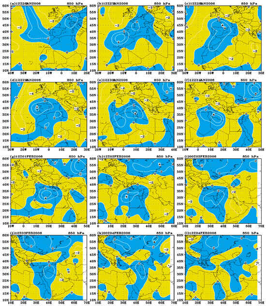
Figure 8.
An 850 hPa relative vorticity with an interval of 2 × 10⁻⁴
s−1. Solid (dashed) lines represent positive (negative) values for the period from 12Z27 January to 12Z04 February 2006.
At 12Z28 January, the two vorticity cells merged, forming a large single cell centered at around 5° W and extending from 50° N to 30° S (Figure 8c). Twenty-four hours later (Figure 8d), the two cyclones had fully combined, resulting in a single, stronger cyclone with a prominent inner cell centered at 40° N and 10° W. The center of the maximum relative vorticity shifted northeastward to 35° N, 10° E by 12Z30 January 2006 (Figure 8e). Over the following 24 h (12Z31 January), the positive relative vorticity cell continued its eastward movement, with an increase in its maximum value (Figure 8f). The period from 12Z01 to 00Z03 February saw the center of the maximum relative vorticity track continuously eastward, contracting and weakening as the upper-level depression weakened (Figure 8g–i). The positive relative vorticity cell continued northeastward, aligning with the surface cyclone over northwest Egypt by the end of this period. The magnitude of the relative vorticity decreased as the cyclone moved north of the AP and the eastern Mediterranean (Figure 8j). Concurrently, the positive relative vorticity cell shifted to southern Iraq, with its maximum value decreasing (Figure 8k).
A crucial finding of this study is the observed close spatial and temporal consistencies between the surface cyclone’s center, identified at 1000 hPa, and the maximum positive relative vorticity’s center, at 850 hPa. This alignment provides strong evidence of a robust vertical linkage throughout the cyclone’s lifecycle. Such strong coupling is entirely consistent with established dynamic principles governing cyclogenesis. For instance, mechanisms such as boundary layer pumping, which influences low-level convergence, and the impact of the upper-tropospheric divergence are well known to significantly affect the sea-level pressure and low-level vorticity’s tendencies (Hoskins et al., 1985 [87]; Martin, 2013 [88]). These fundamental processes, therefore, explain how the cyclone’s surface manifestation is dynamically tied to, and influenced by, the vorticity structure in the overlying lower troposphere, such as that at the 850 hPa level, demonstrating a deeply coupled atmospheric system from its formation through its mature stages. Furthermore, the positive relative vorticity values at 00Z were generally higher than those at 12Z, while the horizontal extent of the positive relative vorticity’s center was greater at 12Z than at 00Z.
3.5. Analysis of the Atmospheric Kinetic Energy Budget
The AKE, derived from the conversion of the AAPE and dissipated through frictional processes, plays a pivotal role in maintaining the strength and characteristics of the general circulation. Therefore, understanding the generation and dissipation of the AKE is essential for comprehending the fundamental processes of the atmospheric energy cycle and the dynamics of large-scale atmospheric systems. The regional balance of the AKE, comprising the horizontal flux, adiabatic generation, and frictional dissipation, plays a crucial role in the development of atmospheric phenomena at various scales. Studies by Abdeldym et al. [58] Al-Mutairi et al. [66], Alkhouly et al. [67], Labban [55], and Morsy et al. [89] have underscored the significance of these key terms. To investigate the energetics of the cyclonic system, a detailed AKE budget analysis was performed. Using Equation (3), the individual terms of the budget were calculated for a defined volume extending vertically throughout the troposphere, from the 1000 hPa pressure level (near the surface) up to the 100 hPa level. The analysis focused on a dynamic field encompassing the cyclonic circulation, delineated by the box shown in Figure 2. The AKE budget, expressed in Eulerian form, was computed for the period spanning from 29 January 2006 to 4 February 2006. This specific timeframe was selected because it captures the cyclone’s critical lifecycle stages, from the initial merging of the surface and upper-level depressions to the system’s eventual dissipation. Table 1 illustrates the time-averaged AKE budget components for the cyclonic system across various isobaric levels. Throughout the cyclogenesis event’s lifecycle, the dominant AKE source was the persistent activity of the upper-tropospheric jet stream. Notably, the peak AKE generation occurred between 500 hPa and 150 hPa, coinciding with the proximity of the strong polar and subtropical jet streams. The local rate of the change in the AKE indicated a temporal decrease in the average AKE at levels below 500 hPa, as well as at 250 hPa, 200 hPa, and 100 hPa, while increases were observed at 400 hPa, 300 hPa, and 150 hPa.

Table 1.
Temporal mean of area average for atmospheric kinetic energy (104 J/m2) and AKE budget terms (W/m2) at standard pressure levels.
Within the mid- to upper troposphere (700–150 hPa), the horizontal flux of the AKE demonstrates a significant transport of the AKE to the computational domain, with the maximum values observed near the jet stream level (400–200 hPa). Conversely, in the boundary layer, this term acts as an AKE sink, effectively transporting the AKE out of the computational domain. The vertical transport of the AKE is downward when positive (300–100 hPa) and upward when negative (1000–400 hPa) [58,90,91,92]. Upward transport acts as an AKE source for the upper troposphere/stratosphere and a sink for the lower/middle troposphere. The AKE generation pattern observed is consistent with findings from prior research [55,58,66,67]. In the boundary layer, a slight destruction of the AKE, representing its conversion to the AAPE, is observed. This phenomenon is primarily because of a large region of downgradient flow situated ahead of the major baroclinic trough extending into the subtropical high. Conversely, the upper troposphere exhibits strong AKE generation. This generation is attributed to the interaction between the wind speed and cross-contour flow. In the lower troposphere, the limited angle between the flow and geopotential height contours results in negative generation values. However, in the upper troposphere, the high magnitude of the wind speeds creates a substantial region of strong AKE generation. Although the upper-tropospheric wind field is mostly shaped by the geostrophic balance, relatively small ageostrophic deviations from this balance are dynamically critical. In regions like jet streams and developing waves, where pressure gradients and wind speeds are high, these systematic ageostrophic components are highly effective at generating a substantial AKE. Even if representing only 10–20% of the total wind, they facilitate flow across strong geopotential gradients toward lower pressures. This AKE generation is captured by the term . Even when V is mostly parallel to contours, a very high V with even a slight angle across them can result in high AKE generation.
The dissipation term exhibits contrasting behaviors across different atmospheric layers. In the lower troposphere (1000–700 hPa), it consistently acts as an AKE source (positive dissipation), a finding supported by prior research [58,66,93,94]. This subgrid-to-grid energy transfer is likely because of convection and turbulence, though their precise mechanisms are not fully understood [95]. Above 500 hPa, however, the dissipation term shifts to an AKE sink (negative dissipation), peaking at jet stream levels. The underlying subgrid-to-grid energy transfer processes, again likely involving convection and turbulence, remain elusive [95]. Computational uncertainties in residual terms must be considered. A comparison of the external (HFKE) and internal (GKE + DKE) sources/sinks [54] shows external/internal dominance above/below 400 hPa.
To elucidate the dynamic mechanisms governing the cyclone’s formation and evolution during the study period, the volumetric mean of the AKE was computed for each time step. Additionally, a thorough AKE budget analysis was conducted, quantifying the various sources and sinks of the AKE within the computational domain. This integrated approach facilitated a detailed evaluation of the dynamic processes contributing to the cyclone’s development. The volumetric means of the AKE and AKE budget terms, calculated at six-hour intervals (four times daily), are presented in Table 2. Notably, the vertical flux of the AKE is omitted from Table 2 because of the solid boundary condition on the vertical motion (omega), which results in a zero integral. Table 2 demonstrates the robust dynamic relationship between the AKE and the polar and subtropical jet streams. The temporal fluctuations in the AKE (Table 2) are in close alignment with the changes in the jet stream’s intensity (Figure 4). Notably, increased jet stream activity corresponds to higher AKE levels, while decreased jet stream activity correlates with lower AKE levels, indicating a substantial modulation of the AKE by the jet streams. The period from 00Z29 to 12Z30 January saw a gradual rise in the AKE, coinciding with the polar jet’s midlatitude extension and merger with the subtropical jet (Figure 4). A further AKE increase, from 06Z31 January to the end of February 3, correlated with the continued jet stream’s activity. The peak AKE, at 18Z02 February, matched the subtropical jet’s maximum intensity. As the cyclone weakened and moved beyond the jet stream’s influence, the AKE decreased. The rate of the change in the AKE, reflecting instantaneous AKE variations, tracked the overall AKE trends, changing signs to indicate increases (positive) or decreases (negative). Table 2 shows a peak rate of change of 2.83 W/m2 during the initial AKE increase (29–30 January). A significant AKE decline and a corresponding decrease in the rate of change occurred toward the end of the study.
Table 2.
Area-averaged vertical mean for atmospheric kinetic energy (104 J/m2) and AKE budget terms (W/m2) for the cyclonic system.
The observed cyclonic development is consistent with classical baroclinic theory, originally formulated by [96] and subsequently expanded upon by Kung and Baker [97]. This conformity is primarily because of the dominant influence of the AKE generation term within the energy budget, which acts as a crucial diagnostic for delineating the cyclone’s lifecycle stages. Initially, negative AKE generation values indicate AKE conversion to the AAPE as the cyclone moves from low to high geopotential heights. This aligns with baroclinic instability theory, driven by temperature gradients and wind shear [98]. The polar jet enhances cyclone intensification by providing additional energy. As the cyclone deepens, AKE generation increases, becoming positive and proportional to the cyclone’s strength. This relationship is documented in midlatitude cyclone studies, using generation as a diagnostic tool [58,91,92,99,100]. Negative AKE generation values in the first six time-steps indicated AKE-to-AAPE conversion. Starting at 12Z30 January, positive values signaled a shift to AAPE-to-AKE conversion, driven by air mass movement from high to low pressure, consistent with the findings of Hoskins et al. [87]. The boundary values during this positive phase ranged from 2.7 W/m2 to 87 W/m2. This period is divided into two distinct sub-periods: The first, from 12Z30 January to 12Z01 February, features a gradual decline in positive AKE generation term values, attributed to a reduction in the cold air supply, which weakens the system [101]. The second, from 18Z01 February to the end, shows a significant increase in boundary values, peaking because of the cyclone’s northward trajectory and associated robust energy conversion. This observed behavior is consistent with the theoretical framework of baroclinic instability, as outlined by Kung and Baker [97], and emphasizes the dynamic interaction between energy conversion processes and cyclone intensification. Furthermore, recent studies employing high-resolution models and reanalysis data [102] have provided additional empirical support for the critical role of baroclinic processes in driving cyclonic development.
The horizontal flux of the AKE acted primarily as an AKE source throughout the study, with the most substantial contributions occurring during the cyclone’s development, from 06Z30 January to 12Z01 February. The consistently positive values indicate a net AKE inflow, which is vital for maintaining and strengthening the cyclone. The dominance of this term is explained by the inflow jet’s initial strength, which significantly exceeded the outflow jet’s strength during this phase. This asymmetry is typical of baroclinic systems, where the inflow jet is instrumental in transporting energy into the cyclone, as shown in studies by Hoskins et al. [87]. As the study progressed, a gradual weakening of the inflow jet, especially in the western domain corner, caused a nearly consistent decrease in the horizontal flux term, with the most pronounced decline in the final three time-steps. This reduction in the jet’s strength is associated with diminishing baroclinic forcing and temperature-gradient decreases, key drivers of jet stream dynamics [98]. This behavior is in agreement with the findings of Novak et al. [102], who observed that the weakening of the inflow jet during the decay phase of midlatitude cyclones is correlated with a reduction in the horizontal AKE flux. The observed trends in the horizontal AKE flux term are consistent with the theoretical framework of energy budgets in cyclonic systems, as described by [99,100], which emphasize the importance of the horizontal AKE transport for maintaining cyclone intensity, particularly during its development. The gradual decrease in the horizontal flux term during the later stages of the study reflects the cyclone’s transition to a mature or decaying phase, where the energy inputs from the inflow jet are no longer sufficient to sustain the system’s intensity [101].
Despite ongoing AKE generation, significant dissipation leads to a net internal AKE loss. As evidenced by Table 2, the dissipation term peaks alongside the generation term’s maximum intensity, revealing a dynamic balance between energy production and dissipation, typical in multiscale atmospheric systems. Interestingly, smaller-scale waves consistently dampen, unlike larger-scale waves, because of stable flow conditions that suppress subgrid perturbations and promote energy transfer to larger scales. The simultaneous increases in the horizontal flux and cross-contour flow, coupled with enhanced dissipation, demonstrate the complex interplay between energy sources and sinks. Specifically, the horizontal flux and generation are the main AKE sources, while dissipation is the dominant sink. This balance prevails for most of the study, except for the first six time-steps. In this initial phase, dissipation acts as the primary AKE source, with energy transferring from smaller to larger scales. This aligns with energy upscaling, where subgrid processes amplify larger-scale motions. The data presented in Table 2 clearly establish the dominance of the external source, attributed to the jet stream’s activity, in governing the processes within the studied region throughout the entire study. This external source consistently acts as an AKE source, while the internal processes act as an AKE sink.
A more comprehensive understanding of cyclone dynamics requires further investigation. This analysis uses vertical–temporal cross-sections (Figure 9) to explore the cyclone’s vertical structure and temporal evolution. Figure 9a illustrates a persistent upper-level jet stream (500–150 hPa) within the cyclogenesis zone, a key feature that provides the necessary energy and momentum for cyclone intensification throughout its lifecycle. Over time, the layer of the maximum energy gradually shifts upward as the cyclone progresses, moving from the polar jet stream region, which is centered at around 300 hPa at the beginning of the study period, to the subtropical jet stream region, centered at around 250 hPa during the mid-phase of the study, and eventually exiting this region by the end of the period. The analysis also reveals that the AKE exhibits three distinct peaks during the study period, each corresponding to specific phases of the jet streams’ interaction. The first peak occurs on 30 January, with an AKE value of approximately 140*104 J/m2, coinciding with the initial merger of the two jet streams. This merger enhances the baroclinic instability, leading to an increase in the AKE. The second peak, observed at 12Z31 January, occurs after the complete merger of the two jet streams and is similar in magnitude to the first peak. This phase represents a period of sustained energy input into the cyclone, driven by the combined influence of the merged jet streams. The third, and most significant, peak occurs during the intensification phase of the subtropical jet stream, reaching the highest AKE value observed during the study. This peak underscores the critical role of the subtropical jet stream in amplifying cyclonic activity, as it provides additional energy and momentum to the system. These findings align with and confirm earlier results, highlighting the importance of jet stream interactions in modulating cyclone development. The vertical–temporal cross-sections provide valuable insights into the energy distribution and transfer processes within the cyclone, emphasizing the role of upper-level dynamics in shaping its lifecycle.
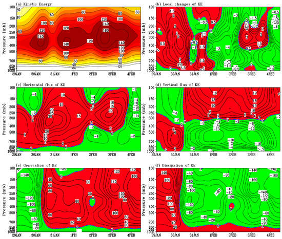
Figure 9.
Vertical–temporal profile of atmospheric kinetic energy (104 J/m2 (100 hPa) −1) and AKE budget terms (W/m2 (100 hPa) −1) for the cyclonic system.
Figure 9b illustrates the vertical and temporal patterns of the local rate of the change in the AKE, providing insights into its vertical and temporal variations throughout the study period. During the initial phase, from the beginning of the study until 00Z on February 1st, the rate of the change in the AKE was predominantly positive throughout the troposphere, except for in the boundary layer during the first three time steps. The maximum positive values were observed in the layers influenced by the polar jet stream (400–300 hPa), coinciding with the initial stages of the merger between the polar and subtropical jet streams. This merger enhanced the baroclinic instability, leading to an increase in the AKE within these layers. Following the merger, a notable shift occurred, with the rate of the change in the AKE transitioning from positive to negative values. This shift indicates a gradual decrease in the AKE throughout the troposphere over time, particularly in the upper layers between 400 and 500 hPa. This decline persisted until the end of the study period, with the exception of a brief interval from February 2nd to February 4th. During this interval, the rate of the change in the AKE became positive again within the pressure levels of approximately 400–150 hPa. This resurgence coincided with the intensification of the subtropical jet stream, which injected additional energy into the system during the final phase of the study. Around 3 February, a slight increase in the cyclone’s AKE was observed. This period marked the interaction and merger of the cyclone with the Red Sea trough, which contributed to enhanced atmospheric instability, particularly within the boundary layer. This interaction played a significant role in temporarily boosting the cyclone’s kinetic energy, highlighting the influence of regional atmospheric features on cyclonic activity.
As depicted in Figure 9c, the horizontal flux of the AKE primarily functions as a source of energy for the system throughout most of the study period, from the beginning until 12Z on 3 February. However, there are some notable exceptions: At levels below 850 hPa and above 200 hPa during the first four time-steps, the horizontal flux transitions to a weak energy sink. Additionally, within the layer between 850 hPa and 400 hPa, this term acts as an energy sink during the period from 18Z on 1 February to 18Z on 3 February. Furthermore, during the final three time-steps, the horizontal flux of the AKE becomes a sink of energy throughout the troposphere. The peak positive values of the horizontal flux term are concentrated between 400 hPa and 150 hPa, directly corresponding to the region of the jet stream’s strengthening. This correlation highlights the crucial role of jet streams in modulating the horizontal AKE flux. Specifically, the entrance and exit regions of jet streams are commonly associated with strong divergence or convergence zones in the horizontal flux, as noted by [103]. These dynamics emphasize the importance of the horizontal flux term for energy redistribution within the atmospheric system, particularly concerning the jet stream’s activity. The vertical AKE flux, as depicted in Figure 9d, displays contrasting patterns during the study. Between 00Z29 and 12Z30 January, upward AKE transport, indicated by negative flux values, dominates above 300 hPa, with the maximum intensity above 200 hPa. In contrast, downward AKE transport, shown by positive flux values, prevails between 1000 hPa and 400 hPa, peaking within the 700–500 hPa layer during the same timeframe.
The generation term, as depicted in Figure 9e, acts as a primary energy sink below 850 hPa for the duration of the study and at all the tropospheric levels during the first six time-steps. This signifies the conversion from the AKE to the AAPE during this phase. In the lower troposphere, adiabatic processes, specifically, cross-isobaric flow and frictional dissipation, are the dominant forces influencing the AKE, as noted by [104]. The generation term transitions to an AKE source above 850 hPa from 12Z30 January onward, driven by the work performed by the cross-isobaric flow. AKE generation occurs with flows toward low pressures, and AKE destruction occurs with flows toward high pressures. The generation term can also act as the dominant AKE sink during AKE-to-AAPE conversion. This dual role is supported by research on extratropical and tropical cyclones [58,66,91,92,105,106] which emphasizes the context-dependent complexity of energy conversion processes in these systems.
Figure 9f shows that the dissipation term functions uniquely within the boundary layer, consistently acting as a weak energy source throughout the study and at all the levels during the initial six time-steps. This suggests AKE production within these regions, likely because of subgrid-scale processes and frictional forces. Haimberger [107] explains this phenomenon, stating that the dissipation term can become an AKE source when subgrid-scale motion energy is converted to larger-scale motion energy. This aligns with findings from extratropical and tropical cyclone studies [58,66,91,92,105,106], showing the dissipation term can be an AKE source under specific conditions. Beginning at 12Z30 January and persisting until the study’s end, the dissipation term acts as an energy sink above 850 hPa, as indicated by negative values in Figure 9f. The observed energy losses are primarily because of eddy dissipation and viscous friction, which are typical of turbulent atmospheric flows. As expected, the dissipation term’s peak magnitude coincides with the cyclone’s maximum intensity, reflecting the increased energy dissipation during stronger cyclonic activity. This correlation underscores the context-dependent dual role of the dissipation term, which can act as either a source or a sink of the AKE according to the motion scale, cyclone intensity, and dominant physical processes.
The AKE budget analysis offers a powerful quantitative framework for understanding cyclone dynamics by explicitly linking energetic transformations to specific atmospheric processes. For instance, the energetic impact of ageostrophic flows, particularly those associated with the jet stream, is directly quantified by AKE budget terms, such as generation by cross-contour flow and the conversion of the AAPE through cross-isobaric flow. These terms precisely measure how the non-geostrophic components of the flow, which are fundamental drivers of upper-level divergence and convergence patterns critical for cyclone development, contribute the AKE to the storm system. Results showing that generation was a dominant energy source and that jet activity was a principal driver of the AKE underscore the budget’s utility in confirming and quantifying the well-known, but often qualitatively described, energetic importance of jet-related ageostrophic circulations in cyclogenesis. Furthermore, the AKE budget provides a concrete energetic measure of the crucial vertical coupling between surface and upper-level features characteristic of baroclinic development. The conversion of the AAPE to the AKE, directly related to vertical motions and thermal contrasts, quantifies the rate at which the potential energy stored in the atmosphere’s temperature gradients is converted to the AKE. This conversion process is the energetic manifestation of the interaction between surface fronts and upper-level troughs: As warm air rises and cold air sinks, the AAPE is released. Within the AKE budget, this conversion is typically quantified by the generation term, highlighting it as a primary energy source. Thus, AKE analysis provides a quantitative diagnosis of the strength and energetic consequences of this baroclinic coupling, moving beyond purely descriptive accounts of front–trough interactions.
4. Conclusions
This study utilized ERA5 reanalysis data to offer a thorough examination of the synoptic-scale evolution and dynamics of an intense Mediterranean cyclone that affected the Mediterranean region and the AP from 26 January to 4 February 2006. By examining the synoptic conditions, isobaric vorticity, temperature advection, and atmospheric kinetic energy budget, this research identified the key dynamic processes responsible for the cyclone’s formation and strengthening and the associated dust storm.
Behind the cyclone, cold air masses originating from higher latitudes were advected southward, leading to significant cooling over the Mediterranean regions. This cold advection contributed to increased atmospheric instability, promoting enhanced precipitation in these areas. Conversely, ahead of the cyclone, warm subtropical air was transported northward into the northern AP and eastern Mediterranean, resulting in elevated temperatures across the northern AP and the Levant regions. The interaction between these contrasting air masses played a crucial role in strengthening the cyclone, as the warmer, more buoyant air ascended over the denser cold air, fostering cloud development and precipitation. The pronounced temperature gradients contributed to increased baroclinic instability, a fundamental mechanism for cyclone intensification in midlatitudes. These temperature advection processes not only dictated precipitation patterns but also influenced wind regimes, leading to strong gusts and turbulent conditions across the affected regions. Additionally, upper-level atmospheric dynamics, particularly the presence of a jet stream, further enhanced the cyclone’s deepening by providing divergence aloft, which facilitated stronger upward motion and subsequent surface pressure drops. Vorticity analysis, in isobaric coordinates, reveals that the advection of the warm air mass and positive vorticity toward the developing cyclone played crucial roles in initiating its formation and the subsequent development of intense low-level winds.
The AKE and budget term analysis reveals that the continuous activity of the jet streams in the upper level served as the principal driver of the AKE throughout the lifecycle of this Mediterranean cyclone. The concentration of the majority of the AKE was between 500 and 200 hPa, which corresponded to the time of the high jet stream activity during cyclogenesis. The conversion of the AAPE, which was made possible by cross-isobaric flows toward areas of lower pressure, was the main cause of the rise in the kinetic energy. Cross-contour flow, which generated kinetic energy, emerged as a dominant energy source during the cyclone’s development, particularly ahead of upper-level troughs, where strong pressure gradients were present. Conversely, during the pre-cyclogenesis period, this term acted as a sink of energy. The main energy sink during the cyclogenesis process was AKE dissipation from grid to subgrid scales, contrasting with the pre-cyclogenesis phase, when AKE dissipation from subgrid to grid scales was essential. Notably, the spatial distribution of the AKE dissipation closely mirrored that of the AKE generation but with the opposite sign. Throughout the cyclone’s lifecycle, the horizontal flux of the AKE remained consistently positive, indicating that this term acted as a continuous source of energy, sustaining the cyclone’s intensity. These findings underscore the intricate balance of the energy conversion, dissipation, and transport mechanisms that govern the dynamics of Mediterranean cyclones, emphasizing the crucial roles of upper-level jet streams and pressure gradients in their evolution.
Funding
This research received no external funding.
Institutional Review Board Statement
Not applicable.
Data Availability Statement
The data supporting the findings of this article are included within the article.
Conflicts of Interest
The author declares no conflicts of interest.
References
- Reale, M.; Cabos Narvaez, W.D.; Cavicchia, L.; Conte, D.; Coppola, E.; Flaounas, E.; Giorgi, F.; Gualdi, S.; Hochman, A.; Li, L.; et al. Future projections of Mediterranean cyclone characteristics using the Med- CORDEX ensemble of coupled regional climate system models. Clim. Dynam. 2022, 58, 2501–2524. [Google Scholar] [CrossRef]
- Ulbrich, U.; Leckebusch, G.C.; Pinto, J.G. Extratropical cyclones in the present and future climate: A review. Theor. Appl. Climatol. 2009, 96, 117–131. [Google Scholar] [CrossRef]
- Ulbrich, U.; Leckebusch, G.C.; Grieger, J.; Schuster, M.; Akperov, M.; Bardin, M.Y.; Feng, Y.; Gulev, S.; Inatsu, M.; Keay, K.; et al. Are greenhouse gas signals of Northern Hemisphere winter extratropical cyclone activity dependent on the identification and tracking algorithm? Meteorol. Z. 2013, 22, 61–68. [Google Scholar] [CrossRef]
- Zappa, G.; Shaffrey, L.C.; Hodges, K.I.; Sansom, P.G.; Stephenson, D.B. A Multimodel Assessment of Future Projections of North Atlantic and European Extratropical Cyclones in the CMIP5 Climate Models. J. Clim. 2013, 26, 5846–5862. [Google Scholar] [CrossRef]
- Pinto, J.G.; Karremann, M.K.; Born, K.; Della-Marta, P.M.; Klawa, M. Loss potentials associated with European windstorms under future climate conditions. Clim. Res. 2012, 54, 1–20. [Google Scholar] [CrossRef]
- Schwierz, C.; Köllner-Heck, P.; Mutter, E.Z.; Bresch, D.N.; Vidale, P.L.; Wild, M.; Schär, C. Modelling European winter wind storm losses in current and future climate. Clim. Change 2010, 101, 485–514. [Google Scholar] [CrossRef]
- Peixoto, J.P.; Oort, A.H. Physics of Climate; American Institute of Physics: College Park, ML, USA, 1992; 520p. [Google Scholar]
- Rudeva, I.; Simmonds, I.; Crock, D.; Boschat, G. Midlatitude fronts and variability in the southern hemisphere tropical width. J. Clim. 2019, 32, 8243–8260. [Google Scholar] [CrossRef]
- Sinclair, V.A.; Rantanen, M.; Haapanala, P.; Räisänen, J.; Järvinen, H. The characteristics and structure of extra-tropical cyclones in a warmer climate. Weather. Clim. Dyn. 2020, 1, 1–25. [Google Scholar] [CrossRef]
- Catto, J.L.; Ackerley, D.; Booth, J.F.; Champion, A.J.; Colle, B.A.; Pfahl, S.; Pinto, J.G.; Quinting, J.F.; Seiler, S. The Future of Midlatitude Cyclones. Curr. Clim. Change Rep. 2019, 5, 407–420. [Google Scholar] [CrossRef]
- Dacre, H.F.; Pinto, J.G. Serial clustering of extratropical cyclones: A review of where, when and why it occurs. Npj Clim. Atmos. Sci. 2020, 3, 48. [Google Scholar] [CrossRef]
- Catto, J.L.; Jakob, C.; Berry, G.; Nicholls, N. Relating Global Precipitation to Atmospheric Fronts. Geophys. Res. Lett. 2012, 39, L10805. [Google Scholar] [CrossRef]
- Hawcroft, M.K.; Shaffrey, L.C.; Hodges, K.I.; Dacre, H.F. How Much Northern Hemisphere Precipitation Is Associated with Extratropical Cyclones? Geophys. Res. Lett. 2012, 39, L24809. [Google Scholar] [CrossRef]
- Pfahl, S.; Wernli, H. Quantifying the relevance of cyclones for precipitation extremes. J. Clim. 2012, 25, 6770–6780. [Google Scholar] [CrossRef]
- Catto, J.L.; Pfahl, S. The Importance of Fronts for Extreme Precipitation. J. Geophys. Res. Atmos. 2013, 118, 10791–10801. [Google Scholar] [CrossRef]
- Hawcroft, M.K.; Shaffrey, L.C.; Hodges, K.I.; Dacre, H.F. Can Climate Models Represent the Precipitation Associated with Extratropical Cyclones? Clim. Dyn. 2016, 47, 679–695. [Google Scholar] [CrossRef]
- Nieto, R.; Ciric, D.; Vázquez, M.; Liberato, M.L.R.; Gimeno, L. Contribution of the main moisture sources to precipitation during extreme peak precipitation months. Adv. Water Resour. 2019, 131, 103385. [Google Scholar] [CrossRef]
- Befort, D.J.; Wild, S.; Knight, J.R.; Lockwood, J.F.; Thornton, H.E.; Hermanson, L.; Bett, P.E.; Weisheimer, A.; Leckebusch, G.C. Seasonal forecast skill for extratropical cyclones and windstorms. Q. J. R. Meteorol. Soc. 2019, 145, 92–104. [Google Scholar] [CrossRef]
- Hewson, T.D.; Neu, U. Cyclones, Windstorms and the IMILAST Project. Tellus Ser. A Dyn. Meteorol. Oceanogr. 2015, 6, 27128. [Google Scholar] [CrossRef]
- Roberts, J.F.; Champion, A.J.; Dawkins, L.C.; Hodges, K.I.; Shaffrey, L.C.; Stephenson, D.B.; Stringer, M.A.; Thornton, H.E.; Youngman, B.D. The XWS Open Access Catalogue of Extreme European Windstorms from 1979 to 2012. Nat. Hazards Earth Syst. Sci. 2014, 14, 2487–2501. [Google Scholar] [CrossRef]
- Kron, W.; Löw, P.; Kundzewicz, Z.W. Changes in risk of extreme weather events in Europe. Environ. Sci. Policy 2019, 100, 74–83. [Google Scholar] [CrossRef]
- Eiras-Barca, J.; Ramos, A.M.; Pinto, J.G.; Trigo, R.M.; Liberato, M.L.R.; Miguez-Macho, G. The concurrence of atmospheric rivers and explosive cyclogenesis in the North Atlantic and North Pacific basins. Earth Syst. Dyn. 2018, 9, 91–102. [Google Scholar] [CrossRef]
- Pradhan, P.K.; Liberato, M.L.R.; Ferreira, J.A.; Dasamsetti, S.; Vijaya Bhaskara Rao, S. Characteristics of different convective parameterization schemes on the simulation of intensity and track of severe extratropical cyclones over North Atlantic. Atmos. Res. 2018, 199, 128–144. [Google Scholar] [CrossRef]
- Seneviratne, S.I.; Nicholls, N.; Easterling, D.; Goodess, C.; Kanae, S.; Kossin, J.; Luo, Y.; Marengo, J.; McInnes, K.; Rahimi, M.; et al. Changes in climate extremes and their impacts on the natural physical environment. In Managing the Risks of Extreme Events and Disasters to Advance Climate Change Adaptation; A Special Report of Working Groups I and II of the Intergovernmental Panel on Climate Change, (IPCC); Field, C.B., Barros, V., Stocker, T.F., Qin, D., Dokken, D.J., Ebi, K.L., Mastrandrea, M.D., Mach, K.J., Plattner, G.-K., Allen, S.K., et al., Eds.; Cambridge University Press: Cambridge, UK; New York, NY, USA, 2012; pp. 109–230. [Google Scholar]
- Leonard, M.; Westra, S.; Phatak, A.; Lambert, M.; van den Hurk, B.; McInnes, K.; Risbey, J.; Schuster, S.; Jakob, D.; Stafford-Smith, M. A Compound Event Framework for Understanding Extreme Impacts. Wiley Interdiscip. Rev. Clim. Change 2014, 5, 113–128. [Google Scholar] [CrossRef]
- Zscheischler, J.; Martius, O.; Westra, S.; Bevacqua, E.; Raymond, C.; Horton, R.M.; van den Hurk, B.; AghaKouchak, A.; Jézéquel, A.; Mahecha, M.D.; et al. A Typology of Compound Weather and Climate Events. Nat. Rev. Earth Environ. 2020, 1, 333–347. [Google Scholar] [CrossRef]
- Raveh-Rubin, S.; Wernli, H. Large-scale wind and precipitation extremes in the Mediterranean: A climatological analysis for 1979–2012. Q. J. R. Meteorol. Soc. 2015, 141, 2404–2417. [Google Scholar] [CrossRef]
- Waliser, D.; Guan, B. Extreme Winds and Precipitation during Landfall of Atmospheric Rivers. Nat. Geosci. 2017, 10, 179–183. [Google Scholar] [CrossRef]
- Bloomfield, H.C.; Hillier, J.; Griffin, A.; Kay, A.L.; Shaffrey, L.C.; Pianosi, F.; James, R.; Kumar, D.; Champion, A.; Bates, P.D. Co-Occurring Wintertime Flooding and Extreme Wind over Europe, from Daily to Seasonal Timescales. Weather. Clim. Extrem. 2023, 39, 100550. [Google Scholar]
- De Luca, P.; Messori, G.; Pons, F.M.E. Dynamical systems theory sheds new light on compound climate extremes in Europe and Eastern North America. Q. J. R. Meteorol. Soc. 2020, 146, 1636–1650. [Google Scholar] [CrossRef]
- Poschlod, B.; Zscheischler, J.; Sillmann, J.; Wood, R.R.; Ludwig, R. Climate Change Effects on Hydrometeorological Compound Events over Southern Norway. Weather. Clim. Extrem. 2020, 28, 100253. [Google Scholar] [CrossRef]
- Owen, L.E.; Catto, J.L.; Stephenson, D.B.; Dunstone, N.J. Compound Precipitation and Wind Extremes over Europe and Their Relationship to Extratropical Cyclones. Weather. Clim. Extrem. 2021, 33, 100342. [Google Scholar] [CrossRef]
- Zhang, Y.; Sun, X.; Chen, C. Characteristics of Concurrent Precipitation and Wind Speed Extremes in China. Weather. Clim. Extrem. 2021, 32, 100322. [Google Scholar] [CrossRef]
- Catto, J.L.; Dowdy, A. Understanding Compound Hazards from a Weather System Perspective. Weather. Clim. Extrem. 2021, 32, 100550. [Google Scholar] [CrossRef]
- Martius, O.; Pfahl, S.; Chevalier, C. A global quantification of compound precipitation and wind extremes. Geophys. Res. Lett. 2016, 43, 7709–7717. [Google Scholar] [CrossRef]
- Messmer, M.; Simmonds, I. Global Analysis of Cyclone-Induced Compound Precipitation and Wind Extreme Events. Weather. Clim. Extrem. 2021, 32, 100324. [Google Scholar] [CrossRef]
- Ridder, N.N.; Ukkola, A.M.; Pitman, A.J.; Perkins-Kirkpatrick, S.E. Increased Occurrence of High Impact Compound Events under Climate Change. Npj Clim. Atmos. Sci. 2022, 5, 3. [Google Scholar] [CrossRef]
- Neu, U.; Akperov, M.G.; Bellenbaum, N.; Benestad, R.; Blender, R.; Caballero, R.; Cocozza, A.; Dacre, H.F.; Feng, Y.; Fraedrich, K.; et al. IMILAST: A community effort to intercompare extratropical cyclone detection and tracking algorithms. Bull. Am. Meteorol. Soc. 2013, 94, 529–547. [Google Scholar] [CrossRef]
- Petterssen, S. Weather Analysis and Forecasting, 2nd ed.; McGraw Hill: New York, NY, USA, 1956; Volume 1, 269p. [Google Scholar]
- Trigo, I.F.; Davies, T.D.; Bigg, G.R. Objective climatology of cyclones in the Mediterranean region. J. Clim. 1999, 12, 1685–1696. [Google Scholar] [CrossRef]
- Jansa, A.; Genoves, A.; Garcia-Moya, J.A. Western Mediterranean cyclones and heavy rain. Part 1: Numerical experiment concerning the Piedmont flood case. Meteorol. Appl. 2000, 7, 323–333. [Google Scholar] [CrossRef]
- Kotroni, V.; Lagouvardos, K.; Defer, E.; Dietrich, S.; Porcu, F.; Medaglia, C.M.; Demirtas, M. The Antalya 5 December 2002 storm: Observations and model analysis. J. Appl. Meteorol. Climatol. 2006, 45, 576–590. [Google Scholar] [CrossRef]
- Kysely, J.; Picek, J. Probability estimates of heavy precipitation events in a flood- prone central-European region with enhanced influence of Mediterranean cyclones. Adv. Geosci. 2007, 12, 43–50. [Google Scholar] [CrossRef]
- Nissen, K.M.; Leckebusch, G.C.; Pinto, J.G.; Renggli, D.; Ulbrich, S.; Ulbrich, U. Cyclones causing wind storms in the Mediterranean: Characteristics, trends and links to large-scale patterns. Nat. Hazards Earth Syst. Sci. 2010, 10, 1379–1391. [Google Scholar] [CrossRef]
- McGinley, J. A diagnosis of Alpine lee cyclogenesis. Mon. Weather. Rev. 1982, 110, 1271–1287. [Google Scholar] [CrossRef]
- Michaelides, S.C.; Prezerakos, N.G.; Flocas, H.A. Quasi-Lagrangian energetics of an intense Mediterranean cyclone. Q. J. R. Meteorol. Soc. 1999, 125, 139–168. [Google Scholar] [CrossRef]
- Flaounas, E.; Davolio, S.; Raveh-Rubin, S.; Pantillon, F.; Miglietta, M.M.; Gaertner, M.A.; Hatzaki, M.; Homar, V.; Khodayar, S.; Korres, G.; et al. Mediterranean cyclones: Current knowledge and open questions on dynamics, prediction, climatology and impacts. Weather. Clim. Dyn. 2022, 3, 173–208. [Google Scholar] [CrossRef]
- Buzzi, A.; Davolio, S.; Fantini, M. Cyclogenesis in the lee of the Alps: A review of theories. Bull. Atmos. Sci. Technol. 2020, 1, 433–457. [Google Scholar] [CrossRef]
- Campa, J.; Wernli, H. A PV perspective on the vertical structure of mature midlatitude cyclones in the Northern Hemisphere. J. Atmos. Sci. 2012, 69, 725–740. [Google Scholar] [CrossRef]
- Flaounas, E.; Kotroni, V.; Lagouvardos, K.; Flaounas, I. CycloTRACK (v1.0)—Tracking winter extratropical cyclones based on relative vorticity: Sensitivity to data filtering and other relevant parameters. Geosci. Model Dev. 2014, 7, 1841–1853. [Google Scholar] [CrossRef]
- Trigo, I.F. Climatology and interannual variability of storm tracks in the Euro-Atlantic sector: A comparison between ERA-40 and NCEP/NCAR reanalyses. Clim. Dyn. 2006, 26, 127–143. [Google Scholar] [CrossRef]
- Flaounas, E.; Raveh-Rubin, S.; Wernli, H.; Drobinski, P.; Bastin, S. The dynamical structure of intense Mediterranean cyclones. Clim. Dynam. 2015, 44, 2411–2427. [Google Scholar] [CrossRef]
- Chen, T.C.; Wiin-Nielsen, A.C. On the kinetic energy of the divergent and nondivergent flow in the atmosphere. Tellus 1976, 28, 486–498. [Google Scholar] [CrossRef]
- Chen, T.C.; Alpert, J.C.; Schlatter, T.W. The effects of divergent and nondivergent winds on the kinetic energy budget of a midlatitude cyclone: A case study. Mon. Weather. Rev. 1978, 106, 458–468. [Google Scholar] [CrossRef]
- Labban, A.H. Studying the kinetic energy budget and moisture transport during a severe case of cyclogenesis. Appl. Water Sci. 2024, 14, 255. [Google Scholar] [CrossRef]
- Smith, R.K.; Montgomery, M.T.; Kilroy, G. The generation of kinetic energy in tropical cyclones revisited. Q. J. R. Meteorol. Soc. 2018, 144, 2481–2490. [Google Scholar] [CrossRef]
- Dutta, S.; Narkhedkar, S.G.; Mukhopadhyay, P.; Yadav, M.; Devi, S. Use of large-scale atmospheric energetics for understanding the dynamics of contrasting Indian summer monsoon rainfall in different years. Meteorol. Atmos. Phys. 2019, 131, 945–956. [Google Scholar] [CrossRef]
- Abdeldym, A.; Basset, H.A.; Sayad, T.; Morsy, M. Kinetic energy budget and moisture flux convergence analysis during interaction between two cyclonic systems: Case study. Dyn. Atmos. Ocean. 2019, 86, 73–89. [Google Scholar] [CrossRef]
- Hersbach, H.; Bell, B.; Berrisford, P.; Hirahara, S.; Horányi, A.; Muñoz-Sabater, J.; Nicolas, J.; Peubey, C.; Radu, R.; Schepers, D.; et al. The ERA5 global reanalysis. Q. J. R. Meteorol. Soc. 2020, 146, 1999–2049. [Google Scholar] [CrossRef]
- Huffman, G.J.; Adler, R.F.; Bolvin, D.T.; Nelkin, E.J. The TRMM multi-satellite precipitation analysis (TMPA). In Satellite Rainfall Applications for Surface Hydrology; Gebremichael, M., Hossain, F., Eds.; Springer Science: New York, NY, USA, 2010. [Google Scholar]
- Martineau, P.; Behera, S.K.; Nonaka, M.; Nakamura, H.; Kosaka, Y. Seasonally dependent increases in subweekly temperature variability over Southern Hemisphere landmasses detected in multiple reanalyses. Weather. Clim. Dyn. 2024, 5, 1–15. [Google Scholar] [CrossRef]
- Al-Mutairi, M.; Labban, A.; Abdeldym, A.; Alkhouly, A.; Abdel Basset, H.; Morsy, M. Diagnostic Study of a Severe Dust Storm over North Africa and the Arabian Peninsula. Atmosphere 2023, 14, 196. [Google Scholar] [CrossRef]
- Catto, J.L.; Shaffrey, L.C.; Hodges, K.I. Can climate models capture the structure of extratropical cyclones? J. Clim. 2010, 23, 1621–1635. [Google Scholar] [CrossRef]
- Seiler, C.; Zwiers, F.W. How well do CMIP5 climate models reproduce explosive cyclones in the extratropics of the Northern Hemisphere? Clim. Dyn. 2016, 46, 1241–1256. [Google Scholar] [CrossRef]
- Smith, P.J. On the contribution of a limited region to the global energy budget. Tellus 1969, 21, 202–207. [Google Scholar] [CrossRef][Green Version]
- Al-Mutairi, M.; Basset, H.A.; Abdeldym, A.; Morsy, M. The impact of Red Sea and topography on the atmospheric kinetic energy budget of a cyclonic system. Dyn. Atmos. Ocean. 2022, 98, 101280. [Google Scholar] [CrossRef]
- Alkhouly, A.; Basset, H.A.; Abdeldym, A.; Morsy, M. Diagnostic Study of Diabatic Heating and Kinetic Energy Budget of a Desert Depression. Al-Azhar Bull. Sci. 2024, 35, 10. [Google Scholar] [CrossRef]
- Kung, E.C. Kinetic energy generation and dissipation in the large scale atmospheric circulation. Mon. Weather. Rev. 1966, 94, 67–82. [Google Scholar] [CrossRef]
- Holopainen, E. An attempt to determine the effects of turbulent friction in the upper troposphere from the balance requirements of the large-scale flow: A frustrating experiment. Geophysica 1973, 12, 151–176. [Google Scholar]
- Smith, P.J.; Adhikary, S.P. The dissipation of kinetic energy in large-scale atmospheric circulations. Rev. Geophys. 1974, 12, 281–284. [Google Scholar] [CrossRef]
- O’Brien, J.J. Alternative solutions to the classical vertical velocity problem. J. Appl. Meteor. 1970, 9, 197–203. [Google Scholar] [CrossRef]
- Palmén, E.H.; Newton, C.W. Atmospheric Circulation Systems: Their Structure and Physical Interpretation; Academic Press: Cambridge, MA, USA, 1969; Volume 13. [Google Scholar]
- Uccellini, L.W. Processes contributing to the rapid development of extratropical cyclones. In Extratropical Cyclones: The Erik Palmén Memorial Volume; American Meteorological Society: Boston, MA, USA, 1990; pp. 81–105. [Google Scholar]
- Wash, C.H.; Peak, J.E.; Calland, W.E.; Cook, W.A. Diagnostic study of explosive cyclogenesis during FGGE. Mon. Weather. Rev. 1988, 116, 431–451. [Google Scholar] [CrossRef]
- Shapiro, M.A.; Fedor, L.S.; Hampel, T. Research aircraft measurements of a polar low over the Norwegian Sea. Tellus A Dyn. Meteorol. Oceanogr. 1987, 39, 272–306. [Google Scholar] [CrossRef][Green Version]
- Emanuel, K.A.; Rotunno, R. Polar lows as arctic hurricanes. Tellus A Dyn. Meteorol. Oceanogr. 1989, 41, 1–17. [Google Scholar] [CrossRef]
- Emanuel, K.A. Atmospheric Convection; Oxford University Press: Oxford, UK, 1994. [Google Scholar]
- Davis, C.A.; Emanuel, K.A. Potential vorticity diagnostics of cyclogenesis. Mon. Weather. Rev. 1991, 119, 1929–1953. [Google Scholar] [CrossRef]
- Stoelinga, M.T. A potential vorticity-based study of the role of diabatic heating and friction in a numerically simulated baroclinic cyclone. Mon. Weather. Rev. 1996, 124, 849–874. [Google Scholar] [CrossRef]
- Kuo, Y.H.; Low-Nam, S.; Reed, R.J. Effects of surface energy fluxes during the early development and rapid intensification stages of seven explosive cyclones in the western Atlantic. Mon. Weather. Rev. 1991, 119, 457–476. [Google Scholar] [CrossRef]
- Reed, R.J.; Albright, M.D. A case study of explosive cyclogenesis in the eastern Pacific. Mon. Weather. Rev. 1986, 114, 2297–2319. [Google Scholar] [CrossRef]
- Dirks, R.A.; Kuettner, J.P.; Moore, J.A. Genesis of Atlantic lows experiment (GALE): An overview. Bull. Am. Meteorol. Soc. 1988, 69, 148–160. [Google Scholar] [CrossRef]
- Thorncroft, C.D.; Flocas, H.A. A case study of Saharan cyclogenesis. Mon. Weather. Rev. 1997, 125, 1147–1165. [Google Scholar] [CrossRef]
- Al-Mutairi, M.; Abdel Basset, H.; Morsy, M.; Abdeldym, A. On the effect of Red Sea and topography on rainfall over Saudi Arabia: Case study. Atmosphere 2019, 10, 669. [Google Scholar] [CrossRef]
- Flocas, H.A.; Karacostas, T.S. Cyclogenesis over the Aegean Sea: Identification and synoptic categories. Meteorol. Appl. 1996, 3, 53–61. [Google Scholar] [CrossRef]
- Karacostas, T.S.; Flocas, A.A. The Development of the Bomb over the Mediterranean Area in Climat Méditerranéen et Ressources en Eau; Première Partie: Paris, France, 1983; pp. 351–358. [Google Scholar]
- Hoskins, B.J.; McIntyre, M.E.; Robertson, A.W. On the use and significance of isentropic potential vorticity maps. Q. J. R. Meteorol. Soc. 1985, 111, 877–946. [Google Scholar] [CrossRef]
- Martin, J.E. Mid-Latitude Atmospheric Dynamics: A First Course; John Wiley & Sons: Hoboken, NJ, USA, 2013. [Google Scholar]
- Morsy, M.; Abdeldym, A.; Sayad, T.; Abdel Basset, H. Diagnostic study of diabatic heating and generation of kinetic energy during interaction between two extratropical cyclonic systems: Case study. Al-Azhar Bull. Sci. 2019, 30, 31–39. [Google Scholar] [CrossRef]
- Alpert, J.C. An analysis of the kinetic energy budget for two extratropical cyclones: The vertically averaged flow and the vertical shear flow. Mon. Weather. Rev. 1981, 109, 1219–1232. [Google Scholar] [CrossRef]
- Abdel Wahab, M.; Abdel Basset, H. Energy Exchanges for Mediterranean Weather Systems. Meteorol. Atmos. Phys. 2000, 73, 1–23. [Google Scholar] [CrossRef]
- Abdel Wahab, M.; Abdel Basset, H. The effect of moisture on the kinetic energy of a Mediterranean cyclone. Theor. Appl. Climatol. 2000, 65, 17–36. [Google Scholar] [CrossRef]
- Tusi, T.L.; Kung, E.C. Subsynoptics-scale energy transformations in various severe storm situations. J. Atmos. Sci. 1977, 34, 98–110. [Google Scholar]
- Ward, J.H.; Smith, P.J. A kinetic energy budget over North America during a period of short synoptic wave development. Mon. Weather. Rev. 1976, 104, 836–848. [Google Scholar] [CrossRef]
- Fuelberg, H.E.; Scoggins, J.R. Kinetic energy budgets during the life cycle of intense convective activity. Mon. Weather. Rev. 1978, 106, 637–653. [Google Scholar] [CrossRef]
- Charney, J.G. The dynamics of long waves in a baroclinic westerly current. J. Meteorol. 1947, 4, 135–162. [Google Scholar] [CrossRef]
- Kung, E.C.; Baker, W.E. Energy transformations in middle-latitude disturbances. Q. J. R. Meteorol. Soc. 1975, 101, 793–815. [Google Scholar]
- Holton, J.R.; Hakim, G.J. An Introduction to Dynamic Meteorology; Academic Press: Cambridge, MA, USA, 2013; Volume 88. [Google Scholar]
- Lorenz, E.N. Available potential energy and the maintenance of the general circulation. Tellus 1955, 7, 157–167. [Google Scholar] [CrossRef]
- Simmons, A.J.; Hoskins, B.J. The life cycles of some nonlinear baroclinic waves. J. Atmos. Sci. 1978, 35, 414–432. [Google Scholar] [CrossRef]
- Sanders, F.; Gyakum, J.R. Synoptic-dynamic climatology of the “bomb”. Mon. Weather. Rev. 1980, 108, 1589–1606. [Google Scholar] [CrossRef]
- Novak, D.R.; Colle, B.A.; Yuter, S.E. High-resolution observations and model simulations of the life cycle of an intense mesoscale snowband over the northeastern United States. Mon. Weather. Rev. 2008, 136, 1433–1456. [Google Scholar] [CrossRef]
- Rao, P.L.S. The kinetic energy budget of Asian summer monsoon. Theor. Appl. Climatol. 2006, 84, 191–205. [Google Scholar] [CrossRef]
- Rao, P.L.S. The energetics of Asian summer monsoon. Pure Appl. Geophys. 2001, 158, 965–988. [Google Scholar] [CrossRef]
- Chien, H.H.; Smith, P.J. Synoptic and kinetic energy analyses of Hurricane Camille (1969) during transit across the southeastern United States. Mon. Weather. Rev. 1977, 105, 67–77. [Google Scholar] [CrossRef]
- Sun, Y.; Zhong, Z.; Wang, Y. Kinetic energy budget of Typhoon Yagi (2006) during its extratropical transition. Meteorol. Atmos. Phys. 2012, 118, 65–78. [Google Scholar] [CrossRef]
- Haimberger, L. Estimating the conversion rate into kinetic energy of sub-gridscale motions. Phys. Chem. Earth 1998, 23, 623–628. [Google Scholar] [CrossRef]
Disclaimer/Publisher’s Note: The statements, opinions and data contained in all publications are solely those of the individual author(s) and contributor(s) and not of MDPI and/or the editor(s). MDPI and/or the editor(s) disclaim responsibility for any injury to people or property resulting from any ideas, methods, instructions or products referred to in the content. |
© 2025 by the author. Licensee MDPI, Basel, Switzerland. This article is an open access article distributed under the terms and conditions of the Creative Commons Attribution (CC BY) license (https://creativecommons.org/licenses/by/4.0/).