Article

Tropical Sea Surface Temperature and Sea Level as Candidate Predictors for Long-Range Weather and Climate Forecasting in Mid-to-High Latitudes

Arctic and Antarctic Research Institute, St. Petersburg 199397, Russia
*
Author to whom correspondence should be addressed.
Climate 2025, 13(5), 84; https://doi.org/10.3390/cli13050084
Submission received: 15 March 2025 / Revised: 14 April 2025 / Accepted: 23 April 2025 / Published: 27 April 2025

Abstract

:
Sea surface temperature (SST) is considered a strong indicator of climate change, being an essential parameter for long-range weather and climate forecasting. Another important indicator of climate change is sea level (SL), which has a longer history of systematic instrumental observations. This paper aims to examine the relationships between low-latitude variations in ocean characteristics (SST and SL) and surface air temperature (SAT) anomalies in the Arctic and mid-latitudes, and discuss the possibility of using SST and SL as predictors to forecast seasonal SAT anomalies. Archives of meteorological observations, atmospheric and oceanic reanalyses, and long-term series of tide gauge data on SL were used in this study. An analysis of relationships between seasonal SAT in different mid-to-high latitude regions and SST made it possible to identify areas in the ocean that have the greatest influence on SAT patterns. The most commonly identified area is located in the tropical North Atlantic. Another area was found in the Indo-Pacific warm pool. The predictive potential of the relationships identified between ocean characteristics (SST and SL) and SAT will be used to build deep learning models aimed at predicting climate variability in mid-to-high latitudes.

1. Introduction

Atmospheric and oceanic motions generated by the uneven heating of the Earth’s surface by the Sun, under the influence of the rotation of the planet, as well as the distribution of continents and oceans, are transformed into a complex circulation system which is the main internal mechanism for climate formation. The characteristic spatial and temporal scales of circulations in the atmosphere and ocean differ by two orders of magnitude, in accordance with the difference in their basic thermodynamic properties [1,2,3,4,5]. Atmospheric circulation, formed by a system of large-scale circulating cells, jets and eddies, transports heat from hot regions at low latitudes toward the poles, and moisture and heat are transferred from the Earth’s oceans to land areas. These heat and moisture fluxes contain both a constant component and a variable part, which forms climatic fluctuations. It is known that atmospheric predictability is limited by the scale of its inherent variability, and is about two weeks. Considering atmosphere–ocean coupling allows us to extend the predictability limit of the atmosphere to distinctive scales of sea surface temperature (SST) variability (e.g., the Atlantic Multidecadal Oscillation, AMO). Oceanic variability is the result not only of intrinsic circulations (eddies, gyres), but also of external forcings on the Earth, transmitted by the ocean to the atmosphere.
Current research, including numerical experiments with global coupled climate models, confirms the key role of the ocean and its interactions with the atmosphere in shaping long-period weather and climate fluctuations (e.g., [6,7,8,9,10] and references therein) and their predictability (e.g., [11,12]). These interactions are dominated by the influence of low latitudes, since the bulk of solar heat is accumulated in the low-latitude ocean and then distributed by atmospheric and oceanic circulation to mid- and high latitudes [13,14,15]. Low-latitude SST anomalies enhance atmospheric circulation modes, involving Rossby waves [16,17,18], Hadley circulation [19], Madden–Julian Oscillations (MJO) [20,21], and others that transmit effects from low to mid- and high latitudes. SST anomalies in the low-latitude North Atlantic particularly affect atmospheric circulation and air temperature anomalies in mid- and high latitudes, as well as [16,22] Arctic sea ice [15,17,18,19,20,21,23,24]. The articles cited above considered synoptic (weather) scale anomalies lagging behind SST anomalies by no more than 2 weeks. Meanwhile, low-frequency oceanic variability can drive the long-period part of atmospheric variability and therefore can provide a source of predictability for seasonal and interannual climate changes. However, ocean heat transport from low to high latitudes results in a delay in climate change of several years at high and mid-latitudes relative to low-latitude SST anomalies [15,25].
In [26], the atmospheric heat and moisture transport through 70° N to the 70–90° N area were calculated, and the contribution of atmospheric transport at various vertical levels to the formation of air temperature variability in high latitudes was assessed. It was found that the areas of positive air temperature and water vapour anomalies in high latitudes are formed by the influx of warm and humid air from the adjacent areas of the Atlantic and Pacific Oceans (through the so-called Atlantic Gate from 0° to 80° E, and the Pacific Gate from 200° to 230° E, respectively). In winter, the main flux of atmospheric heat to the Arctic comes through the Atlantic Gate in the layer from the surface to 750 hPa, and its growth provided more than 40% of the increase in average air temperature in the region of 70–90° N for 1979–2015.
When using ocean information to monitor climate change and develop predictive climate models, including those based on artificial intelligence technologies, an important aspect is the selection of representative ocean characteristics that can be used as predictors. The most commonly used feature is SST, particularly in the low latitudes of the Atlantic [27,28], Indian and Pacific Oceans [29], where SST variations are driven by the AMO, El Niño Southern Oscillation (ENSO) [30,31], solar activity and orbital changes in insolation. Another ocean characteristic can be sea level. It is known that sea levels are driven by rising upper ocean temperatures (50% and 38% of the total increase over 1971–2018 and 1901–2018, respectively) and the melting of ice sheets and glaciers (42% and 41% of the total increase over the same years) [32]. These changes occur over periods of years to decades and can therefore serve as indicators of climate change on similar scales [33].
This paper has the following aims: (i) to explore the relationship between low-latitude ocean characteristics (SST and SL) and mid- and high latitude SAT, and (ii) to estimate the potential of the identified relationships for predicting seasonal climate anomalies in mid- and high latitudes.

2. Materials and Methods

In this research, the following data were used to examine relationships between changes in low latitude ocean characteristics (SST and SL) and mid-to-high latitude SAT: NCEP/NCAR reanalysis [34,35], ERA5 reanalysis [36,37], HadISST data sets [38], long-term series of tide gauge data on SL from the PSMSL archive [39] and meteorological observation data [40]. For exploring relationships between time series, correlation and regression analysis were used.
It should be noted that the use of correlation analysis as a tool for quantitative confirmation of the relationship between processes in question is common practice in research, if the basis is knowledge about the nature (causality) of the processes under consideration (which is our case). To address the issue of potential multicollinearity, the links between predictors (SST and SL) were studied and it was found that the correlation coefficients between predictors were lower than those of each of them with SAT in the regions of interest. In addition, the multicollinearity of the predictors does not add to the efficiency of the forecast, but does not make the forecast erroneous.
Regarding the data used in this study, we note the following. The main problem is the availability of data on the ocean level in the tropics. Unfortunately, the data records at many stations are of poor quality and also contain a significant number of gaps. In this paper, we used the longest time series, which have virtually no gaps.

3. Results

To study the influence of SST anomalies on seasonal SAT anomalies, spatially averaged SAT anomalies in a selected mid- or high-latitude region were compared with SST anomalies at each grid node of HadISST data. For this purpose, time-lagged correlation coefficients between two time series were calculated. The calculated correlation coefficients between SST anomalies and SAT anomalies in the region of 20–60° E, 45–60° N (Eastern Europe) with different time lags are shown in Figure 1, Figure 2, Figure 3 and Figure 4. As can be seen from these Figures, the region with maximum correlation coefficients is located in the tropical North Atlantic. All this shows that the greatest influence on SAT anomalies in Eastern Europe comes from the tropical North Atlantic.
SST anomalies in the tropical North Atlantic also show the strongest time-lagged correlation with Arctic SAT anomalies (Figure 5, Figure 6 and Figure 7).
With a four-year time lag between SST anomalies and SAT anomalies in the Arctic, a domain of SST anomalies in the tropical Indo-Pacific region stands out in which the correlation coefficients reach the highest values [29] (Figure 7). It should be mentioned that a negative correlation has recently been found between the SST index in this region (Indo-Pacific Warm Pool, IPWP) and sea ice concentration in northeastern Canada [24].
Examples of cross-correlation coefficients between T N A and SAT in Eastern Europe, the Arctic and Eastern Arctic are shown in Figure 8. The calculations were performed taking into account trends in time series and for detrended time series. Time lags appear more clearly for detrended time series.
It follows from the correlation coefficient maps (see Figure 1, Figure 2, Figure 3, Figure 4, Figure 5, Figure 6 and Figure 7) that SST anomalies in the tropical North Atlantic can serve as a predictor of seasonal SAT anomalies in the Arctic and European territory. In previously published papers [15,25], to calculate the correlation, SST was averaged over the region 5–25° N, 10–60° W and used as a predictor of Arctic sea ice extent with a three-year lag. The strongest relation of the Arctic sea ice extent was found with autumn SST, which has the seasonal maximum and the largest long-term increase (trend) in SST. However, studying the SST dipole “Tropical North Atlantic—Tropics South Atlantic”, the authors of [41] identified the region of the tropical North Atlantic (5.5° N–23.5° N, 15° W–57.5° W) as the reference region. The reference region practically coincides with the one we identified in [15,25], and the correlation between the SST in both regions confirms their identical interannual variability. It is important to note that the SST anomalies in the reference region, designated by the “TNA” index (Tropical North Atlantic SST anomaly index), have been accumulated as multi-year series of monthly SST anomalies since 1948 [39]. For this reason, we used the “TNA” index to study correlations between tropical North Atlantic SST anomalies and mid- and high latitude SAT anomalies and to construct experimental regression models.
Since SAT anomalies in mid- and high latitudes are related to SST anomalies in the tropics, and SL varies, in particular, due to changes in upper ocean temperature [32], one can expect that there might be causation between SL and SAT anomalies. To examine the expected relationship between SL and SAT anomalies, SL data from Key West, Florida (tropical North Atlantic), and from Manila South Harbour (tropical North Pacific) were used as predictors. Calculations of the correlation between SL at selected points and SAT anomalies in mid- and high latitudes confirmed the existence of a significant lagged relationship between them. Table 1 shows the corresponding correlation coefficients and time lags (in years). Strong lagged correlations presented in Table 1 allow us to consider SST and SL as candidate predictors for seasonal SAT forecasting in mid- and high latitudes.
To confirm the reliability of the results obtained, the calculations were repeated using SAT from the ERA5 reanalysis data. Lagged correlations between ocean characteristics (tropical SST and SL) and SAT in the Arctic and mid-latitudes obtained using ERA5 SAT are presented in Table 2. A comparison of the data presented in Table 1 and Table 2 confirms their mutual consistency.
Since the correlation between SST and SL is lower than between these variables and SAT anomalies, both variables (SST and SL) can be included simultaneously in the regression model as predictors. The experimental prediction models constructed for SAT as regression equations with SST and SL as predictors are shown in Table 3.
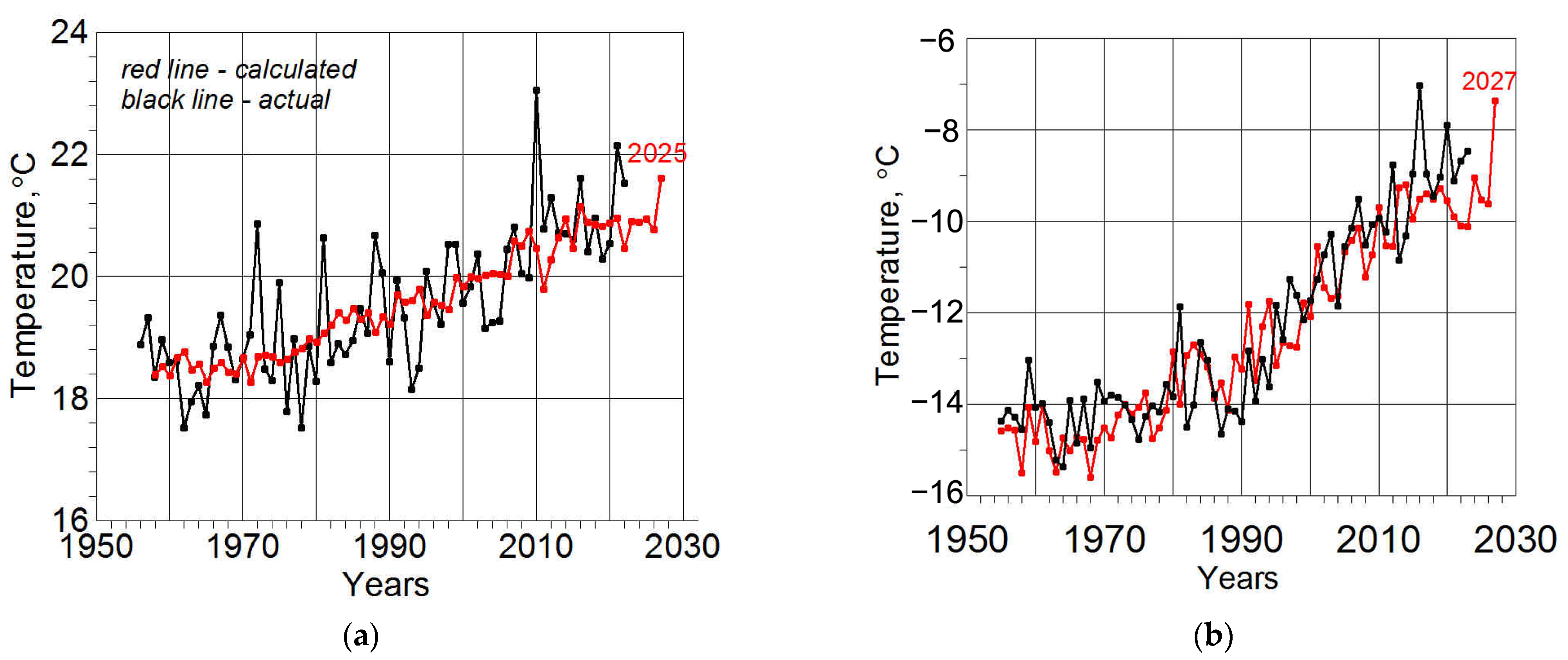
Experimental forecasts by regression models from Table 3 show an increase in SAT in both the Arctic and Eastern Europe over the next 3–4 years (see Figure 9). The SAT increase is due to the SST anomaly in the tropical North Atlantic, reflected by the “TNA” anomaly (more than three standard deviations from the mean) in the autumn of 2023, and a gradual increase in SST in the entire tropical region, reflected by an increase in the SL in Manila.

4. Discussion

The strong correlation between ocean characteristics (SST and SL) in the tropics and SAT in mid- and high latitudes, in addition to its obvious statistical significance, requires an indication of its causes. The first reason is the clear trends in the compared series of mid- and high-latitude SAT, low-latitude SST and SL. The greatest contribution from trends will occur when the SST and SL trend coefficients are equal to or greater than the SAT trend coefficients. However, the correlation between trends has no time lag, but between departures from trends such a lag appears, although the correlation coefficients between departures are significantly lower than between series with trends.
Removing trends from both predictors (SST and SL) and the predictant ( T E E or T A ) reduces the multiple regression coefficient for the average SAT in the Eastern European region to 0.20, and for the average SAT in the Arctic to 0.52. It should be emphasized that in both cases there is no correlation between deviations from the SL and SAT trends. However, the correlation between deviations from the “TNA” and SAT trends remains at the same time lag. The reason for this difference is explained by the small contribution (5%) of deviations from the trend to the variance of the SL series. In the meantime, contributions of deviations from trends to the variances in the T N A , T A and T E E series are 66, 45 and 35%, respectively. Thus, when comparing climate time series, it is desirable to keep their trends, which provide insight into how quickly the climate system is changing. Accounting for deviations from the trend in climate series ensures the identification of lags between processes whose mechanisms are associated with ocean–atmosphere interactions. Figure 10 illustrates the time-lag formation process considering the ocean–atmosphere interactions.
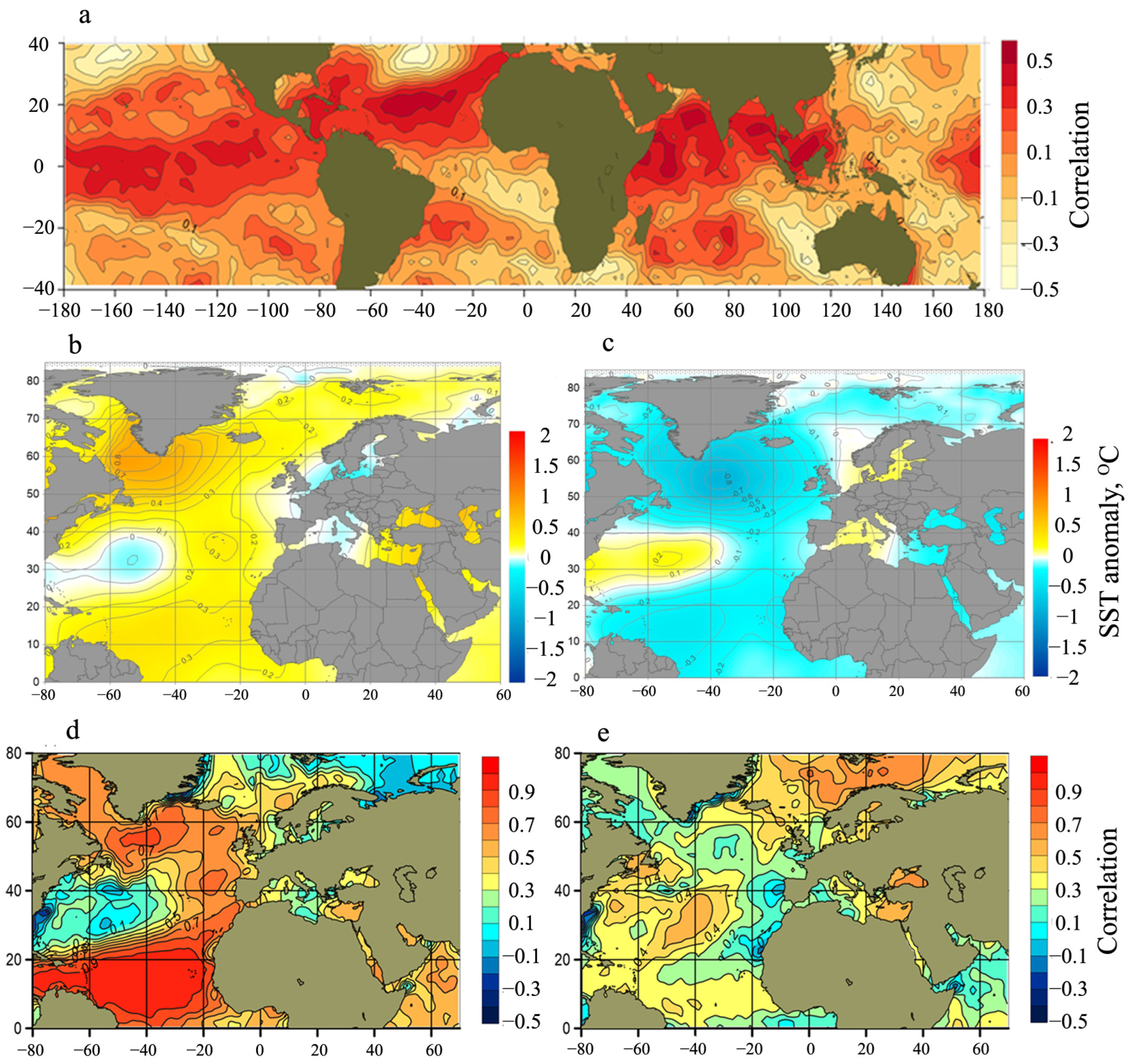
Let us provide some explanations for Figure 10. The lagged remote influence of tropical North Atlantic SST anomalies on Arctic air temperature anomalies (and sea ice) is related to the interaction between atmospheric and oceanic circulation patterns that transport heat from low to high latitudes [15,25,26]. In the atmosphere, such structures are the Hadley and Ferrel circulation cells, which are strengthened by positive SST anomalies in the tropics (Figure 10a), and the North Atlantic Oscillation (NAO), which is negatively correlated with SST anomalies in the tropics of the North Atlantic (Figure 10b,c). A positive SST anomaly corresponds to a negative NAO index and a positive SST anomaly north of 40° N, which manifests itself in the Norwegian and Barents Seas three years later (Figure 10d,e) and affects air temperature and sea ice in the Arctic.
It should be emphasized that the regression equations shown in Table 3 have an illustrative purpose, namely, to demonstrate the possibility of predictive use of the established relations; therefore, a validation procedure was not carried out. When developing forecasts, such validations will be required. In addition, the equations for the forecast can be updated when new data are received, i.e., we can use the “dynamic” method, which does not require the stability of the equations to be checked.

5. Conclusions

Low-frequency variability of tropical SST is reflected in changes in sea level, triggers the long-term component of atmospheric variability, and can become, together with sea level, a source of its predictability in high and mid-latitudes. Ocean heat transport from low to high latitudes, together with atmospheric circulation, is accompanied by a lag in the climate response in high latitudes relative to tropical SST anomalies by several years, providing a lead time for a possible forecast. Tropical SL data serve as indicators of the influence of low-latitude SST anomalies on air temperature in middle and especially high latitudes.
The relationship between ocean characteristics (SST and SL) and SAT can be used to construct data-driven (surrogate) models for predicting interannual changes in climate characteristics in middle and, especially, high latitudes.

Author Contributions

Conceptualization, G.A. and S.S.; methodology, G.A. and S.S.; software, N.G., N.K., Y.A. and M.S.; validation, G.A. and S.S.; formal analysis, G.A. and S.S.; data curation, N.G. and N.K.; writing—original draft preparation, G.A.; writing—review and editing, S.S.; visualization, N.G. and N.K.; supervision, G.A.; project administration, S.S.; funding acquisition, S.S. All authors have read and agreed to the published version of the manuscript.

Funding

This research was funded by RSF, grant number 23-47-10003.

Data Availability Statement

The data used in this study were retrieved from the following resources available in public domains: https://psl.noaa.gov, accessed on 5 June 2024; http://wdc.aari.ru/datasets, accessed on 7 June 2024; https://www.metoffice.gov.uk/hadobs/hadisst/, accessed on 12 June 2024.

Acknowledgments

The authors would like to thank the three anonymous reviewers for their time and valuable comments.

Conflicts of Interest

The authors declare no conflicts of interest.

Abbreviations

The following abbreviations and notations are used in this manuscript:
T E E ( t s ) Mean surface air temperature in the Eastern European region (45–60° N, 20–60° E) in summer
T A ( t a ) Mean surface air temperature in the Arctic in autumn
T N A Mean sea surface temperature anomaly in the Tropical North Atlantic (5.5–23.5° N, 15–57.5° N);
H M Mean sea level at Manila South Harbour (14.5° N, 120.97° E) in autumn
t Time (in years)
t s Summer season
t a Autumn season
RMultiple regression coefficient
A (%)Forecast accuracy on the dependent sample with an acceptable error of 0.674 standard deviation of the predictor
E (%)Forecast efficiency on the dependent sample
β 0 Detrended multiple regression coefficient (trends removed from predictors and predictant)

References

  1. Lorenz, E.N. The Nature and Theory of the General Circulation of the Atmosphere; World Meteorological Organization: Geneva, Switzerland, 1967; 161p. [Google Scholar]
  2. Golitsyn, G.S. A similarity approach to the general circulation of planetary atmospheres. Icarus 1970, 13, 1–24. [Google Scholar] [CrossRef]
  3. Hartmann, D.L. Global Physical Climatology; Academic Press: San Diego, CA, USA, 1994; 411p. [Google Scholar]
  4. Dymnikov, V.P.; Filatov, A.N. Mathematics of Climate Modeling; Birkhauser: Boston, MA, USA, 1997; 264p. [Google Scholar]
  5. Randall, D. An Introduction to the Global Circulation of the Atmosphere; Princeton University Press: Cambridge, MA, USA, 2015; 456p. [Google Scholar]
  6. Gulev, S.K.; Latif, M.; Keenlyside, N.; Park, W.; Koltermann, K.P. North Atlantic Ocean control on surface heat flux on multidecadal timescales. Nature 2013, 499, 464–467. [Google Scholar] [CrossRef] [PubMed]
  7. Schmitt, R.W. The ocean’s role in climate. Oceanography 2018, 31, 32–40. [Google Scholar] [CrossRef]
  8. Polonsky, A. The Ocean’s Role in Climate Change; Cambridge Scholars Publishing: Cambridge, UK, 2019; 294p. [Google Scholar]
  9. Williams, R.G.; Ceppi, P.; Roussenov, V.; Katavouta, A.; Meijers, A.J. The role of the Southern Ocean in the global climate response to carbon emissions. Phil. Trans. R. Soc. A 2023, 381, 20220062. [Google Scholar] [CrossRef]
  10. Ruprich-Robert, Y.; Moreno-Chamarro, E.; Levine, X.; Bellucci, A.; Cassou, C.; Castruccio, F.; Davini, P.; Eade, R.; Gastineau, G.; Hermanson, L.; et al. Impacts of Atlantic multidecadal variability on the tropical Pacific: A multi-model study. npj Clim. Atmos. Sci. 2021, 4, 33. [Google Scholar] [CrossRef]
  11. Årthun, M.; Eldevik, T.; Viste, E.; Drange, H.; Furevik, T.; Johnson, H.L.; Keenlyside, N.S. Skillful prediction of northern climate provided by the ocean. Nat. Commun. 2017, 8, 15875. [Google Scholar] [CrossRef] [PubMed]
  12. Smith, D.M.; Eade, R.; Scaife, A.A.; Caron, L.-P.; Danabasoglu, G.; DelSole, T.M.; Delworth, T.; Doblas-Reyes, F.J.; Dunstone, N.J.; Hermanson, L.; et al. Robust skill of decadal climate predictions. npj Clim. Atmos. Sci. 2019, 2, 13. [Google Scholar] [CrossRef]
  13. Hoerling, M.P.; Hurrell, J.W.; Xu, T. Tropical origins for recent North Atlantic climate change. Science 2001, 292, 90–92. [Google Scholar] [CrossRef]
  14. Årthun, M.; Eldevik, T. On anomalous ocean heat transport toward the Arctic and associated climate predictability. J. Clim. 2016, 29, 689–704. [Google Scholar] [CrossRef]
  15. Alekseev, G.V.; Glok, N.I.; Vyazilova, A.E.; Kharlanenkova, N.E.; Kulakov, M.Y. Influence of SST in low latitudes on the Arctic Warming and sea ice. J. Mar. Sci. Eng. 2021, 9, 1145. [Google Scholar] [CrossRef]
  16. Wettstein, J.J.; Deser, C. Internal variability in projections of twenty-first-century Arctic sea ice loss: Role of the large-scale atmospheric circulation. J. Clim. 2014, 27, 527–550. [Google Scholar] [CrossRef]
  17. Ye, K.; Wu, R.; Liu, Y. Interdecadal change of Eurasian snow, surface temperature, and atmospheric circulation in the late 1980s. J. Geophys. Res. Atmos. 2015, 120, 2738–2753. [Google Scholar] [CrossRef]
  18. Ding, Q.; Wallace, J.M.; Battisti, D.S.; Steig, E.J.; Gallant, A.J.E.; Kim, H.-J.; Geng, L. Tropical forcing of the recent rapid Arctic warming in northeastern Canada and Greenland. Nature 2014, 509, 209–212. [Google Scholar] [CrossRef] [PubMed]
  19. Goss, M.; Feldstein, S.B.; Lee, S. Stationary wave interface and its relation to tropical convection and Arctic warming. J. Clim. 2016, 16, 1369–1389. [Google Scholar] [CrossRef]
  20. Yoo, C.; Feldstein, S.B.; Lee, S. The impact of Madden-Julian Oscillation trend on the Arctic amplification ofsurface air temperature during 1979–2008 boreal winter. Geopjys. Res. Lett. 2011, 3, L24804. [Google Scholar]
  21. Yoo, C.; Lee, S.; Feldstein, S.B. Arctic response to an MJO-like tropical heating in an idealized GCM. J. Atmos. Sci. 2012, 69, 2379–2393. [Google Scholar] [CrossRef]
  22. Hou, Y.; Johnson, N.C.; Chang, C.; Sun, W.; Man, K.; Miao, Y.; Li, X. Cold Springs Over Mid-Latitude North America Induced by Tropical Atlantic Warming. Geophys. Res. Lett. 2023, 50, e2023GL104180. [Google Scholar] [CrossRef]
  23. Meehl, G.A.; Chung, C.T.Y.; Arblaster, J.M.; Holland, M.M.; Bitz, C.M. Tropical decadal variability and the rate of Arctic sea ice decrease. Geopjys. Res. Lett. 2018, 45, 11326–11333. [Google Scholar] [CrossRef]
  24. Yu, L.; Zhong, S.; Vihma, T.; Ding, S.; Sui, C.; Sun, B. The IPWP as a capacitor for autumn sea ice loss in Northeastern Canada. npj Clim. Atmos. Sci. 2024, 7, 259. [Google Scholar] [CrossRef]
  25. Alekseev, G.V.; Vyazilova, A.E.; Glok, N.I.; Ivanov, N.E.; Kharlanenkova, N.E. The effect of water temperature anomalies at low latitudes of the ocean on Arctic climate variations and their predictability. Arct. Ecol. Econ. 2019, 3, 73–83. [Google Scholar] [CrossRef]
  26. Alekseev, G.; Kuzmina, S.; Bobylev, L.; Urazgildeeva, A.; Gnatiuk, N. Impact of atmospheric heat and moisture transport on the Arctic warming. Int. J. Climatol. 2019, 39, 3582–3592. [Google Scholar] [CrossRef]
  27. Nesterov, E.S. North Atlantic Oscillation: Atmosphere and Ocean; Hydrometcenter Publishing: Moscow, Russia, 2013; 144p. [Google Scholar]
  28. Semenov, V.A.; Shelekhova, E.A.; Mokhov, I.I.; Zuev, V.V.; Koltermann, K.P. The influence of the Atlantic long-period oscillation on the formation of anomalous climatic regimes in the regions of northern Eurasia according to model calculations. Proc. Acad. Sci. 2014, 459, 742–745. [Google Scholar]
  29. De Deckker, P. The Indo-Pacific Waem Pool: Critical to world oceanography and world climate. Geosci. Lett. 2016, 3, 20. [Google Scholar] [CrossRef]
  30. Nesterov, E.S. Variability of atmospheric and ocean characteristics in the Atlantic-European region during El Niño and La Niña events. Meteorol. Hydrol. 2000, 8, 74–83. [Google Scholar]
  31. Mokhov, I.I.; Smirnov, D.A. Study of the mutual influence of the El Niño-Southern Oscillation and the North Atlantic and Arctic Oscillations. Proc. Acad. Sci. 2006, 42, 650–667. [Google Scholar] [CrossRef]
  32. Masson-Delmotte, V.; Zhai, P.; Pirani, A.; Connors, S.L.; Péan, C.; Berger, S.; Caud, N.; Chen, Y.; Goldfarb, L.; Gomis, M.I.; et al. (Eds.) IPCC, 2021: Climate Change 2021: The Physical Science Basis. In Contribution of Working Group I to the Sixth Assessment Report of the Intergovernmental Panel on Climate Change; Cambridge University Press: Cambridge, UK; New York, NY, USA, 2021; 2391p. [Google Scholar]
  33. Malinin, V.N.; Smirnov, M.A. Variability of the sea level in the tropical zone of the Pacific Ocean and El Niño-Southern Oscillation. Hydrometeorol. Ecol. 2022, 68, 463–477. [Google Scholar]
  34. Kalnay, E.; Kanamitsu, M.; Kistler, R.; Collins, W.; Deaven, D.; Gandin, L.; Iredell, M.; Saha, S.; White, G.; Woollen, J.; et al. The NCEP/NCAR 40-year reanalysis project. Bull. Amer. Meteor. Soc. 1996, 77, 437–471. [Google Scholar] [CrossRef]
  35. The NCEP/NCAR Reanalysis Project at the NOAA Physical Sciences Laboratory. Available online: https://psl.noaa.gov/data/reanalysis/reanalysis.shtml (accessed on 20 January 2021).
  36. Dee, D.P.; Uppala, S.M.; Simmons, A.J.; Berrisford, P.; Poli, P.; Kobayashi, S.; Andrae, U.; Balmaseda, M.A.; Balsamo, G.; Bauer, P.; et al. The ERA-Interim reanalysis: Configuration and performance of the data assimilation system. Q. J. R. Meteorol. Soc. 2011, 137, 553–597. [Google Scholar] [CrossRef]
  37. ECMWF Reanalysis—Interim (ERA—Interim). Available online: https://www.ecmwf.int/en/forecasts/dataset/ecmwf-reanalysis-interim (accessed on 21 January 2021).
  38. Hadley Centre Sea Ice and Sea Surface Temperature Data Set (HadISST). Available online: https://www.metoffice.gov.uk/hadobs/hadisst (accessed on 21 January 2021).
  39. Permanent Service for Mean Sea Level (PSMSL) Data. Available online: https://psmsl.org/data/ (accessed on 20 February 2024).
  40. All-Russian Research Institute of Hydrometeorological Information—World Data Centre. Available online: http://meteo.ru/data/ (accessed on 10 February 2024).
  41. Enfield, D.B.; Mestas-Nuñez, A.M.; Mayer, D.A.; Cid-Serrano, L. How ubiquitous is the dipole relationship in tropical Atlantic sea surface temperatures. J. Geophys. Res. Ocean 1999, 104, 7841–7848. [Google Scholar] [CrossRef]
Figure 1. Zero-year lagged correlation coefficients between autumn SST anomalies and seasonal SAT anomalies averaged over the Eastern European region: (a) summer; (b) autumn.
Climate 13 00084 g001
Figure 2. One-year lagged correlation coefficients between autumn SST anomalies and seasonal SAT anomalies averaged over the Eastern European region: (a) summer; (b) autumn.
Climate 13 00084 g002
Figure 3. Two-year lagged correlation coefficients between autumn SST anomalies and seasonal SAT anomalies averaged over the Eastern European region (45–60° N, 20–60° E): (a) summer; (b) autumn.
Climate 13 00084 g003
Figure 4. Three-year lagged correlation coefficients between autumn SST anomalies and seasonal SAT anomalies averaged over the Eastern European region: (a) summer; (b) autumn.
Climate 13 00084 g004
Figure 5. Zero-year lagged correlation coefficients between autumn SST anomalies and seasonal SAT anomalies averaged over the Arctic (70–87.5° N): (a) summer; (b) autumn.
Climate 13 00084 g005
Figure 6. Three-year lagged correlation coefficients between autumn SST anomalies and seasonal SAT anomalies averaged over the Arctic (70–87.5° N): (a) summer; (b) autumn.
Climate 13 00084 g006
Figure 7. Four-year lagged correlation coefficients between autumn SST anomalies and seasonal SAT anomalies averaged over the Arctic (70–87.5° N): (a) summer; (b) autumn.
Climate 13 00084 g007
Figure 8. Examples of cross-correlation coefficients calculated using ERA5 surface air temperature: (a) between T N A and T E E ; (b) between T N A and T A ; (c) between T N A and T E A . Solid lines (1) show correlation coefficients calculated with trends in time series, and dashed lines (2) illustrate correlation coefficients for detrended time series.
Climate 13 00084 g008
Figure 9. Predicted and actual SAT: (a) in Eastern Europe in summer; (b) in the Arctic in autumn.
Climate 13 00084 g009
Figure 10. Time-lag formation mechanism: (a) Correlation between October SST in the 40° S–40° N region of the Pacific, Indian and Atlantic Oceans and the 27-month-lag atmospheric sensible heat transport to the Arctic in winter via the Atlantic Gate at 70° N between 0 and 80° E. (b) Average annual SST anomalies for negative NAO index phase. (c) Average annual SST anomalies for positive NAO index phase. (d) Synchronous correlation between average annual SST in the tropical North Atlantic and average annual SST in the entire water area. (e) Three-year-lag correlation between average annual SST in the tropical North Atlantic and average annual SST in the entire water area.
Climate 13 00084 g010
Table 1. Lagged correlations between ocean characteristics (tropical SST and SL) and SAT in the Arctic and mid-latitudes calculated using NCEP reanalysis data. Time lags (in years) are shown in parentheses.
Sea Level AnomalyAverage Seasonal Surface Air TemperatureData Source
45–60° N, 20–60° E,
Eastern Europe
70–90° N
Arctic
70–90° N, 120–180° E
Eastern Arctic
“TNA”, autumn0.56 (+2) summer0.74 (+4) autumn0.66 (+3) autumnHadlSST, NCEP
1950–2023
Key West SL, autumn0.60 (+3) summer0.77 (+4) autumn0.77 (+3) autumnPMSL, NCEP
1950–2023
Manila sea level, autumn0.72 (+6) summer0.84 (+6) autumn0.81 (+5) autumnPMSL, NCEP
1950–2023
Table 2. Lagged correlations between ocean characteristics (tropical SST and SL) and SAT in the Arctic and mid-latitudes calculated using ERA5 reanalysis data. Time lags (in years) are shown in parentheses.
Sea Level AnomalyAverage Seasonal Surface Air TemperatureData Source
45–60° N, 20–60° E,
Eastern Europe
70–90° N
Arctic
70–90° N, 120–180° E
Eastern Arctic
“TNA”, autumn0.60 (+2) summer0.74 (+4) autumn0.72 (+3) autumnHadlSST, ERA5
1950–2023
Key West SL, autumn0.54 (+3) summer0.79 (+4) autumn0.73 (+3) autumnPMSL, ERA5
1950–2023
Manila sea level, autumn0.83 (+6) summer0.83 (+6) autumn0.77 (+5) autumnPMSL, ERA5
1950–2023
Table 3. Regression equations and estimates of the experimental forecast calculations based on data for 1950–2023.
Regression EquationsCharacteristics
RA (%)E (%) β 0
T E E t s = 0.60364 T N A t a 2 + 0.002643 H M t s 6 0.436333 0.7476310.20
T A t a = 2.2544 T N A t a 4 + 0.0050 H M t a 5 49.0147 0.9198280.52
Note: The notations used are shown in the Abbreviations and Notations section.
Disclaimer/Publisher’s Note: The statements, opinions and data contained in all publications are solely those of the individual author(s) and contributor(s) and not of MDPI and/or the editor(s). MDPI and/or the editor(s) disclaim responsibility for any injury to people or property resulting from any ideas, methods, instructions or products referred to in the content.