
Three-Century Climatology of Cold and Warm Spells and Snowfall Events in Padua, Italy (1725–2024)


Abstract
1. Introduction
2. Materials and Methods
2.1. Datasets
2.2. Methodology
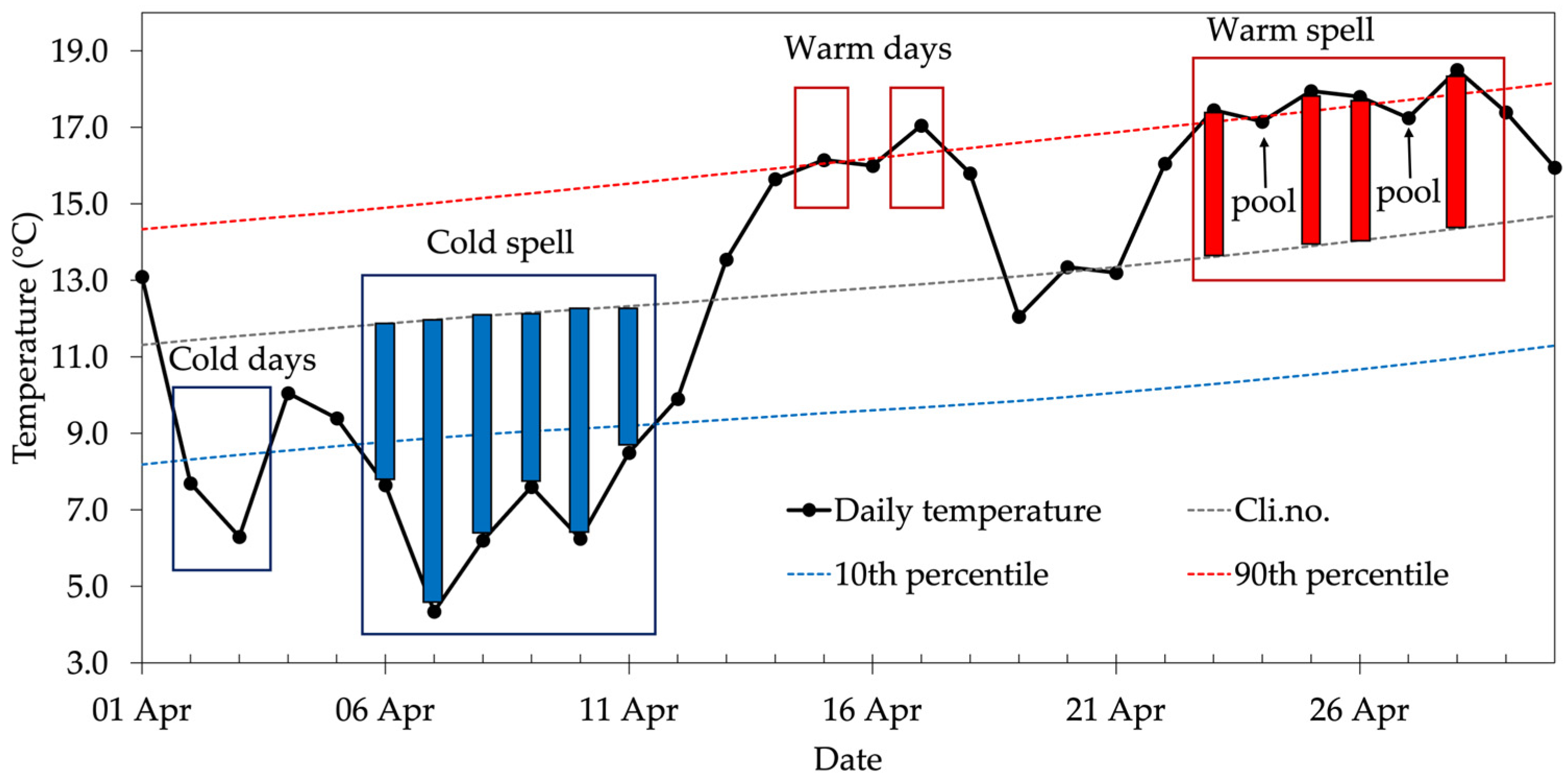
2.2.1. Cold and Warm Spells Characterization
2.2.2. Snow-Related Synoptic Situations
3. Results and Discussion
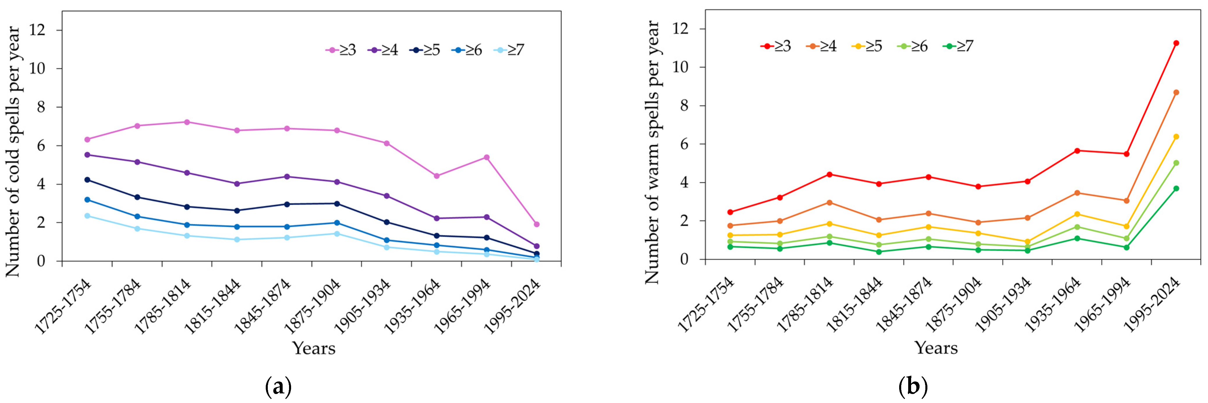
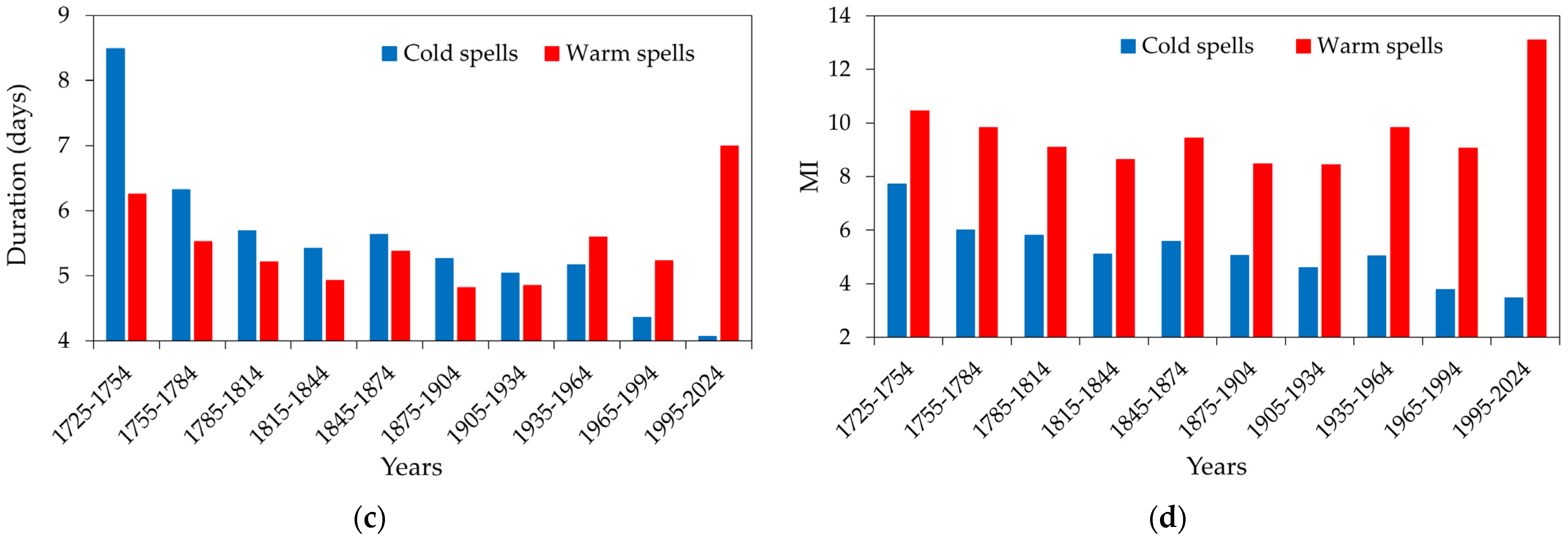
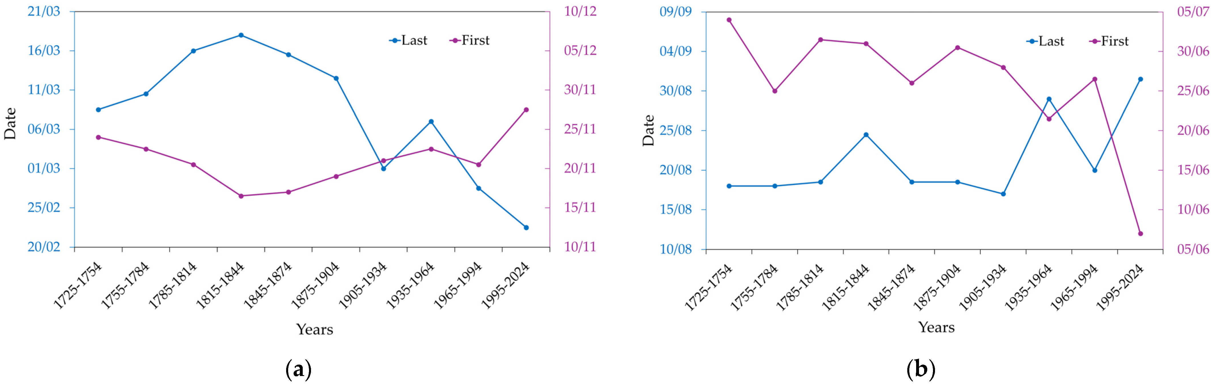
3.1. Cold and Warm Spells
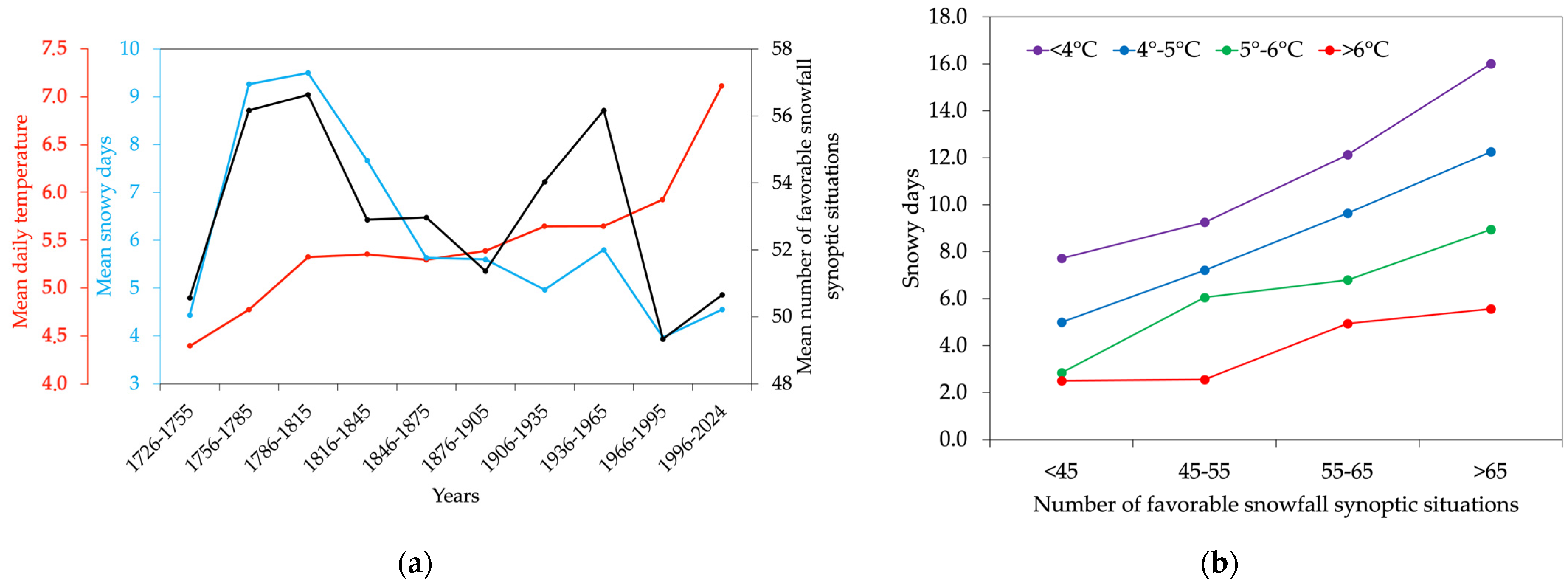
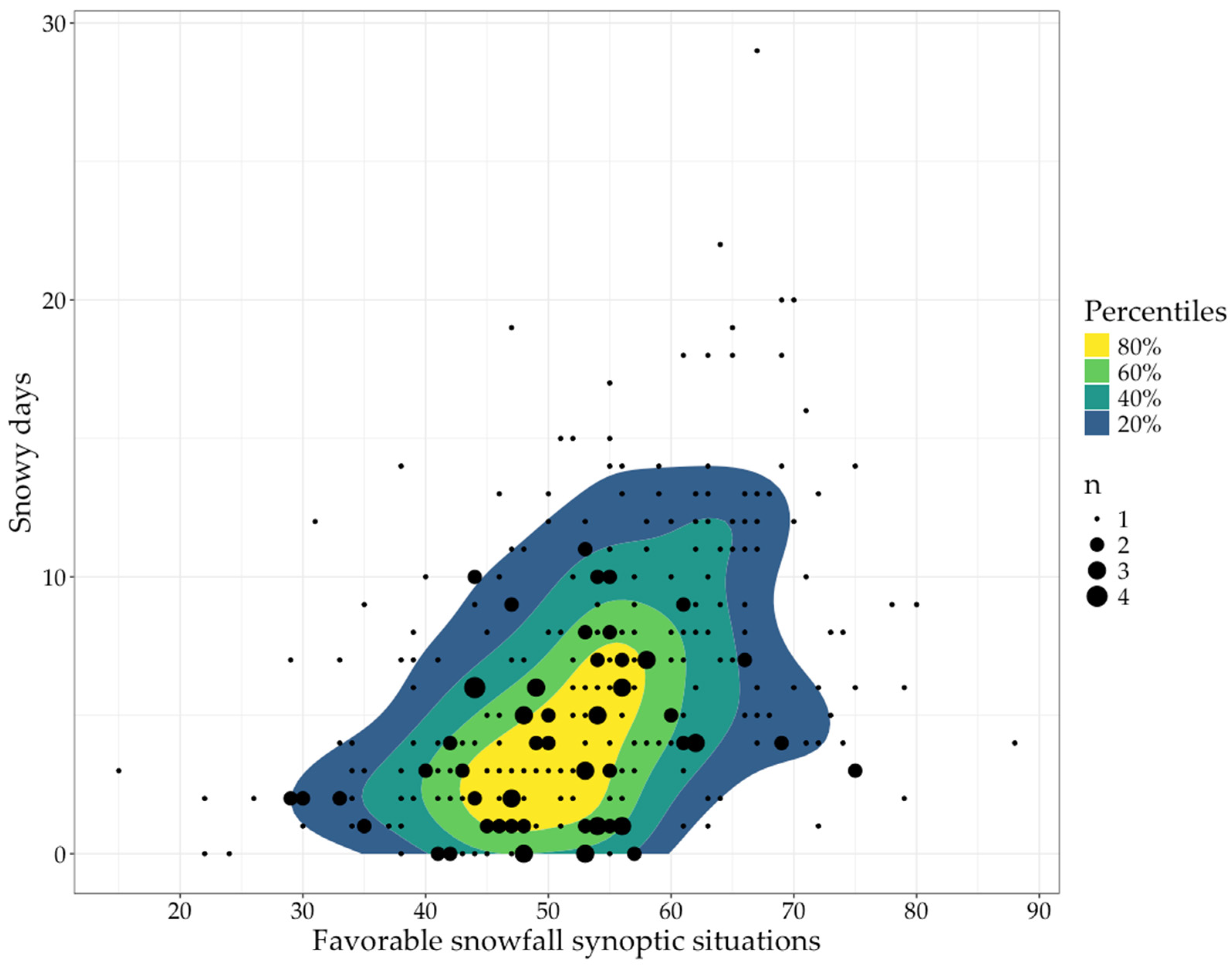
3.2. Snowfall
4. Conclusions
Supplementary Materials
Author Contributions
Funding
Data Availability Statement
Conflicts of Interest
References
- Camuffo, D. History of the Long Series of Daily Air Temperature in Padova (1725–1998). Clim. Change 2002, 53, 7–75. [Google Scholar] [CrossRef]
- Stefanini, C.; Becherini, F.; della Valle, A.; Camuffo, D. Homogenization of the Long Instrumental Daily-Temperature Series in Padua, Italy (1725–2023). Climate 2024, 12, 86. [Google Scholar] [CrossRef]
- Añel, J.; Fernández-González, M.; Labandeira, X.; López-Otero, X.; de la Torre, L. Impact of Cold Waves and Heat Waves on the Energy Production Sector. Atmosphere 2017, 8, 209. [Google Scholar] [CrossRef]
- Buras, A.; Rammig, A.; Zang, C.S. Quantifying impacts of the 2018 drought on European ecosystems in comparison to 2003. Biogeosciences 2020, 17, 1655–1672. [Google Scholar] [CrossRef]
- von Buttlar, J.; Zscheischler, J.; Rammig, A.; Sippel, S.; Reichstein, M.; Knohl, A.; Jung, M.; Menzer, O.; Arain, M.A.; Buchmann, N.; et al. Impacts of droughts and extreme-temperature events on gross primary production and ecosystem respiration: A systematic assessment across ecosystems and climate zones. Biogeosciences 2018, 15, 1293–1318. [Google Scholar] [CrossRef]
- Chapman, S.C.; Murphy, E.J.; Stainforth, D.A.; Watkins, N.W. Trends in Winter Warm Spells in the Central England Temperature Record. J. Appl. Meteorol. Clim. 2020, 59, 1069–1076. [Google Scholar] [CrossRef]
- Leporati, E.; Mercalli, L. Snowfall series of Turin, 1784–1992: Climatological analysis and action on structures. Ann. Glaciol. 1994, 19, 77–84. [Google Scholar] [CrossRef]
- Enzi, S.; Bertolin, C.; Diodato, N. Snowfall time-series reconstruction in Italy over the last 300 years. Holocene 2014, 24, 346–356. [Google Scholar] [CrossRef]
- Diodato, N.; Bertolin, C.; Bellocchi, G. Multi-Decadal Variability in the Snow-Cover Reconstruction at Parma Observatory (Northern Italy, 1681–2018 CE). Front. Earth Sci. 2020, 8, 2296–6463. [Google Scholar] [CrossRef]
- Colombo, N.; Valt, M.; Romano, E.; Salerno, F.; Godone, D.; Cianfarra, P.; Freppaz, M.; Maugeri, M.; Guyennon, N. Long-term trend of snow water equivalent in the Italian Alps. Climate 2022, 614A, 128532. [Google Scholar] [CrossRef]
- Avanzi, F.; Gabellani, S.; Delogu, F.; Silvestro, F.; Pignone, F.; Bruno, G.; Pulvirenti, L.; Squicciarino, G.; Fiori, E.; Rossi, L.; et al. IT-SNOW: A snow reanalysis for Italy blending modeling, in situ data, and satellite observations (2010–2021). Earth Syst. Sci. Data 2023, 15, 639–660. [Google Scholar] [CrossRef]
- Camuffo, D.; Bertolin, C.; Craievich, A.; Granziero, R.; Enzi, S. When the Lagoon was frozen over in Venice from A.D. 604 to 2012: Evidence from written documentary sources, visual arts and instrumental readings. Méditerranée 2017, 128, 35–53. [Google Scholar] [CrossRef]
- Garzena, D.; Acquaotta, F.; Fratianni, S. Analysis of the long-time climate data series for Turin and assessment of the city’s urban heat island. Weather 2019, 74, 353–359. [Google Scholar] [CrossRef]
- D’Errico, M.; Pons, F.; Yiou, P.; Tao, S.; Nardini, C.; Lunkeit, F.; Faranda, D. Present and future synoptic circulation patterns associated with cold and snowy spells over Italy. Earth Syst. Dynam. 2022, 13, 961–992. [Google Scholar] [CrossRef]
- Morlot, M.; Russo, S.; Feyen, L.; Formetta, G. Trends in heat and cold wave risks for the Italian Trentino-Alto Adige region from 1980 to 2018. Nat. Hazards Earth Syst. Sci. 2023, 23, 2593–2606. [Google Scholar] [CrossRef]
- Costanzini, S.; Boccolari, M.; Vega Parra, S.; Despini, F.; Lombroso, L.; Teggi, S. A comparative analysis of temperature trends at Modena Geophysical Observatory and Mount Cimone Observatory, Italy. Int. J. Climatol. 2024, 44, 4741–4766. [Google Scholar] [CrossRef]
- Di Bernardino, A.; Iannarelli, A.M.; Casadio, S.; Siani, A.M. Winter warm spells over Italy: Spatial–temporal variation and large-scale atmospheric circulation. Int. J. Climatol. 2024, 44, 1262–1275. [Google Scholar] [CrossRef]
- Camuffo, D.; Bertolin, C. Recovery of the early period of long instrumental time series of air temperature in Padua, Italy (1716–2007). Phys. Chem. Earth Parts A/B/C 2012, 40–41, 23–31. [Google Scholar] [CrossRef]
- Camuffo, D.; della Valle, A.; Becherini, F.; Zanini, V. Three centuries of daily precipitation in Padua, Italy, 1713–2018: History, relocations, gaps, homogeneity and raw data. Clim. Change 2020, 162, 923–942. [Google Scholar] [CrossRef]
- della Valle, A.; Camuffo, D.; Becherini, F.; Zanini, V. Recovering, correcting, and reconstructing precipitation data affected by gaps and irregular readings: The Padua series from 1812 to 1864. Clim. Change 2023, 176, 9. [Google Scholar] [CrossRef]
- Becherini, F.; Stefanini, C.; della Valle, A.; Rech, F.; Zecchini, F.; Camuffo, D. Multi-Secular Trend of Drought Indices in Padua, Italy. Climate 2024, 12, 218. [Google Scholar] [CrossRef]
- Camuffo, D.; Cocheo, C.; Sturaro, G. Corrections of Systematic Errors, Data Homogenisation and Climatic Analysis of the Padova Pressure Series (1725–1999). Clim. Change 2006, 76, 493–514. [Google Scholar] [CrossRef]
- Valler, V.; Franke, J.; Brugnara, Y.; Samakinwa, E.; Hand, R.; Lundstad, E.; Burgdorf, A.M.; Lipfert, L.; Friedman, A.R.; Brönnimann, S. ModE-RA: A global monthly paleo-reanalysis of the modern era 1421 to 2008. Sci. Data 2024, 11, 36. [Google Scholar] [CrossRef] [PubMed]
- EURO-CORDEX. Available online: https://www.euro-cordex.net/index.php.en (accessed on 31 January 2024).
- McCalla, R.J.; Day, E.E.D.; Millward, H.A. The relative concept of warm and cold spells of temperature: Methodology and application. Arch. Met. Geoph. Biokl. B 1978, 25, 323–336. [Google Scholar] [CrossRef]
- Ryti, N.R.I.; Guo, Y.; Jaakkola, J.J.K. Global Association of Cold Spells and Adverse Health Effects: A Systematic Review and Meta-Analysis. Environ. Health Perspect. 2016, 124, 12–22. [Google Scholar] [CrossRef]
- Lavaysse, C.; Cammalleri, C.; Dosio, A.; van der Schrier, G.; Toreti, A.; Vogt, J. Towards a monitoring system of temperature extremes in Europe. Nat. Hazards Earth Syst. Sci. 2018, 18, 91–104. [Google Scholar] [CrossRef]
- Efthymiadis, D.; Goodess, C.M.; Jones, P.D. Trends in Mediterranean gridded temperature extremes and large-scale circulation influences. Nat. Hazards Earth Syst. Sci. 2011, 11, 2199–2214. [Google Scholar] [CrossRef]
- Della Marta, P.M.; Haylock, M.R.; Luterbacher, J.; Wanner, H. Doubled length of western European summer heat waves since 1880. J. Geophys. Res. 2007, 112, D15103. [Google Scholar] [CrossRef]
- Sulikowska, A.; Wypych, A.E.M. Summer temperature extremes in Europe: How does the definition affect the results? Theor. Appl. Climatol. 2020, 141, 19–30. [Google Scholar] [CrossRef]
- Fischer, E.M.; Schär, C. Consistent geographical patterns of changes in high-impact European heatwaves. Nat. Geosci. 2010, 3, 398–403. [Google Scholar] [CrossRef]
- Perkins, S.E.; Alexander, L.V.; Nairn, J.R. Increasing frequency, inten- sity and duration of observed global heatwaves and warm spells. Geophys. Res. Lett. 2012, 39, L20714. [Google Scholar] [CrossRef]
- Stefanon, M.; Dandrea, F.; Drobinski, P. Heatwave classification over Europe and the Mediterranean region. Environ. Res. Lett. 2012, 7, 014023. [Google Scholar] [CrossRef]
- Russo, S.; Sillmann, J.; Fischer, E.M. Top ten European heatwaves since 1950 and their occurrence in the coming decades. Environ. Res. Lett. 2015, 10, 124003. [Google Scholar] [CrossRef]
- Mahlstein, I.; Spirig, C.; Liniger, M.A.; Appenzeller, C. Estimating daily climatologies for climate indices derived from climate model data and observations. J. Geophys. Res. Atmos. 2015, 120, 2808–2818. [Google Scholar] [CrossRef]
- loess: Local Polynomial Regression Fitting. Available online: https://www.rdocumentation.org/packages/stats/versions/3.6.2/topics/loess (accessed on 10 August 2024).
- wt: Wavelet Transformation, and a Simulation Algorithm. Available online: https://www.rdocumentation.org/packages/WaveletComp/versions/1.0/topics/wt (accessed on 16 June 2024).
- dplR: Dendrochronology Program Library in R. Available online: https://www.rdocumentation.org/packages/dplR/versions/1.7.6 (accessed on 16 June 2024).
- Ouellet, V.; Mingelbier, M.; Saint-Hilaire, A.; Morin, J. Frequency Analysis as a Tool for Assessing Adverse Conditions During a Massive Fish Kill in the St. Lawrence River, Canada. Water Qual. Res. J. Can. 2010, 45, 47–57. [Google Scholar] [CrossRef]
- Aksoy, H.; Cetin, M.; Eris, E.; Burgan, H.I.; Cavus, Y.; Yildirim, I.; Sivapalan, M. Critical drought intensity-duration-frequency curves based on total probability theorem-coupled frequency analysis. Hydrol. Sci. J. 2021, 66, 1337–1358. [Google Scholar] [CrossRef]
- Paris-London Westerly Index-Monthly & Daily SLP for Paris (Back to 1670) and London (Back to 1692). Available online: https://crudata.uea.ac.uk/cru/data/parislondon/ (accessed on 14 October 2024).
- Bergström, H.; Moberg, A. Daily Air Temperature and Pressure Series for Uppsala (1722–1998). In Improved Understanding of Past Climatic Variability from Early Daily European Instrumental Sources; Camuffo, D., Jones, P., Eds.; Springer: Dordrecht, The Netherlands, 2002; pp. 213–252. [Google Scholar] [CrossRef]
- European Climate Assessment & Dataset. Available online: https://www.ecad.eu/dailydata/ (accessed on 31 January 2025).
- kmeans: K-Means Clustering. Available online: https://www.rdocumentation.org/packages/stats/versions/3.6.2/topics/kmeans (accessed on 16 June 2024).
- Brönnimann, S.; Filipiak, J.; Chen, S.; Pfister, L. The weather of 1740, the coldest year in central Europe in 600 years. Clim. Past 2024, 20, 2219–2235. [Google Scholar] [CrossRef]
- Brugnara, Y.; Brönnimann, S. Revisiting the early instrumental temperature records of Basel and Geneva. Meteorol. Z. (Contrib. Atm. Sci.) 2023, 32, 513–527. [Google Scholar] [CrossRef]
- Camuffo, D.; della Valle, A.; Bertolin, C.; Santorelli, E. Temperature observations in Bologna, Italy, from 1715 to 1815: A comparison with other contemporary series and an overview of three centuries of changing climate. Clim. Change 2017, 142, 7–22. [Google Scholar] [CrossRef]
- Meehl, G.A.; Tebaldi, C.; Walton, G.; Easterling, D.; McDaniel, L. Relative increase of record high maximum temperatures compared to record low minimum temperatures in the U.S. Geophys. Res. Lett. 2009, 36, L23701. [Google Scholar] [CrossRef]
- Twardosz, R.; Łupikasza, E.; Niedźwiedź, T.; Walanus, A. Long-term variability of occurrence of precipitation forms in winter in Kraków, Poland. Clim. Change 2012, 113, 623–638. [Google Scholar] [CrossRef]
- kde2d: Two-Dimensional Kernel Density Estimation. Available online: https://www.rdocumentation.org/packages/MASS/versions/7.3-64/topics/kde2d (accessed on 1 February 2025).
- NOAA/CIRES/DOE 20th Century Reanalysis (V3). Available online: https://www.psl.noaa.gov/data/gridded/data.20thC_ReanV3.html (accessed on 16 June 2024).
- Casty, C.; Wanner, H.; Luterbacher, J.; Esper, J.; Böhm, R. Temperature and precipitation variability in the European Alps since 1500. Int. J. Climatol. 2005, 25, 1855–1880. [Google Scholar] [CrossRef]
- Valler, V.; Franke, J.; Brugnara, Y.; Brönnimann, S. An updated global atmospheric paleo-reanalysis covering the last 400 years. Geosci. Data J. 2022, 9, 89–107. [Google Scholar] [CrossRef] [PubMed]
- Reiter, L.R. Handbook for Forecasters in the Mediterranean; Environment Prediction Research Facility, Naval Postgraduate School: Monterey, CA, USA, 1975. [Google Scholar]
- Busato, F.; Lazzarin, R.M.; Noro, M. Three years of study of the Urban Heat Island in Padua: Experimental results. Sustain. Cities Soc. 2014, 10, 251–258. [Google Scholar] [CrossRef]
- Noro, M.; Busato, F.; Lazzarin, R.M. Urban heat island in Padua, Italy: Experimental and theoretical analysis. Indoor Built Environ. 2015, 24, 514–533. [Google Scholar] [CrossRef]
- Noro, M.; Lazzarin, R.M. Urban heat island in Padua, Italy: Simulation analysis and mitigation strategies. Urban Clim. 2015, 14, 187–196. [Google Scholar] [CrossRef]
- Noro, M.; Lazzarin, R.M.; Busato, F. The Urban Corridor of Venice and The Case of Padua. In Counteracting Urban Heat Island Effects in a Global Climate Change Scenario; Musco, F., Ed.; Springer: Cham, Switzerland, 2016; pp. 201–219. [Google Scholar] [CrossRef]
- Bertolin, C.; Camuffo, D. Urban Climate and Health: Two Strictly Connected Topics in the History of Meteorology. In Sustainability in Energy and Buildings. Smart Innovation, Systems and Technologies; Littlewood, J., Howlett, R., Capozzoli, A., Jain, L., Eds.; Springer: Singapore, 2020; Volume 163. [Google Scholar] [CrossRef]
- Todeschi, V.; Pappalardo, S.E.; Zanetti, C.; Peroni, F.; De Marchi, M. Climate Justice in the City: Mapping Heat-Related Risk for Climate Change Mitigation of the Urban and Peri-Urban Area of Padua (Italy). ISPRS Int. J. Geo-Inf. 2022, 11, 490. [Google Scholar] [CrossRef]
- Pappalardo, S.E.; Zanetti, C.; Todeschi, V. Mapping urban heat islands and heat-related risk during heat waves from a climate justice perspective: A case study in the municipality of Padua (Italy) for inclusive adaptation policies. Landsc. Urban Plan. 2023, 238, 104831. [Google Scholar] [CrossRef]


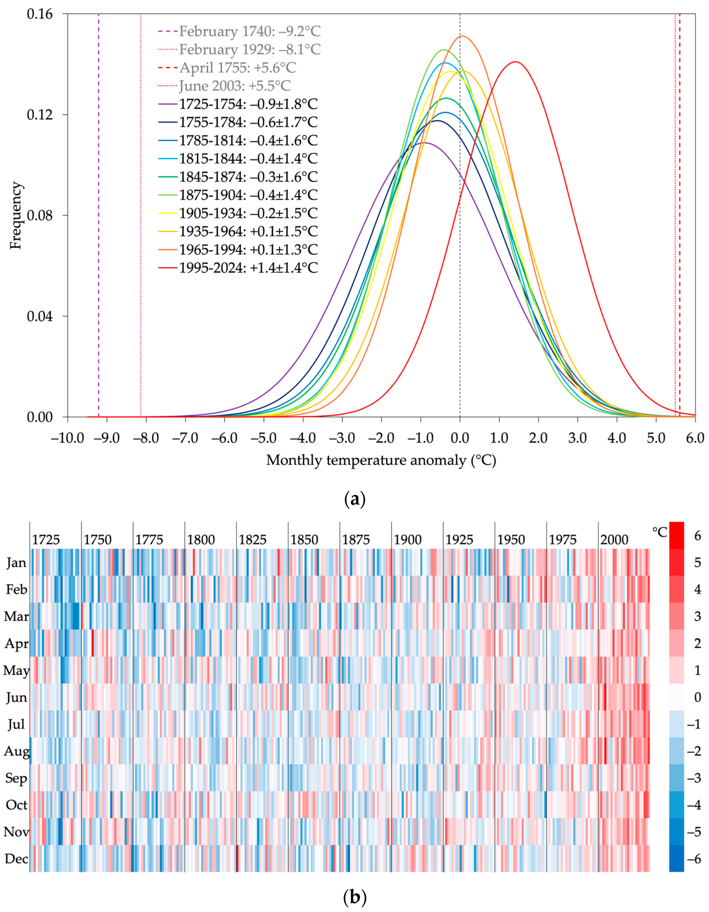
| Monthly Anomaly | 1725–1754 | 1965–1994 | 1995–2024 |
|---|---|---|---|
| <−2 °C | 23% | 4% | 0.5% |
| >+2 °C | 7% | 10% | 40% |
| Main Feature | Dates | Duration (Days) | Extreme Daily Anomaly (°C) | Extreme Daily Mean Value (°C) | ||
|---|---|---|---|---|---|---|
| Cold spells | Max duration | 14 February–5 April 1808 | 52 | −69.0 | −11.7° | −2.4° |
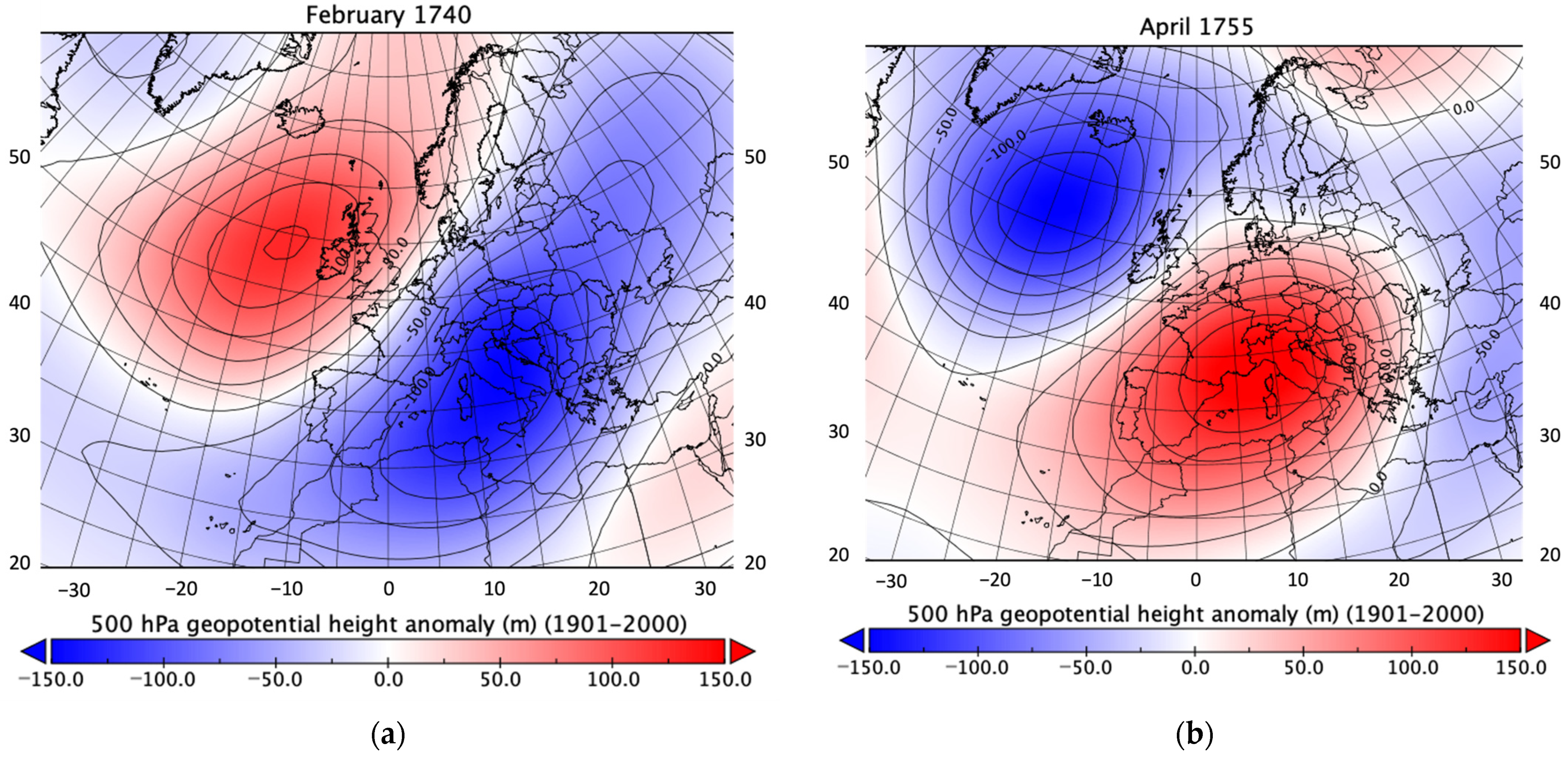
| Max intensity | 28 January–12 March 1740 | 44 | −78.1 | −12.8° | −8.4° | |
| Min daily anomaly | 28 January–26 February 1929 | 29 | −50.9 | −15.4° | −11.1° | |
| Min daily value | 12 December 1788–10 January 1789 | 28 | −50.4 | −14.0° | −11.2° | |
| Warm spells | Max duration Max intensity | 8 July–4 September 2024 | 55 | 112.3 | +7.5° | 30.4° |
| Max daily anomaly | 31 March–12 April 2011 | 13 | 29.7 | +10.7° | 22.9° | |
| Max daily value | 2–30 August 2003 | 27 | 63.0 | +8.4° | 32.1° |
Disclaimer/Publisher’s Note: The statements, opinions and data contained in all publications are solely those of the individual author(s) and contributor(s) and not of MDPI and/or the editor(s). MDPI and/or the editor(s) disclaim responsibility for any injury to people or property resulting from any ideas, methods, instructions or products referred to in the content. |
© 2025 by the authors. Licensee MDPI, Basel, Switzerland. This article is an open access article distributed under the terms and conditions of the Creative Commons Attribution (CC BY) license (https://creativecommons.org/licenses/by/4.0/).
Share and Cite
Stefanini, C.; Becherini, F.; della Valle, A.; Camuffo, D. Three-Century Climatology of Cold and Warm Spells and Snowfall Events in Padua, Italy (1725–2024). Climate 2025, 13, 70. https://doi.org/10.3390/cli13040070
Stefanini C, Becherini F, della Valle A, Camuffo D. Three-Century Climatology of Cold and Warm Spells and Snowfall Events in Padua, Italy (1725–2024). Climate. 2025; 13(4):70. https://doi.org/10.3390/cli13040070
Chicago/Turabian StyleStefanini, Claudio, Francesca Becherini, Antonio della Valle, and Dario Camuffo. 2025. "Three-Century Climatology of Cold and Warm Spells and Snowfall Events in Padua, Italy (1725–2024)" Climate 13, no. 4: 70. https://doi.org/10.3390/cli13040070
APA StyleStefanini, C., Becherini, F., della Valle, A., & Camuffo, D. (2025). Three-Century Climatology of Cold and Warm Spells and Snowfall Events in Padua, Italy (1725–2024). Climate, 13(4), 70. https://doi.org/10.3390/cli13040070