Abstract
The relocation of Indonesia’s capital to Nusantara in East Kalimantan has raised concerns about microclimatic impacts resulting from proposed land use and land cover (LULC) changes. This study explored strategies to mitigate these impacts by using dynamical downscaling with the Weather Research and Forecasting model integrated with the urban canopy model (WRF-UCM). Numerical experiments at a 1 km spatial resolution were used to evaluate the impacts of green and mitigation strategies on the proposed master plan. In this process, five scenarios were analyzed, incorporating varying proportions of blue–green spaces and modifications to building walls and roof albedos. Among them, scenario 5, with 65% blue–green spaces, exhibited the highest cooling potential, reducing average urban surface temperatures by approximately 2 °C. In contrast, scenario 4, which allocated equal shares of built-up areas and mixed forests (50% each), achieved a more modest reduction of approximately 1 °C. The adoption of nature-based solutions and sustainable urban planning in Nusantara underscores the feasibility of climate-resilient urban development. This framework could inspire other cities worldwide, showcasing how urban growth can align with environmental sustainability.
1. Introduction
Urbanization is a significant global phenomenon characterized by the increasing migration of populations from rural areas to urban areas, leading to the expansion of cities and towns [1]. This process is closely linked to changes in land use and land cover (LULC), which refer to the human activities that modify the landscape and the physical characteristics of the land surface, respectively. As urban areas expand, landscapes such as forests, wetlands, and agricultural lands are often converted into built environments, resulting in a marked increase in impervious surfaces such as roads and buildings. This transformation not only alters the physical appearance of the landscape but also alters the physical and biophysical characteristics of land surfaces, such as albedo, evapotranspiration, the sky view factor, soil moisture, heat capacity, etc., which can alter the surface energy balance and hence microclimate of the region [2].
In the past, several researchers have emphasized the effect of urbanization on the microclimate of a region by analyzing the associations between changes in LULC and microclimatic parameters such as temperature [3,4,5,6,7,8,9]. For example, in the case of Addis Ababa city, which is located in Ethiopia, Negesse et al. (2024) reported that over a span of 30 years, an increase of 39 km2 in the built-up area induced a 5.4 °C increase in temperature [10]. Uddin et al. (2022) reported that, from 2000 to 2017, 25.33% of the urban area in Dhaka city grew, increasing the temperature by approximately 3 °C [11]. Due to urbanization, a 1.2 °C increase in the average surface temperature of Kumasi, Ghana, was reported by [12]. In 2021, Hassan et al. (2021) studied the microclimatic effects of urbanization on South Asian cities between 2000 and 2019. During this period, vegetated areas were significantly reduced across all cities, whereas urban areas expanded considerably [13]. This land use change resulted in an increase in the mean land surface temperature in peri-urban regions, with an increase ranging from 1 to 2 °C. In addition, several studies have shown a positive correlation between city temperature and impervious surfaces [14,15,16,17]. Recently, a study in subtropical regions reported that, in Indian cities, a decrease of 1% in seasonal changes in vegetation vigor led to an increase in the seasonal intensity of urban heat islands by 1.74 °C [2]. These microclimatic changes induced by urbanization have significant impacts on several aspects, including human health [18], economic growth [19], the environment [20], greenhouse gas emissions [21], stormwater runoff [22], and mortality rates [23].
In the case of Indonesia, at present, the government is undertaking the enormous task of relocating its capital city from Jakarta to Nusantara, which is driven by various factors, such as Jakarta’s overpopulation, sinking land, and environmental degradation. During this relocation process, intensive urbanization is expected in Nusantara. This process of urbanization can drastically alter local weather patterns, leading to several detrimental consequences. One major concern is the increase in a region’s surface air temperature due to factors such as reduced vegetation, increased impervious surfaces (concrete and asphalt), and anthropogenic heat emissions from buildings and vehicles. This increased temperature can exacerbate heat stress, impacting public health and increasing energy consumption for cooling. Nusantara’s development provides a unique context to implement sustainable urban planning strategies from the outset, mitigating these negative impacts. Studying potential microclimate impacts allows proactive mitigation measures, such as incorporating green spaces, utilizing sustainable building materials, and implementing efficient transportation systems. While the specific geographical context of Nusantara is unique, the challenges of managing the impacts of urbanization on the microclimate are typical of large-scale development projects in tropical climates. In recent years, many climate-associated studies have been carried out by researchers. Most of these investigations have focused on hydrometeorological issues [24,25,26]. However, very few studies have investigated the thermal characteristics of the region. For example, a recent study [27] revealed that in a new capital region of Nusantara, a 4% increase in built-up areas is expected to increase the discomfort index by 0.1–0.2 °C. Another study over the Nusantara region [28] subsequently carried out satellite-based climatic quantification of surface urban heat islands. The results of their study revealed that in Nusantara, the intensity of surface urban heat islands is highest in September, October, and November, whereas the lowest intensity occurs in June, July, and August. Subsequently, numerical modeling [29] was used to simulate the impacts of expected urbanization on the surface air temperature of Nusantara. The results of this study reveal that land transformation from vegetation to urban areas can increase the mean surface air temperature of a region by 1.17 °C to 1.77 °C. Despite these studies, comprehensive analyses of (i) how different urban design strategies, such as the incorporation of green spaces, sustainable materials, and cooling technologies, can mitigate the rise in surface air temperature are lacking. (ii) Efficiency of different mitigation strategies.
In the past, several global attempts have been made to design and evaluate the efficiency of various mitigation strategies, including green, blue, and cooling material-based infrastructures, to minimize the impact of urbanization on the microclimate. For example, Sen et al. (2019) conducted an experiment in Phoenix City, Arizona, to replace all pavement surfaces with more reflective concrete pavements, which led to a decrease in air temperature of approximately 0.20–0.40 °C [30]. In the case of European urban areas, Marando et al. (2020) reported that at least 16% of the area of 601 cities (known as functional urban areas) needs to be covered by green infrastructure to achieve a 1 °C reduction in the average summer temperature [31]. However, most of the abovementioned mitigation studies have been carried out over functional urban agglomerations, which makes them difficult to implement on the ground for several reasons: (i) densely built areas leave little room for green spaces or water features, (ii) functional cities have aged infrastructure systems that are difficult to modify for the implementation of green solutions, and (iii) people in these areas may resist changes due to disruptions or the fear of losing property value. Thus, it is important to check the climate sensitivity of future development plans for cities before urban areas are developed and established.
Moreover, a limited number of studies have attempted to quantify the effect of proposed urbanization on the urban microclimate and test the efficiency of mitigation strategies by using the Weather Research and Forecasting model coupled with the urban canopy model (WRF-UCM). For example, Kubota et al. (2017) explored the impact of urbanization and land use changes on urban heat islands in Hanoi, Vietnam, with a focus on the effectiveness of green strategies in mitigating rising temperatures. This study compared the results of the master plan condition with those of other scenarios involving different green strategies to evaluate their cooling effects [32]. Vinayak et al. (2022) investigated the role of cool roofs/walls in minimizing the impact of future urbanization on temperature in Mumbai, India [33]. However, such studies emphasize the role of mitigation strategies in minimizing the microclimatic effect of urban development via the WRF-UCM. However, these studies fail to assess the combined effects of blue-green infrastructure and cooling material strategies, providing a complete understanding of mitigation potential compared with single-strategy evaluations.
Therefore, the present study aims to assess the effectiveness of integrated green–blue strategies combined with cool roof and wall techniques (soft solutions) for urban cooling in the development of Nusantara Capital City, Indonesia. The evaluation spans from predevelopment conditions to various urban-green configurations and uses the WRF-UCM. To the best of the author’s knowledge, this study represents a quantitative numerical approach that evaluates the efficiency of integrated mitigation approaches that are useful for proactive climate-sensitive urban planning rather than reactive mitigation in established cities.
2. Materials and Methods
2.1. Study Area
The present study was conducted over the capital city of Nusantara and surrounding regions in East Kalimantan Province, Indonesia. It spans from 116.25° E to 117.25° E and from 1.25° S to 0.30° S. The total area of the region is 561.81 km2, combining the government center core area (KIPP) and the main area of the Nusantara capital city (KIKN), while the entire remaining area (IKN) will be considered for future development, as shown in Figure 1. The elevation of the study area ranges from 0 to 200 m above sea level. The current population in this study area is approximately 1.7 million people, with projections suggesting that approximately 1.176 million new urban dwellers will be settled by 2035.
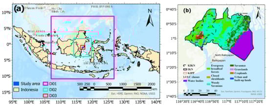
Figure 1.
Study area map representing (a) Indonesia and the domains for the Weather Research and Forecast (WRF) model and the location of the Nusantara capital city and (b) the location of the government center core area (KIPP), the main area of Nusantara (KIKN), and the entire area, including the Nusantara capital city future development plan (IKN) and the actual land use and land cover (LULC) classes across the Nusantara region.
The climate zone of the study area is classified as Zone 1A, the subequatorial climate zone [34]. This area primarily experiences two seasons: the dry season (July–October) and the wet season (November–June), both of which are strongly influenced by the El Niño Southern Oscillation (ENSO) and Indian Ocean Dipole (IOD) in the annual cycle [34]. The dry season was recorded as the hottest period, with October being the month when the surface air temperature reached 28.5 °C during the period from 2016 to 2020. In contrast, during the wet season, the maximum rainfall occurred in January and March (247 mm) over the past five years from 2016 to 2020 (Figure A1 [Appendix A]).
According to government plans, the capital will be relocated from Jakarta to Nusantara by 2024. A total of 25% of the total study area is expected to be transformed from natural surfaces into built-up areas, including commercial areas, industrial complexes, housing, and residential zones. However, during these transformations, the government aims to maintain 75% of the entire area as conserved green space. Specifically, in KIPP, 50% of the area is preserved as greenery. As mentioned in the previous section, this alteration may induce microclimatic changes by modifying terrestrial land surface properties. According to an official report from the government of Indonesia (Law of the Republic of Indonesia, number 3 of 2022 on National Capital), during the development of a new capital region, the greatest alteration in LULC will occur in the KIPP area, which will significantly modify microclimate conditions. Therefore, this study focuses on the KIPP region to assess the efficiency of the proposed mitigation strategies for urban cooling.
2.2. Masterplan of Nusantara Capital City
According to the recently published IKN law, the new capital city area is divided into a structured regional hierarchy: the KIPP covers 6671 ha, the IKN area covers 56,180 ha, and the IKN expansion area covers 199,962 ha. The total designated area for IKN is approximately 256,142 ha of land and 68,189 ha of water, extending into the sea from the coastline. The relocation of the capital city from Java is intended to shift national development from a Java-centric approach to an Indonesia-centric approach. The greenfield-developed city is based on three basic principles, i.e., the forest city, sponge city, and smart city, according to the master plan outlined in IKN law. The long-term development goal for IKNs is to achieve 75% green coverage of the entire area (Figure 1b). Moreover, the KIKN and KIPP (Figure 1b) areas are targeted to have 50% green coverage. This 50% green coverage within KIKN development consists of biodiversity corridors, urban forests, botanical gardens, green belts, green open spaces, and riparian parks.
2.3. Land Use and Land Cover Scenarios
According to the Collection 6 MODIS Land Cover MCD12Q1 (500 m spatial resolution) LULC dataset [35], the Nusantara region consists of eight classes, namely, water bodies, evergreen broadleaf forests, closed shrublands, woody savannas, savannas, grasslands, croplands, and urban built-up lands (see Table 1). The spatial distribution of LULC over Nusantara is dominated by woody savannas (43.49%) and evergreen broadleaf forests (24.21%), which cover 1642.75 km2 and 914.25 km2, respectively. In the development plan for the new capital city, the government aims to preserve biodiversity, natural resources, and “blue–green spaces” in the region by maintaining greenery in land use and land cover types. However, the proposed spatial development plan is not publicly available. Therefore, to quantify the effects of future urban development in Nusantara, this study proposed five hypothetical scenarios (Figure 2b–f).

Table 1.
Land use/land cover classification from Collection 6 MODIS Land Cover MCD12Q1 (500 m spatial resolution) [35].
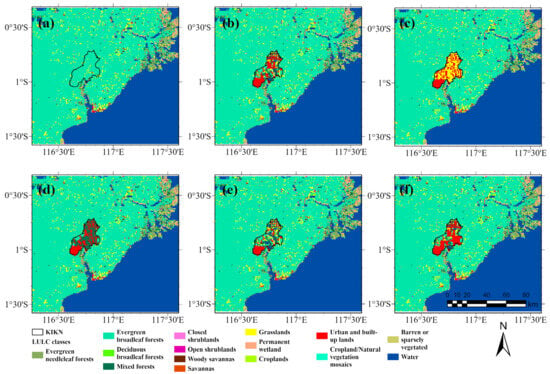
Figure 2.
Variations in the LULC data for the KIKN area used for the WRF numerical simulations: (a) scenario 1 (before development); (b) scenario 2, representing the baseline (50% greenery and 50% urban); (c) scenario 3 (50% grasslands and 50% urban); (d) scenario 4 (50% mixed forest and 50% urban); (e) scenario 5 (65% greenery and 35% urban); (f) scenario 6 (35% greenery and 65% urban).
The preparation of these scenarios is based on the provisions formulated in state law for the development of a safe, modern, sustainable, and resilient national capital city, which serves as a reference for developing and organizing other regions in Indonesia [36]. The hypotheses were developed using official source information, paying attention to the detailed proportion of blue and green infrastructure cover according to various uses. This includes ponds, biodiversity corridors, urban forests, botanical gardens, green belts, green open spaces, and riparian parks.
Indonesia’s new capital as a “forest city” embodies nature-based solutions (NBSs), harmonizing urban development with environmental preservation. This approach integrates biodiversity conservation, sustainable land use, and green infrastructure to create a model city addressing climate change and urbanization challenges. The plan aims to protect, manage, and restore forests to cover 65% of the city’s area, reducing emissions and enhancing resilience.
Therefore, in this study, two main scenarios were developed, viz. scenarios 1 (before development) and 5 (65% greenery and 35% urban areas) were used. Microclimatic simulations carried out with scenario 1 serve as a baseline scenario. On the other hand, scenario five is based on the urban development policy prepared by the Nusantara Development Authority. According to the chairperson of Technology Transformation and Innovation, Nusantara Authority, the IKN part of Nusantara city will be developed as a forest city, where 65% of the area is dedicated to tropical forest and 35% of the area is urban infrastructure, which has been replicated as scenario 5 [36].
Apart from these two scenarios, simulating the impacts of other hypothetical land use and land cover (LULC) scenarios, viz. scenario 2 (50% greenery and 50% urban); scenario 3 (50% grasslands and 50% urban); scenario 4 (50% mixed forest and 50% urban); and scenario 6 (35% greenery and 65% urban) is essential for a comprehensive assessment of future urbanization’s environmental and urban climate effects. For example, scenarios with different vegetation types, such as tropical forests, grasslands, and mixed forests, help identify which vegetation type is most effective in mitigating urban heat and enhancing ecosystem services. Scenarios such as 6 (35% greenery, 65% urban) simulate highly urbanized conditions, revealing critical thresholds beyond which urban expansion significantly degrades climatic conditions and ecosystem stability.
The comparative assessment of microclimatic simulations of different scenarios supports decision-making by providing statistical data on the trade-offs between urbanization and environmental sustainability. This study highlights the implications of specific development policies for urban climate and resilience.
2.4. WRF-UCM
Meteorological modeling and simulations were performed to assess key atmospheric parameters, including air temperature, relative humidity, surface wind patterns, and atmospheric pressure, via the Advanced Research Weather Research and Forecasting (ARW-WRF) model. The ARW-WRF model is a three-dimensional, nonhydrostatic mesoscale meteorological model developed by the National Centre for Atmospheric Research (NCAR). It utilizes a nonhydrostatic compressible framework for governing equations in spherical and sigma coordinates.
The WRF model integrates various physical processes, such as cumulus cloud dynamics, atmospheric microphysics, planetary boundary layer (PBL) processes, and radiation transfer, through diverse physics parameterizations. To evaluate the microclimatic impacts of future development in the Nusantara capital city area, the WRF model (version 4.6.0) coupled with the single-layer urban canopy model (UCM) was utilized. This coupling allows simulation of urban heat, momentum, and water vapor exchanges within a mesoscale framework.
Mesoscale models operate at spatial resolutions of a few kilometers, assuming homogeneous conditions within a given zone. Surface properties such as albedo, emissivity, and roughness are represented as bulk values, limiting the model’s ability to capture fine-scale interactions between buildings and their environments. While increasing the domain size and spatial resolution could address these limitations, it incurs significant computational costs. Despite these constraints, mesoscale models remain effective for analyzing large-scale regional climatic variations and evaluating urban-scale mitigation strategies, such as urban greening.
2.5. Numerical Experiment Setup
In this study, the model was executed for 21 days, from 10 October to 31 October 2020. This period was selected to assess the maximum impact, as October 2020 experienced the highest surface air temperature of the year (Figure A1a,b). A one-week spin-up period was considered in the simulation. In this simulation, the model was run via a one-way nested domain. Domains 1 to 3 have spatial resolutions of 25, 5, and 1 km, respectively, with 34 vertical levels. The NCEP FNL data obtained from the NCAR were used as the initial and boundary conditions. The physical parameterization schemes used in the numerical experiments are described in Table 2 on the basis of sensitivity experiments, including the WSM6 scheme [37], MYNN level 2.5 [38], New Tiedtke scheme [39], RRTMG lw/sw [40], Unified Noah-LSM [41], and MM5 similarity scheme [42], along with a single-layer urban canopy model [43].
Table 2.
The final model setup for the WRF-UCM simulations was determined on the basis of the sensitivity experiment results.
2.6. Mitigation Scenarios
In general, mitigation and adaptation strategies are categorized into two types: hard solutions (such as dikes) and soft solutions (including building codes, green infrastructure, and nature-based measures). The urban heat island (UHI) effect can be mitigated through various strategies, including increasing vegetation, using cool roofs and pavements, increasing albedo, incorporating water bodies, optimizing building design, promoting sustainable transportation, and adopting energy-efficient technologies. Among these, albedo enhancement, i.e., the use of reflective materials for roofs and walls, is particularly advantageous for newly developing regions. It offers immediate cooling benefits, is cost-effective, requires minimal maintenance, and helps reduce cooling energy consumption. This approach is scalable and can be seamlessly integrated into new developments, making it an efficient and practical solution for managing heat accumulation in rapidly growing urban areas. Therefore, in this study, the performance of the cool roof/wall strategy was quantified by considering the future scenario of urban development with changes in albedo values for building roofs (0.8) and building walls (0.7). These higher albedo values were chosen on the basis of experiments by the Heat Island Group at the Berkeley laboratory https://heatisland.lbl.gov/projects/cool-walls (accessed on 19 December 2024) [33]. All three groups of simulations were conducted by changing only the LULC input (and altering albedo values in the mitigation simulations) while maintaining the same physical parameterizations and initial and boundary conditions.
3. Results and Discussion
3.1. Model Validation
The model was set over the Nusantara region to simulate the meteorological variables for further assessment of the UHI effect. To ensure model performance, the simulated air surface temperature is validated against the observed hourly air temperature at the Sepinggan Balikpapan meteorological station (116.9° E and −1.267° S) acquired from the Indonesian Meteorological Agency.
Among the physical processes considered, the cumulus schemes, planetary boundary layer (PBL) processes, and microphysics were evaluated in six different combinations. The results of the statistical calculations are presented in Table 3. Model performance was assessed via statistical metrics, namely, the correlation coefficient (R), root mean square error (RMSE), bias, and coefficient of determination (R2). Sensitivity tests were conducted over a 21-day simulation period, from 00:00 UTC on 10 October to 00:00 UTC on 31 October 2020, with three nested domains (Figure 1a). Additionally, several previous studies have employed shorter time lapses for sensitivity analysis [32,33,44].
Table 3.
Sensitivity experiments and results for the air temperature under various physical parameterizations.
Table 3 presents six different combinations of model physics and the statistical indices representing model performance. As a result of the sensitivity analysis, experiment 6 showed the best model performance among all the experiments, where the lowest RMSE value (2.68 °C) and high correlation coefficient (0.71) values were obtained. The R-squared value of 0.5, while moderate, falls within an acceptable range [45,46]. Previous studies, such as those conducted in the Indonesian region, have also reported similar R-squared magnitudes as appropriate for this context [47]. This alignment with past research highlights the inherent challenges of capturing localized weather phenomena via the WRF model, particularly in tropical regions such as Indonesia. Importantly, the spatial resolution of the model likely introduces averaging effects, which differ from the point-based nature of observational data, contributing to the moderate validation score. Therefore, the physical schemes used in Exp. 6 were then selected for further numerical experiments in this study. However, it is important to note that no single parameterization or combination is consistently optimal across all scenarios and conditions [48].
The WRF model incorporates various physical schemes that affect the modeling results [48]. Consequently, modeling uncertainty can arise from several factors, viz., physical parameterizations, initial conditions and boundary conditions, and numerical errors. Previous studies have shown that uncertainty analysis and quantification, especially concerning specific physics, convective parameterizations, and their combinations, highlight the sensitivity of modeling results to the physics used in WRF [49,50,51].
3.2. Effect of LULC on Land Surface Temperature
Figure 3 represents the LULC spatial distribution before development and the scenarios defined by the current study and the air temperature over the study domain for 21 October 2020 at 01:00 and 16:00 local time. These specific time slots were selected to highlight nighttime cooling and to represent afternoon conditions. The afternoon time aligns with the end of the workday, when many government employees engage in outdoor activities. Additionally, a previous study [32] also utilized similar time slots for a study area in Hanoi city, Vietnam. In scenario 1 (predevelopment), at night, the surface air temperature in the EBF ranged from 22 to 27 °C, and that in the grasslands ranged from 24 to 26.5 °C. The temperature distribution peaks at approximately 25 °C for EBF, accounting for approximately 25% of the area, and at 24.5 °C for the grasslands (Figure 3b). During the daytime, the temperature range increased to 28.5–31 °C, with the grasslands and EBF peaking at 30.5 °C, covering less than 40% of the area. This indicates a balanced distribution of surface air temperature between day and night (Figure 3b).
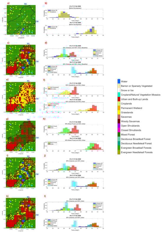
Figure 3.
Spatial distributions of LULC (left column) and category-wise surface air temperature probability distributions (right column) at 01:00 and 16:00 local time for the Nusantara area domain for different scenarios: scenario 1 (a,b), scenario 2 (c,d), scenario 3 (e,f), scenario 4 (g,h), scenario 5 (i,j), and scenario 6 (k,l). The dashed lines indicate the north–south (NS) and east–west (EW) cross-sections used in Figure 4.
Figure 3d shows the baseline scenario that is aligned with the master plan outlined in the IKN law. During nighttime EBF, grasslands and water bodies (WBs) are the colder LULCs in the Nusantara domain, with temperatures ranging from 22 to 26 °C, and urban LULC areas are the hottest, with temperatures ranging from 26 to 27 °C. Notably, the WBs represent a narrower range of temperature differences in the domain, with 60% of the WBs having temperatures between 25 °C and 26 °C. Moreover, during the daytime in the baseline scenario, an increase in the air surface temperature is visible, as shown in Figure 3d. The WB slightly increased in temperature to 26.5–27 °C. Moreover, the EBF areas presented a significant increase in the air temperature of approximately 5.5 °C compared with the nighttime temperature.
Therefore, implementing the Nusantara capital city is projected to accelerate the increase in the urban temperature at night by expanding the warmed urban areas. In scenarios 2–4, despite the built-up areas occupying the same proportion (50%), with the remaining 50% allocated to strategic green spaces, the peak air temperatures within the built-up areas consistently remained at 27 °C (Figure 3d,f,h). A similar pattern was observed in scenarios 5–6, where the built-up areas constituted 35% and 65%, yet the peak air temperatures again remained at 27.5–28 °C (Figure 3j,l). These results suggest that the green strategies proposed in the master plan may not effectively reduce nighttime temperatures across all built-up areas.
At 16:00, the air temperature across all land categories significantly increased compared with the ranges observed at 01:00, except for water bodies. The differences in peak air temperatures between built-up areas and other vegetated areas narrow across all scenarios. The built-up areas exhibit a peak proportion of approximately 40% at 30.5 °C. Although the proportions of air temperatures at the peak remain consistent in scenarios 2–6, the specific amounts vary depending on the scenario. In scenarios 2, 4, 5, and 6, the proportion of areas experiencing peak temperatures in urban regions is smaller than those in water bodies and mixed forests (Figure 3b,d,f,h). This suggests that while urban areas tend to have higher temperatures, they occupy a relatively smaller portion of the landscape than do water bodies and mixed forests.
3.3. Cross-Sectional Winds and Temperature Profile
Figure 4 depicts the differences in surface air temperature (Temp) and wind speed (WS) before and after Nusantara city developed along the east–west (EW) and north–south (NS) cross-sections. Scenario 1 represents the predevelopment LULC condition, whereas scenarios 2 to 6 are the post-development conditions of Nusantara city. In the simulations, mitigation measures were applied to scenarios 2–6 by adjusting albedo values to 0.8 for roofs and 0.7 for walls in urban areas. As noted, scenario 1 did not include any urban land within the focused area, KIPP. Thus, each panel presents the air temperature and wind speed differences at the EW and NS cross-sections between scenario 1 and scenarios 2 to 6, including the differences at night (01:00) and day (16:00) times. In addition, Figure A2 depicts the paired comparisons of surface air temperature and wind speed at the EW and NS cross-sections before and after city development, and Figure A3 presents the spatial wind patterns at nighttime and daytime on 21 October 2020, the hottest day of a year, over the city area. In general, as shown in Figure 4, variations in LULC significantly affect the surface air temperature and wind speed across the region.
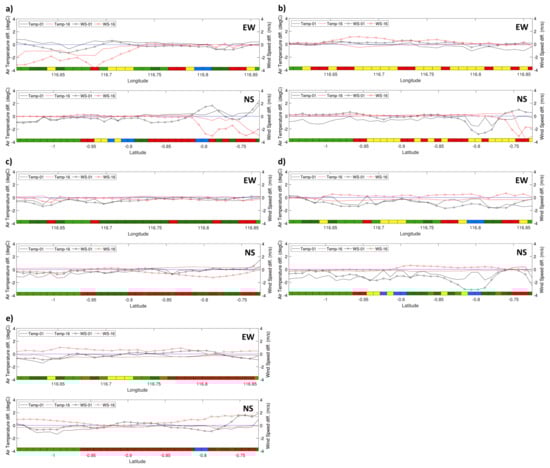
Figure 4.
Differences in surface air temperature (Temp) and wind speed (WS) at 01:00 and 16:00 local time at the east–west (EW) and north–south (NS) cross-sections before (scenario 1) and after (scenarios 2–6) Nusantara city development; Temp and WS differences (a) between scenario 1 and scenario 2, (b) between scenario 1 and scenario 3, (c) between scenario 1 and scenario 4, (d) between scenario 1 and scenario 5, and (e) between scenario 1 and scenario 6. Figure 3 shows the locations of the EW and NS cross-sections. The mitigation measures were incorporated into scenarios 2–6 by adjusting the albedo values to 0.8 for roofs and 0.7 for walls. (For references to color blocks in this figure legend, please see Figure 3).
In particular, land covers dominated by vegetation, such as EBF, mixed forests, and grasslands, typically experience lower temperatures than built-up areas do, with an average temperature reduction of approximately 1 °C (Figure 4b,c). Vegetation exerts a cooling effect through processes such as transpiration, where plants release water vapor into the atmosphere, and through the provision of shade, which mitigates surface heating by solar radiation. However, dense vegetation, such as mixed forests, typically impedes wind flow, reducing wind speeds.
Built-up areas tend to absorb and retain more heat with more anthropogenic heat flux, contributing to the UHI effect. This phenomenon results in elevated air temperatures in urban areas (Figure 4a–e). In urban environments, built-up areas create intricate wind patterns. Wind speeds may accelerate when funneled through narrow passages, such as alleys, or between tall buildings, known as the canyon effect.
Water bodies possess relatively high heat capacities, leading to relatively stable temperature regimes. During the day, the water temperatures are generally lower than those of the surrounding land surfaces (Figure 4a,d,e). However, at night, water bodies release stored heat gradually, warming adjacent areas relative to the land. Large water bodies generally exhibit relatively high and consistent wind speeds because of the absence of significant physical obstructions. The wind direction over water surfaces also tends to be more uniform than the variability observed over heterogeneous land terrains, as depicted in Figure A3.
3.4. Land Surface Temperature Comparison
To assess the effectiveness of green space in reducing urban-induced surface air temperature in IKNs, scenario 2, which is based on IKN regulations with 50% green space and 50% built-up areas, was analyzed as a baseline condition. At the EW1 cross-section at −0.97° S (Figure 5A), the daytime surface temperature peaked at 31.5 °C in the built-up areas (116.6–116.74° E), with a minimum of 26 °C over the water bodies. The wind speed ranged from 3 to 4.2 m/s. At night, air temperatures vary from 24 °C in forest areas to 26 °C in built-up regions, with wind speeds between 1.75 and 4 m/s. Similarly, the EW2 cross-section at −0.82° S (Figure 5B) presented a maximum daytime temperature of 31.5 °C in built-up areas and a minimum of 28 °C. The wind speed ranged from 3 to 5 m/s during the daytime and 0.5 to 5.8 m/s during the nighttime. Along the NS1 cross-section at 116.69° E (Figure 5C), the daytime temperature reached 30.5 °C in built-up areas, with a low temperature of 27 °C in forested regions. The wind speed varied between 2.5 and 4.1 m/s. At night, temperatures range from 22 °C in forests to 27 °C in urban areas, with wind speeds ranging from 0.5 to 5 m/s. The NS2 cross-section at 116.74° E (Figure 5D) has a daytime high of 31 °C and a minimum of 29.8 °C over water bodies, with wind speeds ranging from 3.5 to 5 m/s. Nighttime temperatures ranged from 24 °C in forested areas to 27 °C in urban zones, with wind speeds ranging from 0.75 to 5.8 m/s.
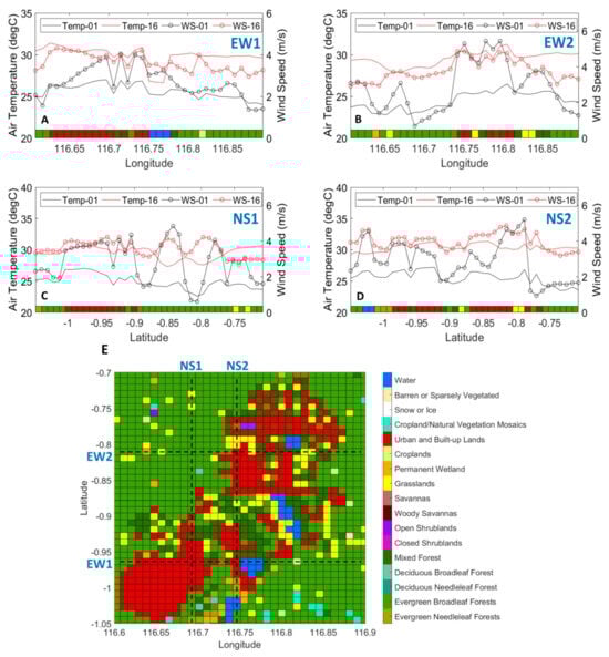
Figure 5.
Comparisons of the simulated surface air temperature (Temp) and wind speed (WS) from scenario 2 at 01:00 and 16:00 local time along (A) EW1, (B) EW2, (C) NS1, and (D) NS2 cross-sections and (E) the LULC pattern of scenario 2 with the locations of the cross-sections.
When surface air temperatures were compared, the built-up areas in mixed forests and EBF presented temperatures up to 1 °C lower than those in EBF. However, when winds traverse a water body before it enters the EBF classification, it results in additional cooling of approximately 2.4 °C (Figure 5A). Notably, the cooling effect of water bodies can further reduce surface air temperatures as the air moves from built-up areas into other land categories (Figure 5A). This observation highlights the significant influence of water bodies in modulating temperature in adjacent land uses. Built-up surfaces typically have a higher albedo, reflecting a greater proportion of incoming sunlight. In contrast, vegetation has a lower albedo and thus absorbs more solar radiation and heat. The upper surfaces of vegetation canopies absorb direct sunlight more effectively than the often reflective or flat surfaces of built-up areas do. This absorption can result in higher temperatures on the canopy surface during the day than in built-up areas, which generally experience a more uniform heat distribution (Figure 5C).
3.5. Effects of the Water Body
Figure 6 shows the average hourly surface air temperature variations over computational domain 3 on the hottest day, 21 October 2020, with and without water bodies and the differences between them. In scenarios 2, 5, and 6 in Figure 6c, the variation in the difference in surface air temperature and wind speed is clearly influenced by the presence of the water body (blue) infrastructure. The difference in surface air temperature between water bodies with and without water bodies during the day and night is consistently negative, indicating cooler conditions. This finding aligns with those of previous studies by Sanusi and Jalil (2021) [52] and Mitchell et al. (2022) [53], which suggest that a larger blue and green infrastructure composition can be more effective in urban cooling. Water bodies and green infrastructure contribute to mitigating UHI effects. Water bodies generally provide a stronger and more consistent cooling effect. However, the choice between blue and green infrastructure often depends on local conditions, available space, and additional desired benefits beyond cooling.
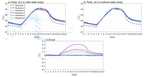
Figure 6.
Comparison of the average hourly surface air temperature over computational domain 3 for various scenarios (a) with water bodies, (b) without water bodies, and (c) the difference in air temperature between (b) and (a).
Compared with vegetation, water bodies are generally considered more effective and resilient in mitigating UHI effects [54]. In terms of the cooling mechanism, water bodies primarily cool through evaporation and heat absorption [52], and green infrastructure cools through evapotranspiration, shading, and thermal insulation [55]. The temporal effectiveness of water bodies can maintain their cooling effect more consistently, including at night (Figure 6a). However, some green infrastructure, such as grasslands, may have a warming effect during the day [52].
The seasonal impact of water bodies is most effective in summer when solar radiation is strong. Moreover, the effectiveness of green infrastructure can vary seasonally, with deciduous vegetation being less effective in winter. Water bodies and green infrastructure offer ecosystem services beyond cooling, such as stormwater management and biodiversity support [11,24]. Moreover, implementation challenges also occur. Water bodies may require more space and have higher implementation costs, and green infrastructure can be more easily integrated into existing urban structures (e.g., green roofs and street trees).
4. Conclusions
This study assessed the impact of green and mitigation strategies for urban cooling on the development of Nusantara Capital City, Indonesia. These findings indicate that the development of Nusantara will result in a substantial rise in surface air temperatures. However, the implementation of effective mitigation measures (for example, roof material with high albedo) has the potential to significantly reduce the increase in air temperature. On the basis of simulations that explored different LULC scenarios, the key conclusions of this study are as follows:
- The cooling effects in built-up areas vary significantly across different scenarios. Scenarios 2, 5, and 6, which incorporate LULC with blue–green infrastructure, exhibit the most substantial reductions in surface air temperature because of their ability to mitigate UHI effects. Conversely, scenarios 3 and 4, which feature grasslands and mixed forest LULC, show the least cooling effects and, in some cases, even higher air temperatures and wind speeds than scenarios without blue–green infrastructure. As noted earlier, mitigation measures were also incorporated into scenarios 2–6 by modifying the albedo values of urban areas to 0.8 for roofs and 0.7 for walls.
- The study further highlights that, in the case of Nusantara, mixed forests are generally more effective than grasslands in mitigating adverse urban microclimatic impacts. Mixed forests provide better cooling effects because of their greater evapotranspiration capacity, which is driven by greater leaf area and vegetation density. The tree canopy in mixed forests offers significant shading, which reduces surface temperatures, whereas grasslands, with minimal shading, contribute less to cooling. Additionally, grasslands, which are characterized by low-lying vegetation, absorb and release heat differently, limiting their ability to buffer temperature fluctuations compared with the vertical structure of forests.
- Among all the LULC scenarios, scenario 5, which included the highest proportion of blue–green spaces (65%), exhibited the most significant urban cooling effect. This scenario has the potential to reduce the average surface air temperature by approximately 2 °C, outperforming the other scenarios.
- The simulation results for scenario 2 show that wind passing over a water body before entering EBF areas provides an additional cooling effect of approximately 2.4 °C. This cooling effect further propagates as the air moves from built-up areas into other land types. These findings underscore the critical role of strategically integrating water bodies and blue–green spaces into urban planning to enhance natural cooling and alleviate urban heat, especially in densely developed areas.
The outcomes of this research emphasize that, during the future development of new capital regions, built-up areas need to consider the climatological patterns of wind direction (the wind blows, passing over the lake or urban forest before reaching the built-up areas). This is important because establishing blue–green infrastructure around built-up areas can create a more efficient passive cooling environment. Scenario 4 (the combination of mixed forest and built-up areas) resulted in the smallest difference in the air temperature variations. This is probably because the composition consists of tall trees and woody vegetation with leafy types surrounding the built-up areas. Moreover, a large difference in air temperature variation in terms of the most efficient cooling rates is achieved by scenario 5, which consists of 65% blue–green infrastructure.
The findings of this study underscore the critical role of incorporating blue–green infrastructure, such as water bodies and mixed forests, in urban planning to mitigate rising surface air temperatures. For policymakers, this highlights the need to prioritize nature-based solutions in city development, particularly for Nusantara city in Indonesia, to increase urban cooling, reduce UHI effects, and ensure sustainable and climate-resilient growth.
Author Contributions
R.P.P.: writing—original draft, visualization, validation, software, resources, methodology, investigation, formal analysis, data curation, and conceptualization; H.S.L., T.K. and H.N.: writing—original draft, writing—review and editing, validation, supervision, resources, project administration, methodology, investigation, formal analysis, data curation, and conceptualization; V.B., F.R.F., M.R.B. and W.H.: formal analysis, software, visualization, and data curation; I.D.G.A.P.: formal analysis and data curation. All authors have read and agreed to the published version of the manuscript.
Funding
This research was supported by the Science and Technology Research Partnership for Sustainable Development (SATREPS) in collaboration with the Japan Science and Technology Agency (JST, JPMJSA1904) and the Japan International Cooperation Agency (JICA).
Data Availability Statement
All the data used in this study, including hourly records of air temperature at the Sepinggan Balikpapan Meteorological Station, are available from the authors upon request.
Acknowledgments
This research was conducted by the Climate Research Group for the Development of Standard Weather Data as part of the Development of Low-Carbon Affordable Apartments in the Hot-Humid Climate of Indonesia Project toward the Paris Agreement 2030, Science and Technology Research Partnership for Sustainable Development (SATREPS), which is collaboratively supported by the Japan Science and Technology Agency (JST), the Japan International Cooperation Agency (JICA), Hiroshima University, Kagoshima University, the Ministry of Public Works and Housing (PUPR) of Indonesia, and the Indonesian Agency for Meteorology Climatology and Geophysics (BMKG).
Conflicts of Interest
The authors declare that they have no conflicts of interest.
Appendix A
The dry season in the study area was identified as the hottest period, with October being the peak month when surface air temperature reached 28.5°C between 2016 and 2020 (indicated by the red circle (Figure A1b)). In contrast, the wet season recorded the highest rainfall in January and March, reaching 247 mm over the same five-year period (Figure A1 [Appendix A]). For this study, the model was run for 21 days, from 10 October to 31 October 2020. This period was chosen to assess the maximum impact, as October 2020 recorded the highest surface air temperature of the year (Figure A1a,b).

Figure A1.
(a) Observed monthly variations in rainfall and surface air temperature in the study area from Jan 2016–Dec 2020, and (b) the highest average surface air temperature occurred on 21 October 2020 during the five-year period, as indicated by the red circle.
Figure A1.
(a) Observed monthly variations in rainfall and surface air temperature in the study area from Jan 2016–Dec 2020, and (b) the highest average surface air temperature occurred on 21 October 2020 during the five-year period, as indicated by the red circle.

Figure A2 depicts the paired comparison of surface air temperature (Temp) and wind speed (WS) at 01:00 and 16:00 local time along the east–west (EW) and north–south (NS) cross-sections for each scenario.
The difference in air temperature for scenario 2 is 1.5 °C in the built-up areas during the day and 1 °C at night over the expanded built-up areas across the NS cross-section (Figure A2a,b). Moreover, in scenario 3, the temperature slightly decreased to 0.1 °C (EW) and 2.1 °C (NS) (Figure A2c,d). Then, scenario 4 shows a small deviation in the air temperature, which is approximately 0.1 °C (for EW and NS) during the day and night (Figure A2e,f).
However, scenario 5 (Figure A2g,h) has the opposite value of air temperature difference, which reduces the air temperature by up to 0.2 °C in the daytime (EW) but increases it by up to 0.2 °C over the expanded built-up areas (NS).
In scenario 6, as the highest built-up area, which accounts for 65% of the total area, the air temperature difference during the daytime can be reduced by up to 0.2 °C (EW). Moreover, in the NS cross-section, it decreased by up to 0.1 °C (Figure A2i,j).


Figure A2.
Paired comparison of simulated surface air temperature with wind speed before and after Nusantara city development: scenario 2 (a,b), scenario 3 (c,d), scenario 4 (e,f), scenario 5 (g,h), and scenario 6 (i,j). (For references to color blocks in this figure legend, please see Figure 3).
Figure A2.
Paired comparison of simulated surface air temperature with wind speed before and after Nusantara city development: scenario 2 (a,b), scenario 3 (c,d), scenario 4 (e,f), scenario 5 (g,h), and scenario 6 (i,j). (For references to color blocks in this figure legend, please see Figure 3).


Figure A3 shows spatial wind patterns at 01:00 (nighttime) and 16:00 (daytime) to highlight the variations in wind speed and direction across different land use and land cover types on 21 October 2020.

Figure A3.
Spatial wind patterns at 01:00 and 16:00 local time on 21 October 2020. (For references to color blocks in this figure legend, please see Figure 3).
Figure A3.
Spatial wind patterns at 01:00 and 16:00 local time on 21 October 2020. (For references to color blocks in this figure legend, please see Figure 3).

References
- Elmqvist, T.; Fragkias, M.; Goodness, J.; Güneralp, B.; Marcotullio, P.J.; McDonald, R.I.; Parnell, S.; Schewenius, M.; Sendstad, M.; Seto, K.C.; et al. Urbanization, Biodiversity and Ecosystem Services: Challenges and Opportunities: A Global Assessment; Springer: Dordrecht, The Netherlands, 2013; pp. 1–755. [Google Scholar] [CrossRef]
- Bhanage, V.; Kulkarni, S.; Sharma, R.; Lee, H.S.; Gedam, S. Enumerating and Modelling the Seasonal alterations of Surface Urban Heat and Cool Island: A Case Study over Indian Cities. Urban Sci. 2023, 7, 38. [Google Scholar] [CrossRef]
- Bhati, S.; Mohan, M. WRF model evaluation for the urban heat island assessment under varying land use/land cover and reference site conditions. Theor. Appl. Clim. 2016, 126, 385–400. [Google Scholar] [CrossRef]
- Doan, Q.; Kusaka, H. Numerical study on regional climate change due to the rapid urbanization of greater Ho Chi Minh City’s metropolitan area over the past 20 years. Int. J. Clim. 2016, 36, 3633–3650. [Google Scholar] [CrossRef]
- Dwivedi, A. Macro- and micro-level studies using Urban Heat Islands to simulate effects of greening, building materials and other mitigating factors in Mumbai city. Arch. Sci. Rev. 2019, 62, 126–144. [Google Scholar] [CrossRef]
- Dwivedi, A.; Khire, M. Application of split- window algorithm to study Urban Heat Island effect in Mumbai through land surface temperature approach. Sustain. Cities Soc. 2018, 41, 865–877. [Google Scholar] [CrossRef]
- Dwivedi, A.; Mohan, B.K. Impact of green roof on micro climate to reduce Urban Heat Island. Remote. Sens. Appl. Soc. Environ. 2018, 10, 56–69. [Google Scholar] [CrossRef]
- Al Kafy, A.; Faisal, A.A.; Rahman, S.; Islam, M.; Al Rakib, A.; Islam, A.; Khan, H.H.; Sikdar, S.; Sarker, H.S.; Mawa, J.; et al. Prediction of seasonal urban thermal field variance index using machine learning algorithms in Cumilla, Bangladesh. Sustain. Cities Soc. 2021, 64, 102542. [Google Scholar] [CrossRef]
- Kant, Y.; Bharath, B.D.; Mallick, J.; Atzberger, C.; Kerle, N. Satellite-based analysis of the role of land use/land cover and vegetation density on surface temperature regime of Delhi, India. J. Indian Soc. Remote Sens. 2009, 37, 201–214. [Google Scholar] [CrossRef]
- Demisse Negesse, M.; Hishe, S.; Getahun, K. LULC dynamics and the effects of urban green spaces in cooling and mitigating micro-climate change and urban heat island effects: A case study in Addis Ababa City, Ethiopia. J. Water Clim. Change 2024, 15, 3033–3055. [Google Scholar] [CrossRef]
- Uddin, A.S.M.S.; Khan, N.; Islam, A.R.M.T.; Kamruzzaman, M.; Shahid, S. Changes in urbanization and urban heat island effect in Dhaka city. Theor. Appl. Clim. 2022, 147, 891–907. [Google Scholar] [CrossRef]
- Mensah, C.; Atayi, J.; Kabo-Bah, A.T.; Švik, M.; Acheampong, D.; Kyere-Boateng, R.; Prempeh, N.A.; Marek, M.V. Impact of urban land cover change on the garden city status and land surface temperature of Kumasi. Cogent Environ. Sci. 2020, 6, 1787738. [Google Scholar] [CrossRef]
- Hassan, T.; Zhang, J.; Prodhan, F.A.; Sharma, T.P.P.; Bashir, B. Surface Urban Heat Islands Dynamics in Response to LULC and Vegetation across South Asia (2000–2019). Remote. Sens. 2021, 13, 3177. [Google Scholar] [CrossRef]
- Shi, Z.; Li, X.; Hu, T.; Yuan, B.; Yin, P.; Jiang, D. Modeling the intensity of surface urban heat island based on the impervious surface area. Urban Clim. 2023, 49, 101529. [Google Scholar] [CrossRef]
- Weng, Q.; Rajasekar, U.; Hu, X. Modeling urban heat islands and their relationship with impervious surface and vegetation abundance by using ASTER images. IEEE Trans. Geosci. Remote Sens. 2011, 49, 4080–4089. [Google Scholar] [CrossRef]
- Yuan, F.; Bauer, M.E. Comparison of impervious surface area and normalized difference vegetation index as indicators of surface urban heat island effects in Landsat imagery. Remote Sens. Environ. 2007, 106, 375–386. [Google Scholar] [CrossRef]
- Ahmed, H.A.; Singh, S.K.; Kumar, M.; Maina, M.S.; Dzwairo, R.; Lal, D. Impact of urbanization and land cover change on urban climate: Case study of Nigeria. Urban Clim. 2020, 32, 100600. [Google Scholar] [CrossRef]
- Heaviside, C.; Vardoulakis, S.; Cai, X.-M. Attribution of mortality to the urban heat island during heatwaves in the West Midlands, UK. Environ. Health A Glob. Access Sci. Source 2016, 15 (Suppl. S1), 49–59. [Google Scholar] [CrossRef]
- Yang, J.; Santamouris, M. Urban Heat Island and Mitigation Technologies in Asian and Australian Cities—Impact and Mitigation. Urban Sci. 2018, 2, 74. [Google Scholar] [CrossRef]
- Feizizadeh, B.; Blaschke, T. Examining Urban Heat Island Relations to Land Use and Air Pollution: Multiple Endmember Spectral Mixture Analysis for Thermal Remote Sensing. IEEE J. Sel. Top. Appl. Earth Obs. Remote. Sens. 2013, 6, 1749–1756. [Google Scholar] [CrossRef]
- Sarrat, C.; Lemonsu, A.; Masson, V.; Guédalia, D. Impact of urban heat island on regional atmospheric pollution. Atmos. Environ. 2006, 40, 1743–1758. [Google Scholar] [CrossRef]
- Li, H.; Harvey, J.T.; Holland, T.J.; Kayhanian, M. Corrigendum: The use of reflective and permeable pavements as a potential practice for heat island mitigation and stormwater management. Environ. Res. Lett. 2013, 8, 049501. [Google Scholar] [CrossRef]
- Gasparrini, A.; Guo, Y.; Hashizume, M.; Lavigne, E.; Zanobetti, A.; Schwartz, J.; Tobias, A.; Tong, S.; Rocklöv, J.; Forsberg, B.; et al. Mortality risk attributable to high and low ambient temperature: A multicountry observational study. Lancet 2015, 386, 369–375. [Google Scholar] [CrossRef] [PubMed]
- Lestari, S.; Syamsudin, F.; Pianto, T.A.; Sulistyowati, R.; Yulihastin, E.; Nugroho, D.; Hatmaja, R.B.; Amrina, D.; Habibi, M.N. Comparison of Statistical Properties of Rainfall Extremes Between Megacity Jakarta and New Capital City Nusantara. Springer Proc. Phys. 2023, 290, 325–334. [Google Scholar] [CrossRef]
- Ramadhan, R.; Marzuki, M.; Suryanto, W.; Sholihun, S.; Yusnaini, H.; Muharsyah, R.; Hanif, M. Trends in rainfall and hydrometeorological disasters in new capital city of Indonesia from long-term satellite-based precipitation products. Remote. Sens. Appl. Soc. Environ. 2022, 28, 100827. [Google Scholar] [CrossRef]
- Purwaningsih, A.; Lubis, S.W.; Hermawan, E.; Andarini, D.F.; Harjana, T.; Ratri, D.N.; Ridho, A.; Risyanto; Sujalu, A.P. Moisture Origin and Transport for Extreme Precipitation over Indonesia’s New Capital City, Nusantara in August 2021. Atmosphere 2022, 13, 1391. [Google Scholar] [CrossRef]
- Sofan, P.; Rahmi, K.I.N.; Sari, N.M.; Nugroho, J.T.; Wati, T.; Sakti, A.D. Modeling the Surface Thermal Discomfort Index (STDI) in a Tropical Environments using Multi Sensors: A Case Study of East Kalimantan, The Future New Capital City of Indonesia. J. Indian Soc. Remote. Sens. 2024, 52, 1761–1776. [Google Scholar] [CrossRef]
- Tursilowati, L.; Sunarya, R.; Muzirwan; Maryadi, E.; Susanti, I.; Rahayu, S.A. Seasonal Urban Heat Island Observation Using Remote Sensing and Google Earth Engine in the New Capital of Indonesia. J. Southwest Jiaotong Univ. 2023, 58, 1200–1218. [Google Scholar] [CrossRef]
- Denryanto, R.A.F.; Virgianto, R.H. The impact of land cover changes on temperature parameters in new capital of Indonesia (IKN). IOP Conf. Ser. Earth Environ. Sci. 2021, 893, 012033. [Google Scholar] [CrossRef]
- Sen, S.; Roesler, J.; Ruddell, B.; Middel, A. Cool Pavement Strategies for Urban Heat Island Mitigation in Suburban Phoenix, Arizona. Sustainability 2019, 11, 4452. [Google Scholar] [CrossRef]
- Marando, F.; Heris, M.P.; Zulian, G.; Udías, A.; Mentaschi, L.; Chrysoulakis, N.; Parastatidis, D.; Maes, J. Urban heat island mitigation by green infrastructure in European Functional Urban Areas. Sustain. Cities Soc. 2022, 77, 103564. [Google Scholar] [CrossRef]
- Kubota, T.; Lee, H.S.; Trihamdani, A.R.; Phuong, T.T.T.; Tanaka, T.; Matsuo, K. Impacts of land use changes from the Hanoi Master Plan 2030 on urban heat islands: Part 1. Cooling effects of proposed green strategies. Sustain. Cities Soc. 2017, 32, 295–317. [Google Scholar] [CrossRef]
- Vinayak, B.; Lee, H.S.; Gedam, S.; Latha, R. Impacts of future urbanization on urban microclimate and thermal comfort over the Mumbai metropolitan region, India. Sustain. Cities Soc. 2022, 79, 103703. [Google Scholar] [CrossRef]
- Pradana, R.P. Impacts of the Asian Australian Monsoon and Indo Pacific Sea Surface Temperature on Urban Climates in Major Indonesian Cities for Low Carbon Building Design. Adv. Hydrol. Meteorol. 2024, 1, 1–5. [Google Scholar] [CrossRef]
- Sulla-menashe, D.; Friedl, M.A. User Guide to Collection 6 MODIS Land Cover (MCD12Q1 and MCD12C1) Product. No. Figure 1; Usgs: Reston, VA, USA, 2018; pp. 1–18. [Google Scholar]
- Berawi, M.A. City of Tomorrow: The New Capital City of Indonesia. Int. J. Technol. 2022, 13, 690–694. [Google Scholar] [CrossRef]
- Hong, S.; Lim, J. The WRF single-moment 6-class microphysics scheme (WSM6). J. Korean Meteorol. Soc. 2006, 42, 129–151. [Google Scholar]
- Nakanishi, M.; Niino, H. An Improved Mellor-Yamada Level-3 Model: Its Numerical Stability and Application to a Regional Prediction of Advection Fog. Bound.-Layer Meteorol. 2006, 119, 397–407. [Google Scholar] [CrossRef]
- Zhang, C.; Wang, Y. Projected Future Changes of Tropical Cyclone Activity over the Western North and South Pacific in a 20-km-Mesh Regional Climate Model. J. Clim. 2017, 30, 5923–5941. [Google Scholar] [CrossRef]
- Iacono, M.J.; Delamere, J.S.; Mlawer, E.J.; Shephard, M.W.; Clough, S.A.; Collins, W.D. Radiative forcing by long-lived greenhouse gases: Calculations with the AER radiative transfer models. J. Geophys. Res. Atmos. 2008, 113, 2–9. [Google Scholar] [CrossRef]
- Tewari, M.; Chen, F.; Kusaka, H.; Miao, S. Coupled WRF/Unified Noah/Urban-Canopy Modeling System. NCAR WRF Doc. 2007; pp. 1–20. Available online: http://www.ral.ucar.edu/research/land/technology/urban/WRF-LSM-Urban.pdf (accessed on 20 September 2024).
- Paulson, C.A. The mathematical representation of wind speed and temperature profiles in the unstable atmospheric surface layer. J. Appl. Meteorol. 1970, 9, 857–861. [Google Scholar] [CrossRef]
- Chen, F.; Kusaka, H.; Bornstein, R.; Ching, J.; Grimmond, S.; Grossman-Clarke, S.; Loridan, T.; Manning, K.W.; Martilli, A.; Miao, S.; et al. The integrated WRF/urban modelling system: Development, evaluation, and applications to urban environmental problems. Int. J. Clim. 2011, 31, 273–288. [Google Scholar] [CrossRef]
- Chisale, S.W.; Lee, H.S.; Calvo, M.A.S.; Jeong, J.-S.; Aljber, M.; Williams, Z.; Cabrera, J.S. Advanced solar energy potential assessment in Malawi: Utilizing high-resolution WRF model and GIS to identify optimal sites for solar PV generation. Renew. Energy 2025, 239, 122084. [Google Scholar] [CrossRef]
- Ott, R.L.; Longnecker, M. An Introduction to Statistical Methods and Data Analysis, 6th ed.; Texas A&M University: College Station, TX, USA; Brooks/Cole: Pacific Grove, CA, USA, 2010; ISBN 13: 978-0-495-01758-5. [Google Scholar]
- Pallant, J. SPSS Survival Manual; Taylor & Francis: London, UK, 2020. [Google Scholar] [CrossRef]
- Tursilowati, L.; Sumantyo, J.T.S.; Kuze, H.; Adiningsih, E.S. The integrated WRF/Urban modeling system and its application to monitoring urban heat island in Jakarta-Indonesia. J. Urban Environ. Eng. 2012, 6, 1–9. [Google Scholar] [CrossRef][Green Version]
- Jankov, I.; Gallus, W.A.; Segal, M.; Shaw, B.; Koch, S.E. The Impact of Different WRF Model Physical Parameterizations and Their Interactions on Warm Season MCS Rainfall. Weather Forecast. 2005, 20, 1048–1060. [Google Scholar] [CrossRef]
- Crétat, J.; Pohl, B.; Richard, Y.; Drobinski, P. Uncertainties in simulating regional climate of Southern Africa: Sensitivity to physical parameterizations using WRF. Clim. Dyn. 2012, 38, 613–634. [Google Scholar] [CrossRef]
- Yang, B.; Qian, Y.; Lin, G.; Leung, R.; Zhang, Y. Some issues in uncertainty quantification and parameter tuning: A case study of convective parameterization scheme in the WRF regional climate model. Atmos. Meas. Tech. 2012, 12, 2409–2427. [Google Scholar] [CrossRef]
- Wang, Z.-H.; Bou-Zeid, E.; Au, S.K.; Smith, J.A. Analyzing the Sensitivity of WRF’s Single-Layer Urban Canopy Model to Parameter Uncertainty Using Advanced Monte Carlo Simulation. J. Appl. Meteorol. Clim. 2011, 50, 1795–1814. [Google Scholar] [CrossRef]
- Sanusi, R.; Jalil, M. Blue-Green infrastructure determines the microclimate mitigation potential targeted for urban cooling. IOP Conf. Ser. Earth Environ. Sci. 2020, 918, 012010. [Google Scholar] [CrossRef]
- Mitchell, G.; Chan, F.K.S.; Chen, W.Y.; Thadani, D.R.; Robinson, G.M.; Wang, Z.; Li, L.; Li, X.; Mullins, M.-T.; Chau, P.Y.K. Can green city branding support China’s Sponge City Programme? Blue-Green Syst. 2022, 4, 24–44. [Google Scholar] [CrossRef]
- Balany, F.; Ng, A.W.; Muttil, N.; Muthukumaran, S.; Wong, M.S. Green Infrastructure as an Urban Heat Island Mitigation Strategy—A Review. Water 2020, 12, 3577. [Google Scholar] [CrossRef]
- Kumar, P.; Debele, S.E.; Khalili, S.; Halios, C.H.; Sahani, J.; Aghamohammadi, N.; Andrade, M.d.F.; Athanassiadou, M.; Bhui, K.; Calvillo, N.; et al. Urban heat mitigation by green and blue infrastructure: Drivers, effectiveness, and future needs. Innovation 2024, 5, 100588. [Google Scholar] [CrossRef]


Disclaimer/Publisher’s Note: The statements, opinions and data contained in all publications are solely those of the individual author(s) and contributor(s) and not of MDPI and/or the editor(s). MDPI and/or the editor(s) disclaim responsibility for any injury to people or property resulting from any ideas, methods, instructions or products referred to in the content. |
© 2025 by the authors. Licensee MDPI, Basel, Switzerland. This article is an open access article distributed under the terms and conditions of the Creative Commons Attribution (CC BY) license (https://creativecommons.org/licenses/by/4.0/).