
The Machine Learning Attribution of Quasi-Decadal Precipitation and Temperature Extremes in Southeastern Australia during the 1971–2022 Period


Abstract
1. Introduction
2. Materials and Methods
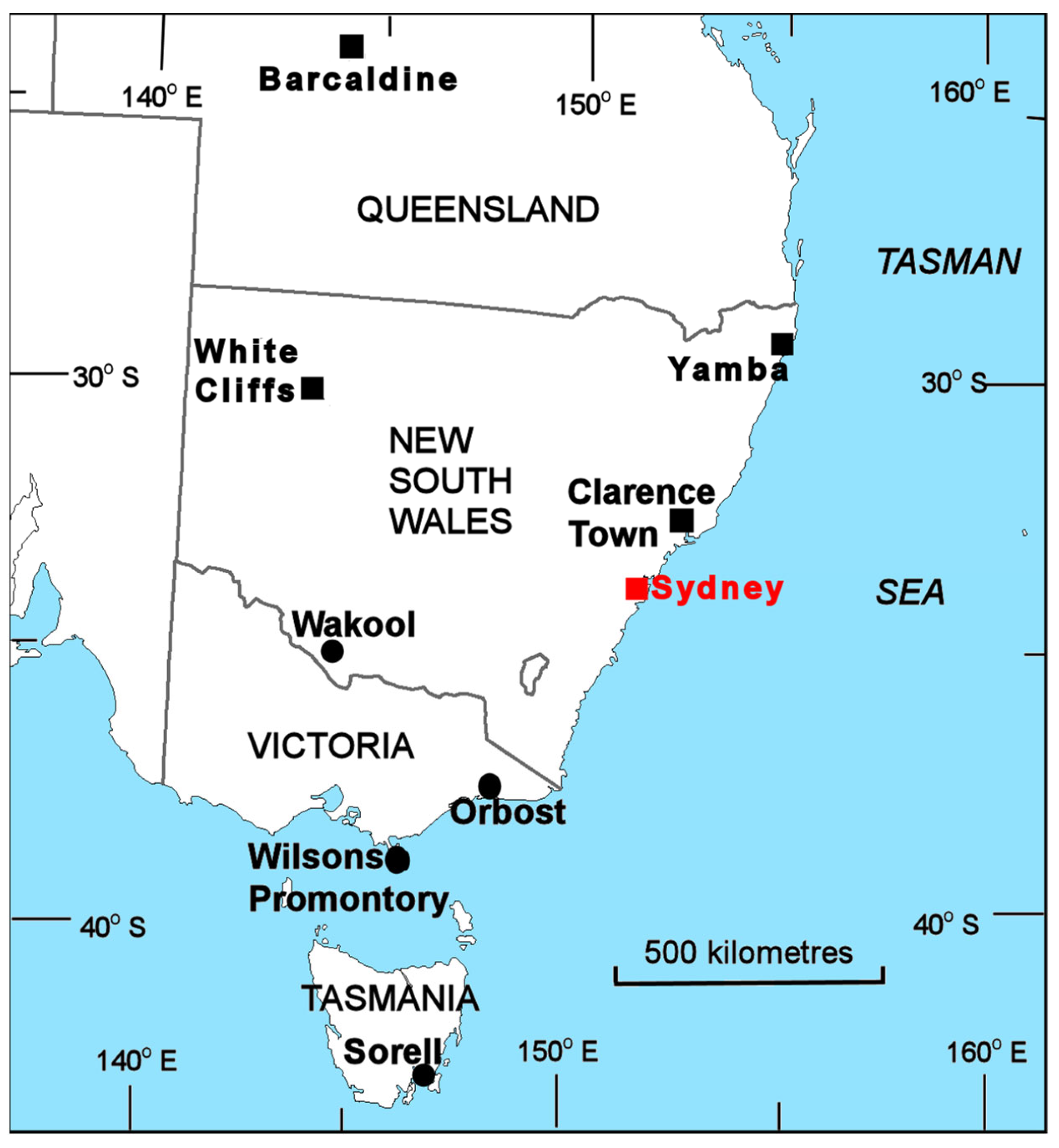
2.1. Study Area
2.2. Data
2.3. Methods
3. Results
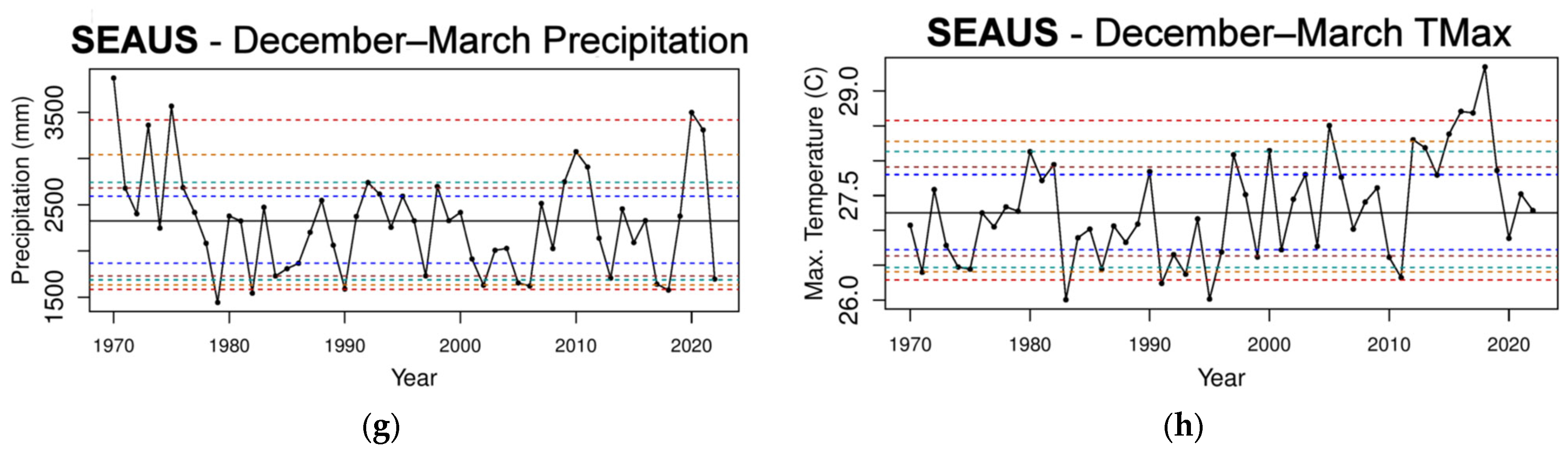
3.1. Precipitation and TMax Time Series for SEAUS
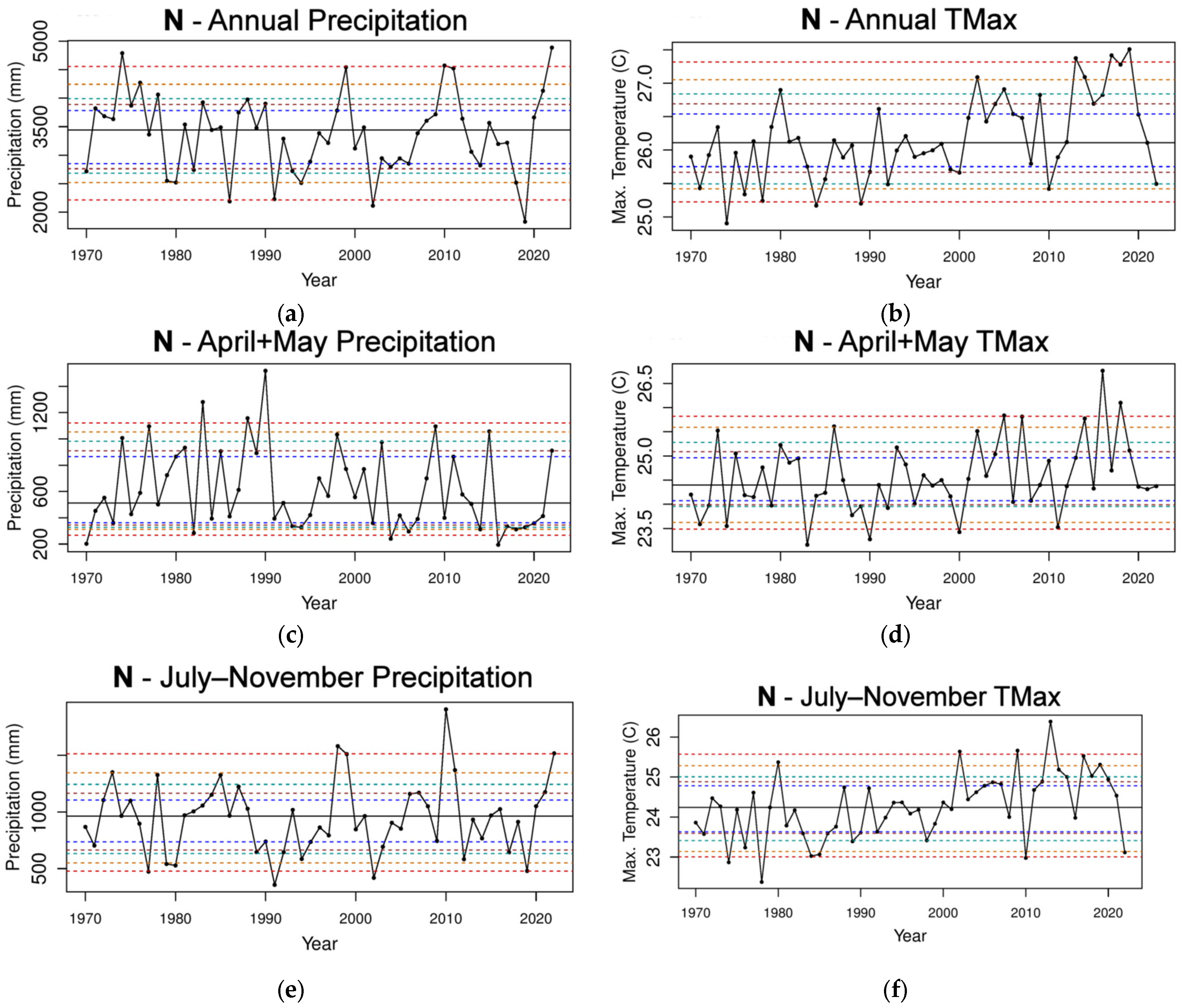
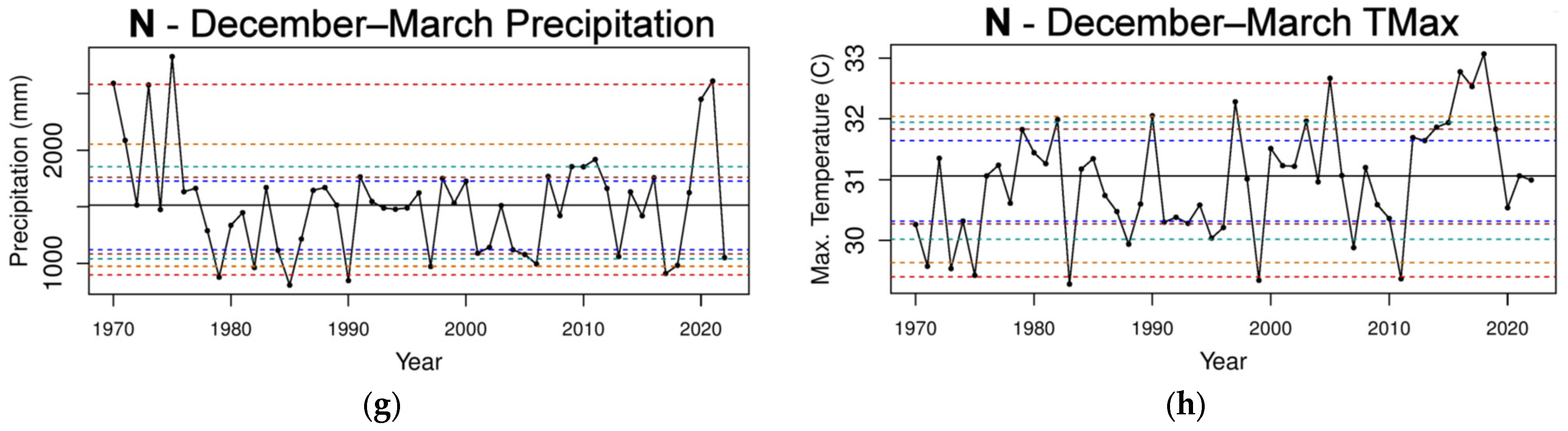
3.2. Total Precipitation and TMax Time Series of N
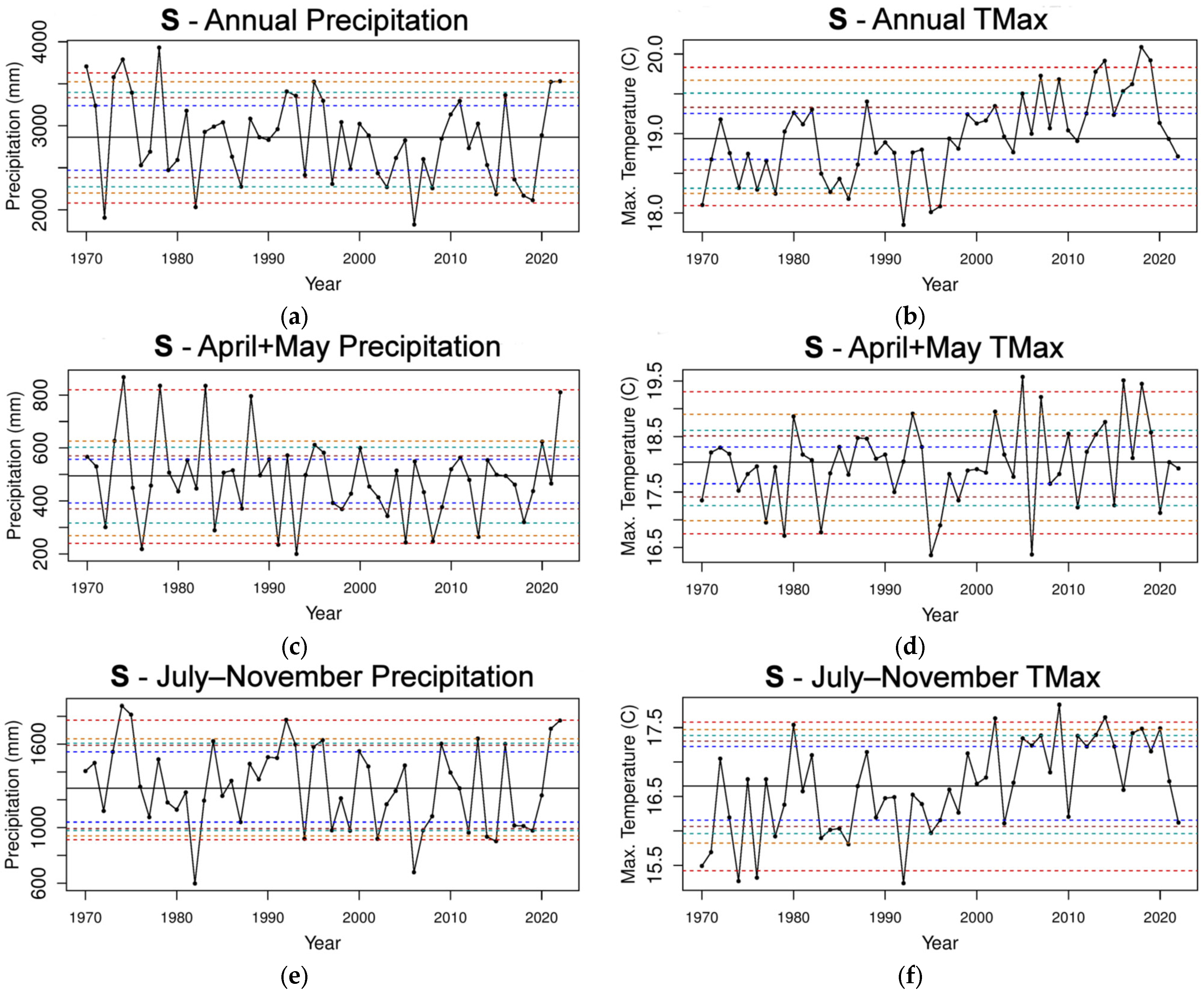
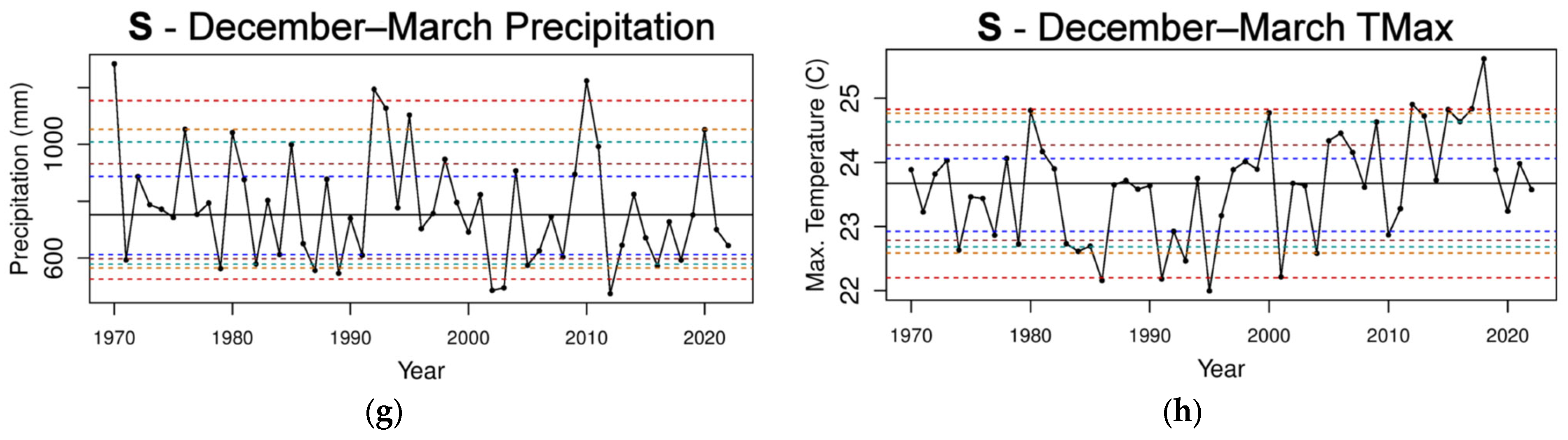
3.3. Total Precipitation and TMax Time Series of S
3.4. Total Precipitation and TMax p-Values for Six Quasi-Decadal Intervals
3.5. Attribute Selection
4. Discussion
5. Conclusions
Supplementary Materials
Author Contributions
Funding
Data Availability Statement
Acknowledgments
Conflicts of Interest
References
- BoM 2020. Australian Bureau of Meteorology and CSIRO. State of the Climate 2020. Available online: https://bom.gov.au/state-of-the-climate/ (accessed on 7 March 2024).
- IPCC. Climate Change 2021: The Physical Science Basis. Contribution of Working Group I to the Sixth Assessment Report of the Intergovernmental Panel on Climate Change; Masson-Delmotte, V., Zhai, P., Pirani, A., Connors, S.L., Péan, C., Chen, Y., Goldfarb, L., Gomis, M.I., Matthews, J.B.R., Berger, S., et al., Eds.; Cambridge University Press: Cambridge, UK; New York, NY, USA, 2021; Available online: https://www.ipcc.ch/report/ar6/wg1/downloads/report/IPCC_AR6_WGI_SPM_final.pdf (accessed on 1 April 2024).
- NOAA. National Centers for Environmental Information, State of the Climate: Global Climate Report for 2019. Available online: https://www.ncdc.noaa.gov/sotc/global/201913/supplemental/page-3 (accessed on 7 March 2024).
- Speer, M.S.; Leslie, L.M.; Fierro, A.O. Australian east coast rainfall decline related to large scale climate drivers. Clim. Dyn. 2011, 36, 1419–1429. [Google Scholar] [CrossRef]
- Speer, M.; Hartigan, J.; Leslie, L. Machine Learning Assessment of the Impact of Global Warming on the Climate Drivers of Water Supply to Australia’s Northern Murray-Darling Basin. Water 2022, 14, 3073. [Google Scholar] [CrossRef]
- National Oceanic and Atmospheric Administration. Thirty-Year Climate Normal. Understanding Climate Normals. Available online: https://www.noaa.gov/explainers/understanding-climate-normals (accessed on 7 May 2024).
- Cheng, L.; AghaKouchak, A. Nonstationary Precipitation Intensity-Duration-Frequency Curves for Infrastructure Design in a Changing Climate. Sci. Rep. 2014, 4, 7093. [Google Scholar] [CrossRef] [PubMed]
- Slater, L.J.; Anderson, B.; Buechel, M.; Dadson, S.; Han, S.; Harrigan, S.; Kelder, T.; Kowal, K.; Lees, T.; Matthews, T.; et al. Nonstationary weather and water extremes: A review of methods for their detection, attribution, and management. Hydrol. Earth Syst. Sci. 2021, 25, 3897–3935. [Google Scholar] [CrossRef]
- Speer, M.; Leslie, L. Southeast Australia encapsulates the recent decade of extreme global weather and climate events. Acad. Environ. Sci. Sustain. 2023, 1. [Google Scholar] [CrossRef]
- Speer, M.; Leslie, L. Application of Machine Learning Techniques to Detect and Understand the Impacts of Global Warming on Southeast Australia. Georget. J. Int. Aff. 2023, 24, 260–266. [Google Scholar] [CrossRef]
- Record-Breaking La Niña Events. Available online: http://www.bom.gov.au/climate/enso/history/La-Nina-2010-12.pdf (accessed on 7 March 2024).
- Understanding the IOD. Available online: http://www.bom.gov.au/climate/about/?bookmark=iod (accessed on 7 March 2024).
- Southern Annular Mode. Available online: http://www.bom.gov.au/climate/about/?bookmark=sam (accessed on 7 March 2024).
- BoM Climate Data. Australian Bureau of Meteorology. Available online: http://www.bom.gov.au/climate/data/ (accessed on 7 March 2024).
- Tasman Sea Surface Temperature Anomalies. Available online: http://www.bom.gov.au/climate/change/?ref=ftr#tabs=Tracker&tracker=timeseries (accessed on 24 April 2024).
- Speer, M.S.; Leslie, L.M.; MacNamara, S.; Hartigan, J. From the 1990s climate change has decreased cool season catchment precipitation reducing river heights in Australia’s southern Murray-Darling Basin. Sci. Rep. 2021, 11, 16136. [Google Scholar] [CrossRef] [PubMed]
- Understanding ENSO. Available online: http://www.bom.gov.au/climate/about/?bookmark=enso (accessed on 7 March 2024).
- Speer, M.; Hartigan, J.; Leslie, L. Machine Learning Identification of Attributes and Predictors for a Flash Drought in Eastern Australia. Climate 2024, 12, 49. [Google Scholar] [CrossRef]
- Brownlee, J. Long Short-Term Memory Networks with Python Develop Sequence Prediction Models with Deep Learning; Machine Learning Mastery EBook: San Juan, PR, USA, 2017. [Google Scholar]
- Maldonado, S.; Weber, R. A wrapper method for feature selection using Support Vector Machines. Inf. Sci. 2009, 179, 2208–2217. [Google Scholar] [CrossRef]
- Annual Deciles of Actual Evapotranspiration 2018–2019. Available online: http://www.bom.gov.au/water/nwa/2019/mdb/climateandwater/climateandwater.shtml (accessed on 7 March 2024).
- Hartigan, J.; MacNamara, S.; Leslie, L.M. Application of machine learning to attribution and prediction of seasonal precipitation and temperature trends in Canberra, Australia. Climate 2020, 8, 76. [Google Scholar] [CrossRef]
- Hartigan, J.; MacNamara, S.; Leslie, L.; Speer, M. Attribution and prediction of precipitation and temperature trends within the Sydney catchment using machine learning. Climate 2020, 8, 120. [Google Scholar] [CrossRef]
- Robinson, A.; Lehmann, J.; Barriopedro, D.; Rahmstorf, S.; Coumou, D. Increasing heat and rainfall extremes now far outside the historical climate. npj Clim. Atmos. Sci. 2021, 4, 45. [Google Scholar] [CrossRef]
- Francis, J.A.; Vavrus, S.J. Evidence linking Arctic amplification to extreme weather in mid-latitudes. Geophys. Res. Lett. 2012, 39, L06801. [Google Scholar] [CrossRef]
- Hendon, H.H.; Thompson, D.W.J.; Wheeler, M.C. Australian Rainfall and Surface Temperature Variations Associated with the Southern Hemisphere Annular Mode. J. Clim. 2007, 20, 2452–2467. [Google Scholar] [CrossRef]
- Lim, E.-P.; Hendon, H.H. Understanding and predicting the strong Southern Annular Mode and its impact on the record wet east Australian spring 2010. Clim Dyn. 2015, 44, 2807–2824. [Google Scholar] [CrossRef]
- Speer, M.; Geerts, B. A synoptic-mesoalpha scale climatology of flash floods in the Sydney metropolitan area. Aust. Meteorol. Mag. 1994, 43, 87–103. [Google Scholar]
- Holland, G.J.; Lynch, A.H.; Leslie, L.M. Australian east-coast cyclones. Part I: Synoptic overview and case study. Mon. Weather Rev. 1987, 115, 3024–3036. [Google Scholar] [CrossRef]
- Speer, M.; Wiles, P.; Pepler, A. Low pressure systems of the New South Wales coast and associated hazardous weather: Establishment of a database. Aust. Meteorol. Mag 2009, 58, 29–39. [Google Scholar] [CrossRef]
- Dowdy, A.J. Review of Australian east coast low pressure systems and associated extremes. Clim. Dyn. 2019, 53, 4887–4910. [Google Scholar] [CrossRef]
- Speer, M.; Leslie, L.; Hartigan, J.; MacNamara, S. Changes in Frequency and Location of East Coast Low Pressure Systems Affecting Southeast Australia. Climate 2021, 9, 44. [Google Scholar] [CrossRef]
- Risbey, J.S.; McIntosh, P.C.; Pook, M.J. Synoptic components of rainfall variability and trends in southeast Australia. Int. J. Climatol. 2013, 33, 2459–2472. [Google Scholar] [CrossRef]

| Area | Descriptive Statistic | p-Values for the Differences between the 1971–1996 and 1997–2022 Periods | |||||||
|---|---|---|---|---|---|---|---|---|---|
| Annual | April–May | July–November | December–March | ||||||
| Precip. | TMax | Precip. | TMax | Precip. | TMax | Precip. | TMax | ||
| SEAUS | Mean | 0.38 | 0 | 0.13 | 0.07 | 0.73 | 0 | 0.58 | 0 |
| Variance | 0.56 | 0.68 | 0.055 | 0.24 | 0.25 | 0.88 | 0.62 | 0.47 | |
| N | Mean | 0.98 | 0 | 0.19 | 0.05 | 0.25 | 0 | 0.83 | 0 |
| Variance | 0.54 | 0.48 | 0.36 | 0.55 | 0.39 | 0.65 | 0.91 | 0.42 | |
| S | Mean | 0.06 | 0 | 0.2 | 0.19 | 0.075 | 0 | 0.28 | 0 |
| Variance | 0.48 | 0.91 | 0.086 | 0.46 | 0.94 | 0.72 | 0.80 | 0.77 | |
| Area | Time of Year | Descriptive Statistic | 1971–1983 and 1984–1996 | 1971–1983 and 1997–2009 | 1971–1983 and 2010–2022 | 1984–1996 and 1997–2009 | 1984–1996 and 2010–2022 | 1997–2009 and 2010–2022 |
|---|---|---|---|---|---|---|---|---|
| SEAUS | Annual | Mean | 0.31 | 0.088 | 0.68 | 0.30 | 0.64 | 0.24 |
| Variance | 0.071 | 0.091 | 0.61 | 0.81 | 0.056 | 0.12 | ||
| April–May | Mean | 0.58 | 0.17 | 0.13 | 0.53 | 0.41 | 0.76 | |
| Variance | 0.70 | 0.079 | 0.44 | 0.073 | 0.285 | 0.37 | ||
| July–November | Mean | 0.73 | 0.64 | 0.82 | 0.31 | 0.98 | 0.52 | |
| Variance | 0.083 | 0.18 | 0.23 | 0.77 | 0.015 | 0.81 | ||
| December–March | Mean | 0.26 | 0.11 | 0.8 | 0.49 | 0.46 | 0.22 | |
| Variance | 0.15 | 0.21 | 0.68 | 0.67 | 0.090 | 0.21 | ||
| N | Annual | Mean | 0.11 | 0.21 | 0.76 | 0.69 | 0.26 | 0.43 |
| Variance | 0.66 | 0.68 | 0.31 | 0.94 | 0.28 | 0.22 | ||
| April–May | Mean | 0.78 | 0.57 | 0.11 | 0.82 | 0.23 | 0.27 | |
| Variance | 0.70 | 0.69 | 0.54 | 0.56 | 0.44 | 0.78 | ||
| July–November | Mean | 0.62 | 0.66 | 0.48 | 0.37 | 0.25 | 0.73 | |
| Variance | 0.92 | 0.69 | 0.49 | 0.71 | 0.51 | 0.60 | ||
| December–March | Mean | 0.20 | 0.16 | 0.87 | 0.87 | 0.23 | 0.20 | |
| Variance | 0.10 | 0.12 | 0.84 | 0.75 | 0.26 | 0.31 | ||
| S | Annual | Mean | 0.88 | 0.077 | 0.64 | 0.0088 | 0.43 | 0.15 |
| Variance | 0.042 | 0.033 | 0.31 | 0.8 | 0.091 | 0.26 | ||
| April–May | Mean | 0.39 | 0.046 | 0.53 | 0.24 | 0.74 | 0.075 | |
| Variance | 0.44 | 0.042 | 0.16 | 0.14 | 0.50 | 0.74 | ||
| July–November | Mean | 0.33 | 0.27 | 0.72 | 0.030 | 0.16 | 0.46 | |
| Variance | 0.50 | 0.52 | 0.90 | 0.64 | 0.17 | 0.50 | ||
| December–March | Mean | 0.80 | 0.26 | 0.70 | 0.26 | 0.58 | 0.58 | |
| Variance | 0.11 | 0.98 | 0.33 | 0.06 | 0.76 | 0.43 |
| Area | Time of Year | Descriptive Statistic | 1971–1983 and 1984–1996 | 1971–1983 and 1997–2009 | 1971–1983 and 2010–2022 | 1984–1996 and 1997–2009 | 1984–1996 and 2010–2022 | 1997–2009 and 2010–2022 |
|---|---|---|---|---|---|---|---|---|
| SEAUS | Annual | Mean | 0.31 | 0.0078 | 0.0028 | 0 | 0.0002 | 0.24 |
| Variance | 0.24 | 0.62 | 0.64 | 0.98 | 0.49 | 0.044 | ||
| April–May | Mean | 0.84 | 0.36 | 0.10 | 0.44 | 0.11 | 0.44 | |
| Variance | 0.36 | 0.62 | 0.58 | 0.28 | 0.35 | 0.77 | ||
| July–November | Mean | 0.78 | 0.019 | 0.011 | 0.0018 | 0.0014 | 0.51 | |
| Variance | 0.083 | 0.60 | 0.96 | 0.77 | 0.42 | 0.31 | ||
| December–March | Mean | 0.18 | 0.12 | 0.026 | 0.0036 | 0.001 | 0.25 | |
| Variance | 0.21 | 0.74 | 0.53 | 0.73 | 0.41 | 0.18 | ||
| N | Annual | Mean | 0.77 | 0.026 | 0.012 | 0.0038 | 0.005 | 0.35 |
| Variance | 0.31 | 0.76 | 0.54 | 0.79 | 0.37 | 0.067 | ||
| April–May | Mean | 0.89 | 0.38 | 0.16 | 0.27 | 0.078 | 0.44 | |
| Variance | 0.47 | 0.97 | 0.708 | 0.65 | 0.55 | 0.63 | ||
| July–November | Mean | 0.91 | 0.038 | 0.023 | 0.011 | 0.0078 | 0.51 | |
| Variance | 0.28 | 0.71 | 0.72 | 0.80 | 0.38 | 0.23 | ||
| December–March | Mean | 0.85 | 0.22 | 0.039 | 0.088 | 0.014 | 0.34 | |
| Variance | 0.043 | 0.83 | 0.86 | 0.29 | 0.25 | 0.64 | ||
| S | Annual | Mean | 0.13 | 0.008 | 0.0002 | 0 | 0 | 0.18 |
| Variance | 0.57 | 0.75 | 0.79 | 0.68 | 0.97 | 0.25 | ||
| April–May | Mean | 0.61 | 0.46 | 0.13 | 0.77 | 0.27 | 0.49 | |
| Variance | 0.83 | 0.48 | 0.68 | 0.59 | 0.79 | 0.81 | ||
| July–November | Mean | 0.67 | 0.018 | 0.0062 | 0.0004 | 0.0006 | 0.57 | |
| Variance | 0.12 | 0.90 | 0.55 | 0.89 | 0.91 | 0.93 | ||
| December–March | Mean | 0.035 | 0.27 | 0.048 | 0.0058 | 0.001 | 0.29 | |
| Variance | 0.90 | 0.68 | 0.66 | 0.80 | 0.77 | 0.79 |
| Area of SEAUS | Annual | April–May | July–November | December–March |
|---|---|---|---|---|
| SEAUS | AMO*PMM Niño3.4 PMM*TPI AMO*IOD † AMO*TSSSTA † | AMO*TSSSTA IOD*PMM SAM GlobalSSTA*PMM Niño3.4 † IOD*SAM † | Nino3.4 IOD SOI PMM*TPI TPI † Niño3.4*TPI † | IOD*SAM PMM*SAM IOD*Niño3.4 GlobalSSTA † Niño3.4*SOI † PMM*SOI † |
| N | SOI PMM Niño3.4 Niño3.4*SOI † Niño3.4*TPI † | AMO*PMM Niño3.4 IOD*PMM IOD*Niño3.4 SAM | SAM TPI Niño3.4 SOI AMO*SAM | IOD*SAM PMM*TPI AMO*SAM † Niño3.4*SOI † SAM*TSSSTA † |
| S | IOD IOD*SAM SOI*TSSSTA AMO*IOD GlobalSSTA † Niño3.4*TPI † | AMO*TSSSTA Niño3.4*PMM † IOD*Nino3.4 † AMO*IOD AMO*PMM # AMO*TPI # PMM # IOD*SAM # | IOD AMO # AMO*PMM SOI † TSSSTA † IOD*Niño3.4 † PMM*SAM # SOI*TSSSTA † | SOI*TSSSTA AMO*GlobalT AMO*PMM † TPI † TPI*TSSSTA † |
Disclaimer/Publisher’s Note: The statements, opinions and data contained in all publications are solely those of the individual author(s) and contributor(s) and not of MDPI and/or the editor(s). MDPI and/or the editor(s) disclaim responsibility for any injury to people or property resulting from any ideas, methods, instructions or products referred to in the content. |
© 2024 by the authors. Licensee MDPI, Basel, Switzerland. This article is an open access article distributed under the terms and conditions of the Creative Commons Attribution (CC BY) license (https://creativecommons.org/licenses/by/4.0/).
Share and Cite
Speer, M.; Hartigan, J.; Leslie, L. The Machine Learning Attribution of Quasi-Decadal Precipitation and Temperature Extremes in Southeastern Australia during the 1971–2022 Period. Climate 2024, 12, 75. https://doi.org/10.3390/cli12050075
Speer M, Hartigan J, Leslie L. The Machine Learning Attribution of Quasi-Decadal Precipitation and Temperature Extremes in Southeastern Australia during the 1971–2022 Period. Climate. 2024; 12(5):75. https://doi.org/10.3390/cli12050075
Chicago/Turabian StyleSpeer, Milton, Joshua Hartigan, and Lance Leslie. 2024. "The Machine Learning Attribution of Quasi-Decadal Precipitation and Temperature Extremes in Southeastern Australia during the 1971–2022 Period" Climate 12, no. 5: 75. https://doi.org/10.3390/cli12050075
APA StyleSpeer, M., Hartigan, J., & Leslie, L. (2024). The Machine Learning Attribution of Quasi-Decadal Precipitation and Temperature Extremes in Southeastern Australia during the 1971–2022 Period. Climate, 12(5), 75. https://doi.org/10.3390/cli12050075