Abstract
Southern Brazil is a region strongly influenced by the occurrence of extratropical cyclones. Some of them go through a rapid and intense deepening and are known as explosive cyclones. These cyclones are associated with severe weather conditions such as heavy rainfall, strong winds, and lightning, leading to various natural disasters and causing socioeconomic losses. This study investigated the interaction between atmospheric and oceanic conditions that contributed to the rapid intensification of the cyclone that occurred near the coast of South Brazil from 29 June to 3 July 2020, causing significant havoc. Hourly atmospheric and oceanic data from the ERA5 reanalysis were employed in this analysis. The results showed that warm air and moisture transportation were key contributors to these phenomena. In addition, the interaction between the jet stream and the cyclone’s movement played a crucial role in cyclone formation and intensification. Positive sea surface temperature anomalies also fueled the cyclone’s intensification. These anomalies increased the surface heat fluxes, making the atmosphere more unstable and promoting a strong upward motion. Due to the strong winds and the heavy rainfall, the explosive cyclone caused substantial impacts on the power services, resulting in widespread power outages, damaged infrastructure, and interruptions in energy distribution. This work describes in detail the cyclone development and intensification and aims at the understanding of these storms, which is crucial for minimizing their aftermaths, especially on energy distribution.
1. Introduction
The weather and climate of the southern region of Brazil are strongly influenced by the occurrence of extratropical cyclones and their associated cold fronts throughout the year [1]. Explosive cyclones (ECs), also known as “bomb cyclones”, are extratropical cyclones that exhibit a rapid and intense deepening within a relatively short time. The mean sea level pressure at the center of the cyclone decreases by at least 1 hPa per hour over 24 h at the latitude of 60° [2] in both the northern and the southern hemispheres.
Some studies addressed the climatology of ECs in the South Atlantic Ocean [3,4,5]. The climatology of ECs from 1979 to 2008 for the entire globe was shown by Allen et al. [3], using various reanalyses. The authors identified winter as the season when ECs are most frequent in both hemispheres, but seasonal variability is smaller in the southern hemisphere.
The results obtained by Reale et al. [5] indicated that the eastern coast of South America is a preferential area for the formation of ECs. The authors pointed out that the activity of ECs is high during winter in both hemispheres, especially in July in the southern hemisphere. The study concluded that, in comparison to classical extratropical cyclones, ECs tend to be deeper, faster, and more enduring. Compared to the ECs in the northern hemisphere, those in the southern hemisphere are deeper and slightly longer-lasting.
ECs are predominantly maritime phenomena [6]. They are influenced by various factors, such as the intense baroclinicity associated with strong horizontal temperature gradients, high moisture availability, ocean heat fluxes, and strong jet streams [6,7,8]. These cyclones cause high-impact weather, such as heavy precipitation, strong winds, and abrupt temperature changes [9]. The momentum exchange between the atmosphere and the ocean is responsible for generating maritime agitation [10], leading to storm surges and giant waves that can disrupt navigation and offshore operations and cause coastal area destruction.
Natural hazards associated with extreme weather events have severely impacted southern Brazil in the last few years [11], such as highly frequent extratropical cyclones in 2023, the downburst storm in Porto Alegre in 2016 [12], tornadoes in Santa Catarina in 2015 [13], and the hurricane Catarina in 2004 [14]. All these events knocked down trees, led to interruptions and power outages, damaged the infrastructure of power grids and urban areas, and left people injured, resulting in substantial material losses and environmental damage.
In southern Brazil, Ref. [15] studied the EC that occurred on 30 June 2020 and mentioned some of its impacts, such as power outages and infrastructural damage. Ref. [9] studied the same event using observational and numerical data. These authors attributed the impacts in Santa Catarina to a pre-frontal squall line generated by the EC.
In recent years, power lines in Rio Grande do Sul have been increasingly affected by extreme weather events, such as ECs. These events damage the infrastructure of power grids, which leads to interruptions and power outages. ECs are very destructive due to the rapid deepening of the surface pressure, the limited availability of meteorological observation data over the ocean, and insufficient understanding of the dynamic and thermodynamic factors that determine their occurrence [16].
In the context of climate change, Ref. [17] analyzed future projections of ECs for the southern hemisphere. The authors pointed to an increase in the number of ECs until the end of the 21st century. Their projections show that these phenomena will be deeper and faster but with a shorter lifetime. In addition, there will be a higher contribution from latent heat release, as there will be an increase in precipitation associated with ECs. According to [18], the increase in global and regional temperatures increases the risks, generating more intense rains concentrated in a few days, followed by longer dry periods that can lead to droughts. Warming can also affect the frequency and intensity of phenomena such as tropical cyclones, hurricanes, and extratropical cyclones.
The main objective of this study was to investigate the case of an EC that occurred near the coast of southern Brazil in the South Atlantic Ocean from 29 June to 3 July 2020. This EC significantly impacted the entire South Brazil, leaving thousands of people without electricity for several days. The study aimed to address the following question: what were the mechanisms responsible for the cyclone’s rapid deepening?
This research seeks to contribute to the understanding of the processes underlying EC formation and of the interplay between atmospheric and oceanic elements. Through continued exploration of these phenomena, researchers and policymakers can devise approaches to improve forecasting accuracy, reinforce infrastructure, and ultimately reduce the socioeconomic consequences of extreme weather events in the years to come.
2. Materials and Methods
2.1. Study Area
The study area encompassed a portion of South America and the southwestern South Atlantic Ocean (Figure 1a). The study primarily focused on the Rio Grande Energia (RGE) concession area situated within the state of Rio Grande do Sul, located in southern Brazil (Figure 1b). The southern Brazil region is located in the subtropical latitudes of South America and is frequently affected by intense mesoscale convective systems, cyclones, and cold fronts that cause socioeconomic damage.
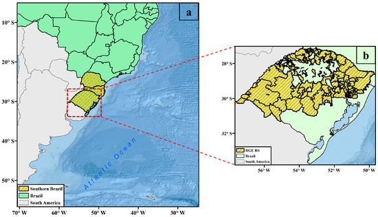
Figure 1.
(a) South Brazil (hatched) and the South Atlantic Ocean and (b) the RGE concession area situated within the state of Rio Grande do Sul, located in southern Brazil.
2.2. Data
In this subsection, the data used in this study are presented.
2.2.1. ERA5 Reanalysis
The term ERA5 reanalysis [19] stands for Fifth Generation of Atmospheric Reanalysis produced by the European Centre for Medium-Range Weather Forecasts (ECMWF). This dataset combines vast amounts of historical observations into global estimates using a sophisticated model and a data assimilation system. This reanalysis provides a diverse set of variables that are spatially comprehensive and dynamically consistent regarding global atmospheric circulation. The ERA5 reanalysis encompasses a historical series from 1940 to the present day, with a spatial–temporal resolution of approximately 27 km and an hourly output.
We used hourly atmospheric and ocean data (Table 1) from 29 June to 3 July 2020 in order to characterize the EC at different atmospheric levels.

Table 1.
Atmospheric and ocean data from ERA5 used in this study.
2.2.2. Multi-Source Weighted-Ensemble Precipitation
Multi-Source Weighted-Ensemble Precipitation (MSWEP) is a global precipitation dataset available at a temporal frequency of 3 h, with a spatial resolution of 0.1° [20]. This product combines high-quality data sources available based on time scale and location: station data, satellite data, and climate reanalysis data. This data option is used for regions where there is limited availability of weather station data (in situ measurements) to achieve enhanced spatial and temporal data resolution and to contribute to a more comprehensive analysis. MSWEP data are available from 1979 to the present (virtually in real time) at 3-hourly, daily, and monthly frequencies.
Daily data from 29 June to 3 July 2020 were utilized to assess the highest rainfall accumulations associated with the EC.
2.2.3. Power Outages
Power outages that occurred within the RGE concession area were analyzed and categorized by electrical clusters. According to [21], electrical clusters of consumer units are defined by Distribution Substations (SED, in Portuguese) and encompass the medium-voltage networks downstream from the SED.
The power outage data for each electrical cluster were provided from the emergency report. The purpose of this report was to outline the procedures adopted for classifying outages during emergencies prompted by extreme weather events that impacted the energy distributor’s concession area. This report includes details such as the dates of the start and end of an event, the affected municipalities, damages to the power grid, and the distributor’s response to the situation.
2.3. EC Definition
According to [2], the concept of ECs was initially introduced by Tor Bergeron, who defined a rapid intensification of extratropical cyclones as a pressure drop of 24 hPa within 24 h. This intensification rate is referred to as the Bergeron number. Tor Bergeron primarily focused on cyclones at Bergen latitude (~60° N). Therefore, Sanders and Gyakum (1980) adjusted Tor Bergeron’s ECs definition for any latitude (φ). This is based on the value of the normalized deepening rate (NDR) of the central surface pressure [2], measured in Bergeron units (B), and is expressed as follows:
where represents the deepening rate of the mean sea level pressure over 24 h, sin(φ) is the sine of the cyclone’s latitude, and sin(60°) is the sine of the reference latitude of a cyclone.
Ref. [6] also suggested a classification of ECs in three categories: weak (1.0 ≤ NDR < 1.3), moderate (1.3 ≤ NDR < 1.8), and strong (NDR ≥ 1.8). This classification has been used in studies for the two hemispheres [5], including in the southwest South Atlantic Ocean [4,17].
These ECs are also commonly called cyclonic bombs. The mean sea level pressure is extracted from the cyclone’s center, and the rates of intensification are computed for each time step of cyclone centers that fall within the same trajectory in a 24 h interval.
To better understand the possible causes behind the formation of the EC, we analyzed the synoptic environment favoring its explosive genesis, focusing on the transportation of temperature and specific humidity in the lower troposphere, ascending motions, sea surface temperature anomalies, the jet stream, and the baroclinicity of the system, during the period from 12Z 29 June to 12Z on 2 July 2020.
3. Results
This section is divided into three subsections describing the event through satellite images, the atmosphere and ocean conditions, and the impacts on the power supply.
3.1. Satellite Imageries
The rapidly intensifying extratropical cyclone was classified as EC. Figure 2 presents a satellite image from GOES16 in channel 13 (infrared), showing the cyclone and the associated cold front affecting the southern region of Brazil. The satellite image indicates the brightness temperature, with the lowest temperatures corresponding to greater vertical cloud extension and a higher potential for causing severe storms, as shown over the ocean.
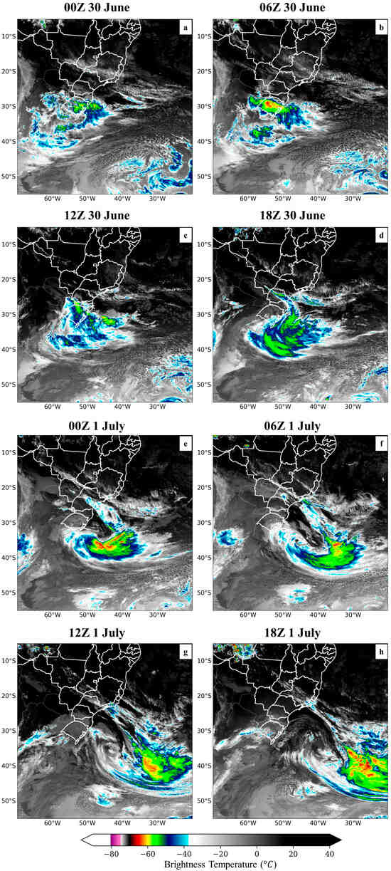
Figure 2.
Satellite imageries from GOES16 (CH13) during the development of the EC to: (a) 00Z 30 June 2020, (b) 06Z 30 June 2020, (c) 12Z 30 June 2020, (d) 18Z 30 June 2020, (e) 00Z 1 July 2020, (f) 06Z 1 July 2020, (g) 12Z 1 July 2020 and, (h) 18Z 1 July 2020.
Between 00Z and 12Z on 30 June (Figure 2a–c), during the period of cyclogenesis, a low brightness temperature was observed, indicating the presence of deep convective clouds with the potential to cause severe weather. From 18Z on 30 June (Figure 2d), cloudiness began to organize in a frontal band over the southern region of Brazil. Between 00Z and 06Z on 1 July (Figure 2e,f), the characteristic rotation of the cyclone and the associated cold front became evident, indicating a mature stage of the cyclone. Between 12Z and 18Z on 1 July (Figure 2g,h), the cyclone initiated the occlusion and decaying process, which indicated a weakening of the system.
3.2. Atmospheric and Oceanic Conditions
- Mean Sea Level Pressure and 10 m winds
From 00Z to 12Z on 29 June (Figure 3), winds were weak over the continent, and their speeds did not exceed 8 m/s.
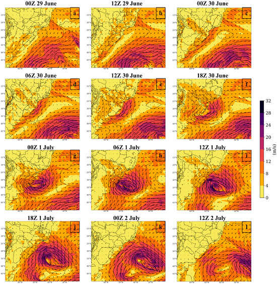
Figure 3.
Mean sea level pressure (hPa; isobars), 10 m wind intensity (m/s; shaded), and direction (vectors) to: (a) 00Z 29 June 2020, (b) 12Z 29 June 2020, (c) 00Z 30 June 2020, (d) 06Z 30 June 2020, (e) 12Z 30 June 2020, (f) 18Z 30 June 2020, (g) 00Z 1 July 2020, (h) 06Z 1 July 2020, (i) 12Z 1 July 2020, (j) 18Z 1 July 2020, (k) 00Z 2 July 2020 and, (l) 12Z 2 July 2020.
At 00Z on 30 June (Figure 3c), a low-pressure center of 1004 hPa formed between Paraguay and Argentina, approximately at latitude 23° S and longitude 62° W. In this area, wind speeds peaked at values between 4 and 12 m/s. Notably, the winds strengthened and blew parallel to the coastlines of South and Southeast Brazil, achieving magnitudes of up to 12 m/s. Wind strengthening was attributed to the strong pressure gradient between the cyclone evolving over the land and the anticyclone prevailing over the Atlantic Ocean, centered around latitude 28° S and longitude 36° W, with a pressure center of 1024 hPa.
At 06Z (Figure 3d), the cyclone began to become elongated toward the ocean, and the strongest winds blew parallel to the coast of southern Brazil, with intensities ranging from 12 to 16 m/s. At 12Z (Figure 3e), the cyclone reached the ocean and registered a pressure center of about 1004 hPa for the first time. Furthermore, the coastal winds continued to escalate, with speeds peaking at values between 16 and 20 m/s.
At 18Z (Figure 3f), at lower levels, the cyclone continued moving toward the ocean; at mid levels, the cyclonic circulation intensified, and at the surface, the low pressure dropped to 1000 hPa. The winds intensified over southern Brazil, showing maximum speeds from 8 to 12 m/s, while over the ocean in the eastern sector of the cyclone, the winds reached 20 m/s.
Ref. [10] delve into the attributes of cyclones that develop from 24° S to 36° S and from 50° W to 70° W. These cyclones originate over land but promptly move eastwards and reach the ocean due to South America’s narrow continent land at these latitudes. Consequently, these cyclones often reach oceanic areas from 12 to 24 h after their genesis, where surface fluxes can be large. The elongated contour of the low-pressure area observed during the genesis phase suggests influences from thermal–orographic lows like the Northwestern Argentina Low [22] and the Chaco Low [23].
At 00Z on 1 July (Figure 3g), the cyclone center recorded a pressure of 988 hPa, at around 34° S and 48° W, over the ocean. This low-pressure center corresponded to a 16 hPa pressure drop within 6 h. The wind intensity remained strong, attaining peak speeds of 24 m/s over the ocean. At 06Z (Figure 3h), the cyclone deepened further, marking a central pressure of 980 hPa. At 12Z (Figure 3i), the cyclone’s central pressure descended to 976 hPa, with winds of up to 28 m/s. At 18Z (Figure 3j), the system maintained its strength and continued its eastward trajectory.
At 00Z on 2 July (Figure 3k), the cyclone initiated a gradual weakening process. Finally, at 12Z (Figure 3l), the study area no longer experienced significant impacts from the cyclone.
The pressure change from 00Z on 30 June to 00Z on 2 July is shown in Figure 4. A pressure drops of 34 hPa in 24 h was recorded, starting at 14Z on June 30, with 1003 hPa, and ending at 13Z on 1 July, with 969 hPa. Thus, from Equation (1), the NDR was approximately 2 Bergeron. Therefore, the system was classified as a strong EC [2].
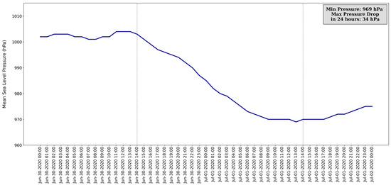
Figure 4.
Time series of mean sea level pressure variations following the cyclone’s center from 00Z on 30 June to 00Z on 2 July.
- 2.
- 850 hPa specific humidity and vertical motion
At 00Z on 29 June (Figure 5a), an intense moisture transportation was observed over Paraguay, with isolated areas of upward motion. At 12Z (Figure 5b), the transport of moisture increased, originating from the Amazon area toward Argentina and southern Brazil. This convergence of moist air at lower levels enhanced the upward motion at mid levels.
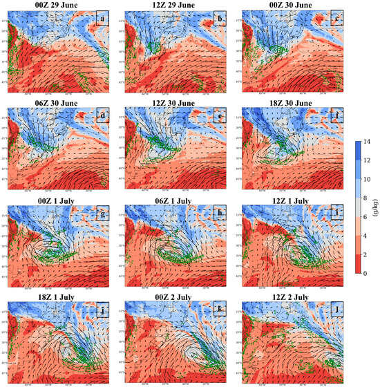
Figure 5.
Mean sea level pressure (gray contours every 4 hPa), 850 hPa specific humidity (g/kg, shaded) and winds (vectors), and 500 hPa upward motion (green contours every 10−1 Pa/s) to: (a) 00Z 29 June 2020, (b) 12Z 29 June 2020, (c) 00Z 30 June 2020, (d) 06Z 30 June 2020, (e) 12Z 30 June 2020, (f) 18Z 30 June 2020, (g) 00Z 1 July 2020, (h) 06Z 1 July 2020, (i) 12Z 1 July 2020, (j) 18Z 1 July 2020, (k) 00Z 2 July 2020 and, (l) 12Z 2 July 2020.
At 00Z on 30 June (Figure 5c), moisture transportation strengthened, particularly over the Rio Grande do Sul state. This transportation contributed to increasing the atmospheric instability. By 06Z (Figure 5d), the extension of the surface low-pressure system toward the ocean became evident. In this region, a strong horizontal moisture gradient and upward motion marked the front. By 12Z (Figure 5e), the frontal wave had the cold front section positioned over the land and the warm front section over the ocean. The cold front section showed a more intense upward motion and a larger moister area compared to its surroundings. At 18Z (Figure 5f), the contrast between the air masses became more pronounced over the land, as the strong moisture transport towards the cyclone’s core persisted, aiding in its intensification.
At 00Z on 1 July (Figure 5g), the cyclone initiated the occlusion process. Notably, intense upward motion was observed over the oceanic cyclone system. From 06Z (Figure 5h) onwards, a more pronounced southerly transportation of drier air was observed toward southern Brazil. Meanwhile, the low-pressure center continued to deepen over the ocean, accompanied by strong upward motion, particularly in its southern sector. Finally, from 00Z to 12Z on 1 July (Figure 5i,j), the cyclone attained its lowest pressure value, with a pressure drop of 34 hPa within 24 h. At this stage, there was no longer a distinct contrast in moisture content between the cyclone’s core and its surroundings.
Between 00Z and 12Z on 2 July (Figure 5k,l), the cyclone’s eastward movement implied a reduced impact on the local weather conditions over land. Nevertheless, the upward motion persisted in southern Brazil.
- 3.
- 850 hPa temperature transportation and 500 hPa geopotential height
Between 00Z and 12Z on 29 June (Figure 6a,b), anomalous warm air was advected from the Amazon region, through central Brazil, toward southern Brazil.
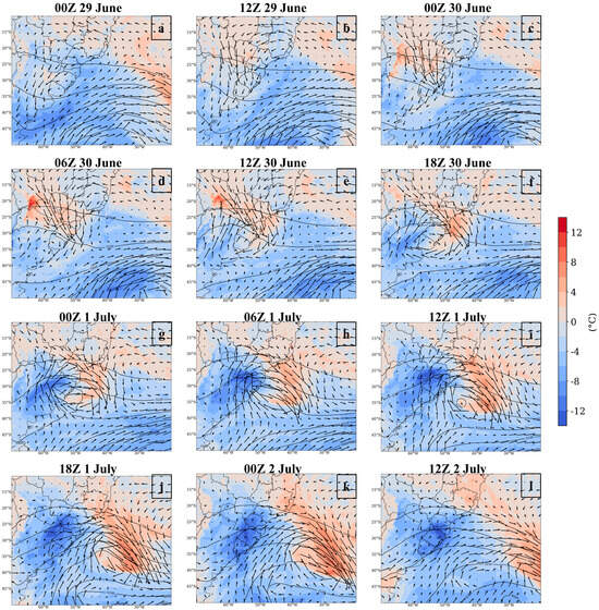
Figure 6.
The images show 850 hPa temperature transportation (°C; shaded) and winds (vectors), and 500 hPa geopotential height (m; isolines) to: (a) 00Z 29 June 2020, (b) 12Z 29 June 2020, (c) 00Z 30 June 2020, (d) 06Z 30 June 2020, (e) 12Z 30 June 2020, (f) 18Z 30 June 2020, (g) 00Z 1 July 2020, (h) 06Z 1 July 2020, (i) 12Z 1 July 2020, (j) 18Z 1 July 2020, (k) 00Z 2 July 2020 and, (l) 12Z 2 July 2020.
By 00Z on 30 June (Figure 6c), this warm air transportation increased, causing the warm and moisture-laden air (Figure 5c) to converge over the Rio Grande do Sul state, Brazil. At 06Z (Figure 6d), the transportation of anomalous warm air reached the area between Bolivia and Paraguay, around 20° S and 62° W. The warmer air contributed to a reduction in surface pressure. At the mid levels, a trough developed to the west of the surface low-pressure center.
At 12Z on 30 June (Figure 6e), the strong transportation of warm and moist air toward the coastal region of southern Brazil intensified the low-pressure system. A temperature gradient emerged between the northern and the southern sectors of the cyclone, serving as a mechanism for uplifting air and enhancing the baroclinicity of the system [17]. Moreover, the surface low pressure, coupled with vigorous upward motions, was positioned to the east of the mid-level trough, thereby increasing the system’s baroclinicity. By 18Z (Figure 6f), the horizontal temperature gradient of the cyclone intensified even further. Positive temperature anomalies of up to 8 °C were found in the region around southern Brazil and the borders of Uruguay and Argentina. These large temperature anomalies favored the intensification of the cyclone.
Between 00Z and 12Z on 1 July (Figure 6g–i), the cyclone initiated the occlusion process and acquired barotropic features, characterized by a vertically aligned structure of the trough in the lower and mid levels. This structure contained a core that exhibited warmer temperatures than its surroundings. A strong cold air transportation toward the southern region started in this interval. At 12Z (Figure 6i), the system deepened in the mid levels, with the axis of the trough positioned over the surface cyclone. The trough was approximately situated at 36° S and 45° W. At 18Z (Figure 6j), the system continued to move eastward toward the ocean.
Between 00Z and 12Z on 2 July (Figure 6k,l), the cyclone continued its eastward trajectory. In the mid levels, the long-wave trough gradually shifted alongside the system. Across southern Brazil, strong transportation of cold air was also evident.
These features agree with the findings of Gramcianinov et al. [10]. The authors emphasized a pre-genesis warm air transportation, which gained intensity due to an anticyclonic circulation northeast of the cyclone center. This circulation was potentially influenced by the South Atlantic Subtropical High, located to the east during this period. The dynamics of warm and cold transportation around the cyclone center accelerated after genesis.
- 4.
- Upper-level winds
Figure 7 illustrates the upper-level atmospheric winds, emphasizing the presence of the jet stream with speeds exceeding 40 m/s between 00Z on 29 June and 12Z on 2 July. According to [8], the intensity and frequency of ECs are associated with the location and intensity of the upper-level jet streams. The authors stated that the occurrence of ECs becomes more frequent when the jet stream increases from 45 to 75 m/s at the 300 hPa level. Furthermore, ECs are clustered on the poleward side of the jet axis, closely related to the intensification of the jet stream.
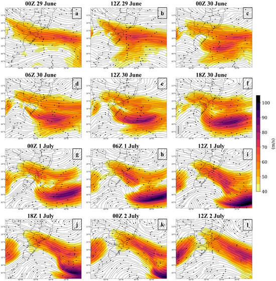
Figure 7.
The images show 200 hPa flow streamlines and speed (shaded, m/s) to: (a) 00Z 29 June 2020, (b) 12Z 29 June 2020, (c) 00Z 30 June 2020, (d) 06Z 30 June 2020, (e) 12Z 30 June 2020, (f) 18Z 30 June 2020, (g) 00Z 1 July 2020, (h) 06Z 1 July 2020, (i) 12Z 1 July 2020, (j) 18Z 1 July 2020, (k) 00Z 2 July 2020 and, (l) 12Z 2 July 2020.
Between 00Z and 12Z on 29 June (Figure 7a,b), the development of an upper-level shortwave trough was clear, with its horizontal axis positioned at approximately 26° S and 62° W. The core of the jet was positioned over the ocean, and its speeds reached 75 m/s. At 00Z on 30 June (Figure 7c), the trough further intensified over the region of Argentina. Notably, the core of the jet stream bifurcated over the ocean, each part attaining speeds of up to 75 m/s. Divergent horizontal motion at upper levels and convergent motion at lower levels contributed to a pressure reduction at the surface. Progressing between 06Z and 18Z (Figure 7d–f), the shortwave trough moved eastward fast. Moreover, the jet stream core intensified, culminating in values up to 90 m/s by 18Z.
Between 00Z to 12Z on 1 July (Figure 7g–i), the accelerated eastward trajectory of the shortwave trough consistently outpaced the mean atmospheric flow, paralleling the movement of the surface cyclone. This eastward movement of the upper-level trough contributed to reinforcing the lower-level system [10]. Concurrently, the upper-level jet stream experienced intensification due to the pronounced horizontal temperature gradient observed at lower levels. The strong upper-level jet stream strengthened the overall weather system. However, by 18Z, the system weakened as it maintained its eastward course.
Finally, spanning the interval from 00Z to 12Z on 2 July (Figure 7k,l), the jet stream weakened but was still present over the ocean, where it reinforced the surface cold front.
- 5.
- Precipitation
The transportation of warm and moist air at lower levels toward the surface trough over South Brazil favored rainfall production on 29 June (Figure 8a). On 30 June (Figure 8b), the frontal system intensified and was positioned over southern Brazil, resulting in heavy rainfall. On 1 July (Figure 8c), the system shifted eastward, and the maximum rainfall was concentrated over the ocean. Lastly, on 2 July (Figure 8d), the system moved away from the area of interest, and there was no more significant precipitation in the region.
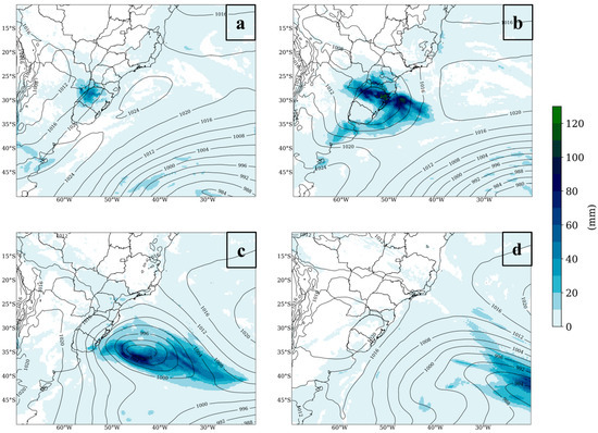
Figure 8.
Daily accumulated rainfall (shaded) and mean sea level pressure (isobars) to: (a) 29 June 2020, (b) 30 June 2020, (c) 1 July 2020 and, (d) 2 July 2020.
- 6.
- Sea Surface Temperature
Figure 9 shows the sea surface temperature anomaly for the period from 23 June to 1 July. This time window was selected to identify the pattern of the ocean conditions on the days preceding the event. The positive anomalies were particularly pronounced within the latitudes 35° S and 50° S, where the anomalies reached approximately 6° C. These warm anomalies result in strong sensible and latent heat fluxes that intensify ECs [8].
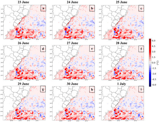
Figure 9.
Daily sea surface temperature anomalies (°C) to: (a) 23 June 2020, (b) 24 June 2020, (c) 25 June 2020, (d) 26 June 2020, (e) 27 June 2020, (f) 28 June 2020, (g) 29 June 2020, (h) 30 June 2020 and, (i) 1 July 2020.
Ref. [24] established a connection between the increased frequency of ECs in the Pacific and Atlantic Oceans and the strong sea surface temperature gradient. In the case of the analyzed EC in this study, the intense sea surface temperature gradients favored the intensification of northerly and northeasterly winds toward the warm anomalies. The pronounced anomalous warming of the ocean contributed to warming the layer of air just above this region, rendering the atmosphere unstable and resulting in a vigorous upward air motion.
- 7.
- Latent Heat Flux
Figure 10 presents the latent heat flux and sea level pressure during the period from 00Z on 29 June to 12Z on 2 July. The negative fluxes refer to heat transported from the ocean to the atmosphere, while the positive fluxes indicate transport in opposite directions.
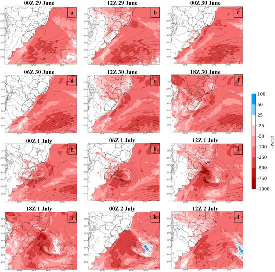
Figure 10.
Latent heat flux at the surface (W/m2) to: (a) 00Z 29 June 2020, (b) 12Z 29 June 2020, (c) 00Z 30 June 2020, (d) 06Z 30 June 2020, (e) 12Z 30 June 2020, (f) 18Z 30 June 2020, (g) 00Z 1 July 2020, (h) 06Z 1 July 2020, (i) 12Z 1 July 2020, (j) 18Z 1 July 2020, (k) 00Z 2 July 2020 and, (l) 12Z 2 July 2020.
Between 00Z on 29 June and 06Z on 30 June (Figure 10a–d), cyclogenesis occurred. At this time, some regions of positive latent heat fluxes over the continent indicated the presence of condensation.
As the cyclone formed and began to move towards the ocean, there was a strong presence of upward latent heat flux, which indicated evaporation, especially in the southern sector of the cyclone, where the sea surface temperature was warmer than the historical average temperature. Additionally, the lower levels in this region had low specific humidity. Both conditions, warmer and drier air, favored surface evaporation. The intense cyclonic winds transported moisture into the atmosphere, contributing to the system’s intensification.
During the peak intensification of the cyclone, between 06Z and 18Z on 1 July, surface-to-atmosphere heat exchanges were most pronounced. This strong surface evaporation process facilitated the ascent of warm and humid air, intensifying the upward motion and lowering the surface pressure.
From 18Z on 1 July (Figure 10j–l), there were positive latent heat fluxes over the cold front region, indicating the condensation process. In these areas, specific humidity was higher than in the surrounding areas, and precipitation was present.
3.3. Emergency in the Power Sector
We analyzed the adverse weather conditions caused by the extratropical cyclone associated with a cold front that occurred between 29 June and 3 July 2020. These conditions severely impacted the operations of energy distribution in the state of Rio Grande do Sul in the southern region of Brazil.
Electric power grids are susceptible to changes caused by weather and climate. Extratropical cyclones and cold fronts, coupled with heavy rainfall, strong gusts of wind, and electrical discharges, regularly lead to widespread and prolonged power outages. In the context of climate change, the occurrence of even more severe phenomena is projected [17], with the potential to cause significant damage to the electrical grid in the future.
For the power grid to become more resilient to these extreme events, it is essential to accurately predict the impacts that extreme weather can have on electrical systems. However, quantitatively forecasting the magnitude of high-impact weather events is challenging. Some studies, such as [25], analyzed the relationships between recent extreme events and power outages to develop a model for predicting power disruption.
During the study period, a peak of 4.3 thousand emergency occurrences was recorded, which is approximately 815% higher than the historical average. Over 800,000 consumers were affected. The first interruption occurred on 29 June, and the last interruption ended on 14 July. The impact of the severe meteorological event on the power grid hindered the swift restoration of the electrical system due to the multitude of incidents and the complexity of the restoration process. Strong wind gusts and heavy rainfall caused tree falls, blocking highways and damaging the physical infrastructure of the system.
Figure 11 displays the average of accumulated rainfall and maximum wind gusts, and Figure 12 shows the number of power interruptions that occurred during the period from 29 June to 3 July in the RGE concession area. Tree falls, atmospheric electric discharges, soil erosion, flooding, and strong winds caused power interruptions. While the entire concession area was affected by the influence of the extratropical cyclone, the eastern and northern parts experienced the highest number of interruptions. The regions most impacted by extreme rain and wind gusts were located in areas closest to the coastline, which also had the highest number of interruptions. It is important to note that all regions experienced wind gusts exceeding 50 km/h during the event. The maximum wind gusts reached values greater than 100 km/h in the areas near the coastline on 1 July. The most intense rainfall was recorded in the central-north and central-east parts of the concession area, mainly on 30 June, with values greater than 100 mm in 24 h.
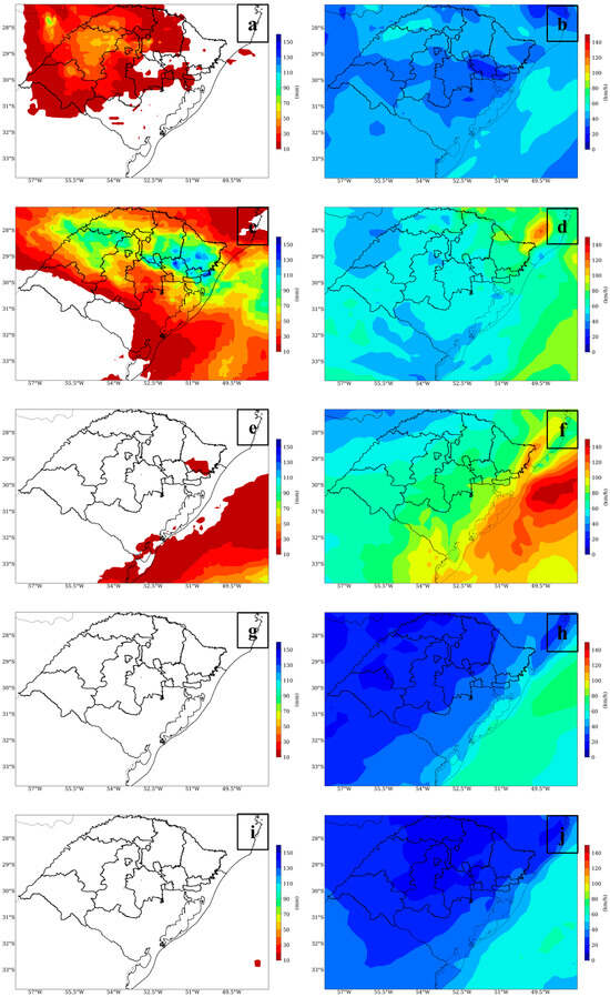
Figure 11.
Average accumulated rainfall ((a,c,e,g,i); mm) and maximum wind gusts ((b,d,f,h,j); km/h) that occurred during the period from 29 June (first line) to 3 July (the last line) in the RGE concession area in the Rio Grande do Sul state, Southern Brazil.
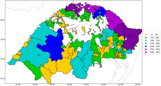
Figure 12.
Number of power interruptions that occurred during the period from 29 June to 3 July in the RGE concession area in the Rio Grande do Sul state, South Brazil.
4. Discussion
Large-scale atmospheric and oceanic conditions strongly influence the genesis and development of ECs. These systems are associated with a baroclinic environment characterized by strong horizontal temperature gradients, moisture availability, strong jet stream speeds, and air–sea interactions [3,5,8,24]. Therefore, these atmospheric and oceanic conditions were analyzed from 00Z on 29 June to 12Z on 2 July 2020 to characterize the genesis and development of the EC that occurred in that period.
Between 00Z and 12Z on 29 June, the atmospheric conditions over the continent were characterized by weak surface winds, and no surface cyclone had yet developed. However, at 12Z, the heat and moisture from the Amazon region began to be transported toward the Southern Region of Brazil. The convergence of warm and moist low-level winds fostered a vigorous upward vertical motion between Argentina and the Rio Grande do Sul state. Concurrently, the upper-level jet stream was located over Paraguay and southern Brazil, with speeds up to 60 m/s. The presence of the jet stream was induced by the meridional temperature gradient at the surface and the robust vertical wind shear, creating favorable conditions for cyclogenesis. As a consequence of these atmospheric dynamics, cloudiness and precipitation events were observed in the region.
Starting at 00Z on 30 June, a low-pressure system, with a central pressure of 1004 hPa, was positioned between Paraguay and Argentina, approximately at 23° S and 62° W. During this period, the cyclonic circulation intensified, leading to the strengthening of winds on the eastern side of the cyclone center and along the entire coastal region of southern Brazil. This intensification was associated with significant moisture transportation and heat fluxes at lower levels, resulting in moisture convergence over the Rio Grande do Sul and enhanced vertical motion. Furthermore, a trough in the jet stream was present at upper levels, aligned with the surface low-pressure area. Notably, the jet stream exhibited a bifurcation with two distinct cores over the Atlantic Ocean, with maximum speeds of up to 75 m/s.
Between 06Z and 12Z on 30 June, the cyclone was elongated towards the ocean, while the winds kept strengthening, especially along the coastal areas. Concurrently, a cold front associated with the cyclone formed over the southern region. In addition, there was a notable transportation of cold and dry air, whereas warm air transportation was evident ahead of it. In the mid levels, a trough was observed to the west of the surface low-pressure area, indicating the presence of baroclinic conditions within the system. This trough exhibited a pronounced amplification. The most intense core of the jet stream was situated east of this trough, positioned over the ocean. By 12Z, the wind speeds further intensified, reaching approximately 80 m/s at 200 hPa.
At 18Z on 30 June, the cyclone’s center positioned itself over the anomalous warm ocean for the first time. Subsequently, the cyclone experienced a rapid deepening process, intensifying significantly and moving eastward. This intensification can be attributed to the persistent transport of heat and moisture from the Amazon region towards the cyclone combined with a latent release due to the warm ocean. Additionally, the presence of the mid-level trough, slightly west of the surface low-pressure area, played a contributing role in this intensification process.
Between 00Z and 06Z on 1 July, the winds further intensified over Rio Grande do Sul due to the cyclone’s position over the ocean, near the coast. Particularly, from 06Z, there was a strong transportation of cold and dry air from the south toward the southern region, located behind the cyclone. Concurrently, an intense warm transportation occurred in the cyclone’s front. The pronounced temperature gradient associated with the cyclone amplified the potential energy available for conversion into kinetic energy, leading to further intensification of the cyclone. Between 12Z and 18Z, the cyclone reached its minimum central pressure of 969 hPa, approximately at 35° S and 45° W. This low pressure represented a remarkable pressure drop of 34 hPa within 24 h, classifying the cyclone as an EC or “bomb cyclone”. Notably, at 12Z, the cyclone exhibited a deep vertical structure, with a coherent vertical alignment from the lower to the mid levels. At 500 hPa, a low geopotential height center was evident directly above the surface low-pressure area.
At 00Z on 2 July, the intense winds persisted, particularly in regions near the coasts of the southern and southeastern areas, as well as over the ocean. By 12Z, the cyclone had moved eastward and weakened. However, in the mid levels, a long-wave trough persisted, promoting the development of surface instabilities. Meanwhile, at upper levels, the jet stream showed signs of weakening.
5. Conclusions
This study investigated the characteristics and impacts of an EC that occurred between 29 June and 3 July near the coast of southern Brazil in the South Atlantic Ocean. The investigation showed the interaction of atmospheric and oceanic heat fluxes contributing to the rapid deepening of the cyclone and its subsequent implications on the weather conditions.
The analysis of the atmospheric conditions revealed that warm air transportation and the transport of moisture facilitated the explosive cyclogenesis. The interaction of the jet stream with the cyclone’s movement played a significant role in the cyclone’s formation, development, and intensification. These factors contributed to the intensification of the cyclone, leading to a substantial drop in sea level pressure within 24 h.
The oceanic conditions, characterized by positive sea surface temperature anomalies, also played a pivotal role in fueling the cyclone’s intensification. The warm anomalies led to increased sensible and latent heat fluxes, which in turn enhanced the instability of the atmosphere and caused a strong upward vertical motion.
The impacts of the EC on the power sector were significant, with widespread power outages and disruptions in the electrical grid. This study demonstrated how extreme weather conditions associated with ECs, such as heavy rainfall and strong winds, can lead to infrastructure damage and interruptions in energy distribution.
As climate change continues to influence the weather patterns, understanding the behavior and characteristics of ECs becomes crucial for improving the resilience of the power sector and mitigating the impacts of ECs on energy distribution. This study contributes valuable insights into the mechanisms behind EC formation, the interactions between atmospheric and oceanic factors, and the resulting consequences for the power sector. By further investigating such events, researchers and policymakers can develop strategies to enhance forecasting accuracy, strengthen infrastructure, and ultimately minimize the socioeconomic impacts of extreme weather events in the future.
Author Contributions
Conceptualization, M.S. and S.C.C.; methodology, M.S. and S.C.C.; software, M.S.; validation, M.S. and S.C.C.; formal analysis, M.S., S.C.C., R.G.M. and L.C.A.; investigation, M.S., S.C.C., R.G.M. and L.C.A.; resources, M.S., S.C.C., R.G.M. and L.C.A.; data curation, M.S. and S.C.C.; writing—original draft preparation, M.S. and S.C.C.; writing—review and editing, S.C.C., R.G.M., L.C.A. and R.d.O.G.; visualization, M.S. and S.C.C.; supervision, R.G.M., L.C.A. and R.d.O.G.; project administration, R.G.M., L.C.A. and R.d.O.G.; funding acquisition, R.G.M., L.C.A. and R.d.O.G. All authors have read and agreed to the published version of the manuscript.
Funding
This study is part of the R&D PA3079—Electrical Grid Resilience Project with resources from ANEEL’s R&D program and technical and financial support from CPFL Energia (ANEEL project PD-00063-3079/2021: Resilience of Electric Networks in the Distribution Segment and the Impact of Climate Change: A Meteorological, Economic-Financial and Regulatory Analysis).
Data Availability Statement
The data presented in this study are available on request from the corresponding author.
Acknowledgments
The authors thank CPFL Energia (ANEEL project PD-00063-3079/2021). S.C. Chou thanks CNPq for the grant 312742/2021-5.
Conflicts of Interest
The authors declare no conflicts of interest.
References
- Reboita, M.S.; Gan, M.A.; da Rocha, R.P.; Ambrizzi, T. Regimes de Precipitação Na América Do Sul: Uma Revisão Bibliográfica. Rev. Bras. Meteorol. 2010, 25, 185–204. [Google Scholar] [CrossRef]
- Sanders, F.; Gyakum, J.R. Synoptic-Dynamic Climatology of the “Bomb”. Mon. Weather Rev. 1980, 108, 1589–1606. [Google Scholar] [CrossRef]
- Allen, J.T.; Pezza, A.B.; Black, M.T. Explosive Cyclogenesis: A Global Climatology Comparing Multiple Reanalyses. J. Clim. 2010, 23, 6468–6484. [Google Scholar] [CrossRef]
- Bitencourt, D.P.; Fuentes, M.V.; Cardoso, C.D.S. Climatologia de Ciclones Explosivos Para a Área Ciclogenética da América do Sul. Rev. Bras. Meteorol. 2013, 28, 43–56. [Google Scholar] [CrossRef]
- Reale, M.; Liberato, M.L.R.; Lionello, P.; Pinto, J.G.; Salon, S.; Ulbrich, S. A Global Climatology of Explosive Cyclones Using a Multi-Tracking Approach. Tellus Ser. A Dyn. Meteorol. Oceanogr. 2019, 71, 1611340. [Google Scholar] [CrossRef]
- Sanders, F. Explosive Cyclogenesis over the West-Central North Atlantic Ocean, 1981–1984. Part II. Evaluation of LFM Model Performance. Mon. Weather Rev. 1986, 114, 2207–2218. [Google Scholar] [CrossRef][Green Version]
- Seiler, C.; Zwiers, F.W. How Will Climate Change Affect Explosive Cyclones in the Extratropics of the Northern Hemisphere? Clim. Dyn. 2016, 46, 3633–3644. [Google Scholar] [CrossRef]
- Zhang, S.; Fu, G.; Lu, C.; Liu, J. Characteristics of Explosive Cyclones over the Northern Pacific. J. Appl. Meteorol. Climatol. 2017, 56, 3187–3210. [Google Scholar] [CrossRef]
- Fortunato de Faria, L.; Reboita, M.S.; Mattos, E.V.; Carvalho, V.S.B.; Martins Ribeiro, J.G.; Capucin, B.C.; Drumond, A.; Paes dos Santos, A.P. Synoptic and Mesoscale Analysis of a Severe Weather Event in Southern Brazil at the End of June 2020. Atmosphere 2023, 14, 486. [Google Scholar] [CrossRef]
- Gramcianinov, C.B.; Campos, R.M.; Guedes Soares, C.; Camargo, R. de Extreme Waves Generated by Cyclonic Winds in the Western Portion of the South Atlantic Ocean. Ocean. Eng. 2020, 213, 107745. [Google Scholar] [CrossRef]
- Ávila, A.; Justino, F.; Wilson, A.; Bromwich, D.; Amorim, M. Recent Precipitation Trends, Flash Floods and Landslides in Southern Brazil. Environ. Res. Lett. 2016, 11, 114029. [Google Scholar] [CrossRef]
- Loredo-Souza, A.M.; Lima, E.G.; Vallis, M.B.; Rocha, M.M.; Wittwer, A.R.; Oliveira, M.G.K. Downburst Related Damages in Brazilian Buildings: Are They Avoidable? J. Wind Eng. Ind. Aerodyn. 2019, 185, 33–40. [Google Scholar] [CrossRef]
- Oliveira, M.I.; Puhales, F.S.; Nascimento, E.L.; Anabor, V. Integrated Damage, Visual, Remote Sensing, and Environmental Analysis of a Strong Tornado in Southern Brazil. Atmos. Res. 2022, 274, 106188. [Google Scholar] [CrossRef]
- Pereira Filho, A.J.; Pezza, A.B.; Simmonds, I.; Lima, R.S.; Vianna, M. New Perspectives on the Synoptic and Mesoscale Structure of Hurricane Catarina. Atmos. Res. 2010, 95, 157–171. [Google Scholar] [CrossRef]
- Gobato, R.; Heidari, A. Cyclone Bomb Hits Southern Brazil in 2020. J. Atmos. Sci. Res. 2020, 3, 8–12. [Google Scholar] [CrossRef]
- De Avila, V.D.; Nunes, A.B.; Alves, R.D.C.M. Comparing Explosive Cyclogenesis Cases of Different Intensities Occurred in Southern Atlantic. An. Acad. Bras. Cienc. 2021, 93. [Google Scholar] [CrossRef] [PubMed]
- Reboita, M.S.; Crespo, N.M.; Torres, J.A.; Reale, M.; Porfírio da Rocha, R.; Giorgi, F.; Coppola, E. Future Changes in Winter Explosive Cyclones over the Southern Hemisphere Domains from the CORDEX-CORE Ensemble. Clim. Dyn. 2021, 57, 3303–3322. [Google Scholar] [CrossRef]
- Marengo, J.A.; Ambrizzi, T.; Reboita, M.S.; Costa, M.H.; Dereczynski, C.; Alves, L.M.; Cunha, A.P. Climate Variability and Change in Tropical South America. In Tropical Marine Environments of Brazil: Spatio-Temporal Heterogeneities and Responses to Climate Changes; Springer: Cham, Switzerland, 2023; pp. 15–44. [Google Scholar]
- Hersbach, H.; Bell, B.; Berrisford, P.; Hirahara, S.; Horányi, A.; Muñoz-Sabater, J.; Nicolas, J.; Peubey, C.; Radu, R.; Schepers, D.; et al. The ERA5 Global Reanalysis. Q. J. R. Meteorol. Soc. 2020, 146, 1999–2049. [Google Scholar] [CrossRef]
- Beck, H.E.; van Dijk, A.I.J.M.; Levizzani, V.; Schellekens, J.; Miralles, D.G.; Martens, B.; de Roo, A. MSWEP: 3-Hourly 0.25° Global Gridded Precipitation (1979–2015) by Merging Gauge, Satellite, and Reanalysis Data. Hydrol. Earth Syst. Sci. 2017, 21, 589–615. [Google Scholar] [CrossRef]
- ANEEL. Módulo 8—Qualidade Da Energia Elétrica. Available online: https://antigo.aneel.gov.br/documents/656827/14866914/M%C3%B3dulo8_Revisao_8/9c78cfab-a7d7-4066-b6ba-cfbda3058d19 (accessed on 19 February 2024).
- Seluchi, M.E.; Saulo, A.C.; Nicolini, M.; Satyamurty, P. The Northwestern Argentinean Low: A Study of Two Typical Events. Mon. Weather. Rev. 2003, 131, 2361–2378. [Google Scholar] [CrossRef]
- Saulo, A.C.; Seluchi, M.E.; Nicolini, M. A Case Study of a Chaco Low-Level Jet Event. Mon. Weather Rev. 2004, 132, 2669–2683. [Google Scholar] [CrossRef]
- Seiler, C.; Zwiers, F.W. How Well Do CMIP5 Climate Models Reproduce Explosive Cyclones in the Extratropics of the Northern Hemisphere? Clim. Dyn. 2016, 46, 1241–1256. [Google Scholar] [CrossRef]
- Watson, P.L.; Spaulding, A.; Koukoula, M.; Anagnostou, E. Improved Quantitative Prediction of Power Outages Caused by Extreme Weather Events. Weather Clim. Extrem. 2022, 37, 100487. [Google Scholar] [CrossRef]
Disclaimer/Publisher’s Note: The statements, opinions and data contained in all publications are solely those of the individual author(s) and contributor(s) and not of MDPI and/or the editor(s). MDPI and/or the editor(s) disclaim responsibility for any injury to people or property resulting from any ideas, methods, instructions or products referred to in the content. |
© 2024 by the authors. Licensee MDPI, Basel, Switzerland. This article is an open access article distributed under the terms and conditions of the Creative Commons Attribution (CC BY) license (https://creativecommons.org/licenses/by/4.0/).