Exploring Methods for Developing Local Climate Zones to Support Climate Research

Abstract

Meteorological and climate prediction models at the urban scale increasingly require more accurate and high-resolution data. The Local Climate Zone (LCZ) system is an initiative to standardize a classification scheme of the urban landscape, based mainly on the properties of surface structure (e.g., building, tree height, density) and surface cover (pervious vs. impervious). This approach is especially useful for studying the influence of urban morphology and fabric on the surface urban heat island (SUHI) effect and to evaluate how changes in land use and structures affect thermal regulation in the city. This article will demonstrate three different methodologies of creating LCZs: first, the World Urban Database and Access Portal Tools (WUDAPT); second, using Copernicus Urban Atlas (UA) data via a geographic information system (GIS) client directly; and third via Google Earth Engine (GEE) using Oslo, Norway as the case study. The WUDAPT and GEE methods incorporate a machine learning (random forest) procedure using Landsat 8 imagery, and offer the most precision while requiring the most time and familiarity with GIS usage and satellite imagery processing. The WUDAPT method is performed principally using multiple GIS clients and image processing tools. The GEE method is somewhat quicker to perform, with work performed entirely on Google’s sites. The UA or GIS method is performed solely via a GIS client and is a conversion of pre-existing vector data to LCZ classes via scripting. This is the quickest method of the three; however, the reclassification of the vector data determines the accuracy of the LCZs produced. Finally, as an illustration of a practical use of LCZs and to further compare the results of the three methods, we map the distribution of the temperature according to the LCZs of each method, correlating to the land surface temperature (LST) from a Landsat 8 image pertaining to a heat wave episode that occurred in Oslo in 2018. These results show, in addition to a clear LCZ-LST correspondence, that the three methods produce accurate and similar results and are all viable options.

1. Introduction

Although cities only occupy 3% of the planetary surface area, they account for more than half of the world’s population, and this figure is expected to increase to 68% by 2050 [1]. The unprecedented urbanization rates of the past decades concentrate human activity in small areas, typically resulting in an intensification of impervious surface areas (ISAs) with low albedos, which consequently increase the surface urban heat island effect (SUHI) [2]. The heat accumulation due to urbanization in addition to the global warming effect and the more frequent heat waves [3,4,5] make cities hotspots for high temperature impact and its adverse effects on a large portion of the population [6].

Designing effective mitigation strategies aiming to reduce the heat accumulation of urban areas and the impact of heat waves requires an understanding of the interactions amongst the urban landscape, geography, and the local meteorological and climatic patterns. Currently, the data gathering techniques have been greatly aided by technological advances, which permit the detailed mapping of cities required for such efforts [7], such as the automated classification of urban structures based on improved classifiers and different datasets. Various techniques, including synthetic-aperture radar (SAR) hyperspectral, thermal, and very high resolution (VHR) optical data, have been used to gather detailed data of urban surfaces and structures [8].

However, a standard methodology to characterize a city or its constituent parts, and to catalogue the properties that affect thermal variations has been lacking, which has hampered a consistent approach to developing an appraisal of the issue. Approaching any scientific research involving urban topology would require a base common nomenclature for sharing data and results, and the Local Climate Zone (LCZ) classification emerged in response [9]. The LCZ methodology, as used in this study, was developed in 2012 by I. Stewart and T. Oke, segregating cities into 17 urban land use classes based on their morphologies such as land cover, building sizes and population densities, orientations and uses, and physical, radiative, and metabolic aspects, as summarized in Figure S1 in the Supplementary Materials. This classification is the organizational basis of the WUDAPT project to classify urban topologies, whose methodology forms one of the result sets of this exercise. As defined by the project’s organizers, WUDAPT’s aims are “to acquire and make accessible coherent and consistent descriptions and information on form and function of urban morphology relevant to climate weather, and environment studies on a worldwide basis, to provide a portal with tools that extract relevant urban parameters and properties for models and for model applications at appropriate scales for various climate, weather, environment, and urban planning purposes” [10].

This standardized classification is used to characterize any city [9] and provides geo-referenced land use data for meteorological and climatological modeling at the urban scale [11]. There are presently over 370 cities that have had their LCZ scheme mapped and made publicly available (wudapt.org (accessed on 12 April 2020), lcz-generator.rub.de (accessed on 5 April 2021)). WUDAPT’s method is well documented; however, it is lengthy and requires at least two and ideally three separate GIS clients to complete. Providing additional methods to quickly generate LCZ mappings of an urban area while preserving the same quality of output generated via WUDAPT would be of benefit to climatological researchers.

The use of other methods besides WUDAPT’s to map LCZs have been explored, such as by Geletič and Lehnert, in their 2015 definition of a method based on heights and surface fractions in the Czech Republic [12]. Wang et al. (2017) [13] explored the WUDAPT and GIS methods of LCZ mapping, finding that GIS data tends to create highly accurate results due to its previous validation and provenance from real urban morphology. Zheng et al. [14] performed a large-scale study using a modified WUDAPT method adapted to the entire Greater Pearl River Delta area, reclassifying on individual cities as necessary to accommodate differing topologies and urban morphologies. Oliviera et al. devised a GIS-based method based on multiple Copernicus data sets (similarly to one of the methods of this study) for the classification of irregular and densely urbanized southern European cities [15].

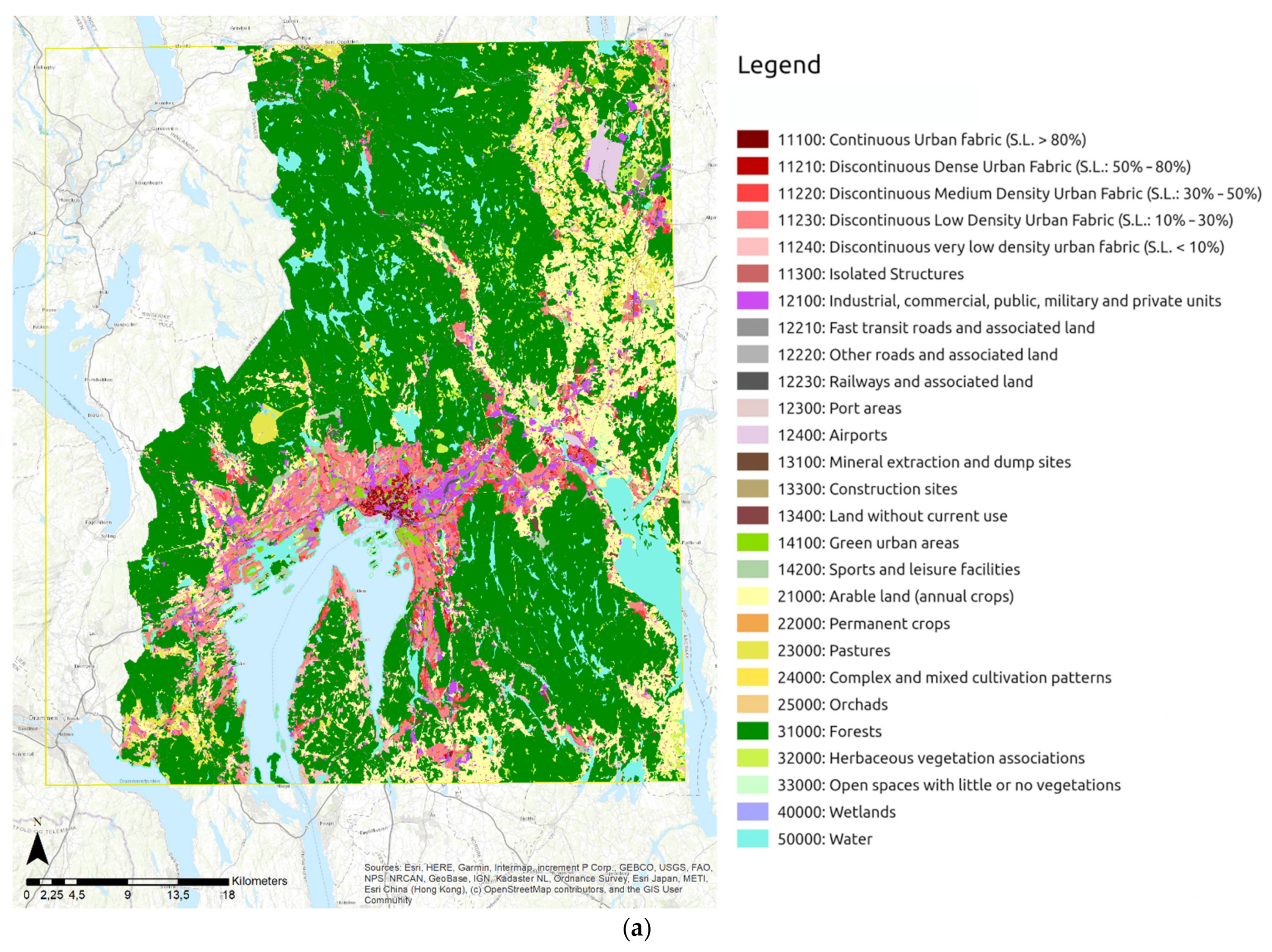
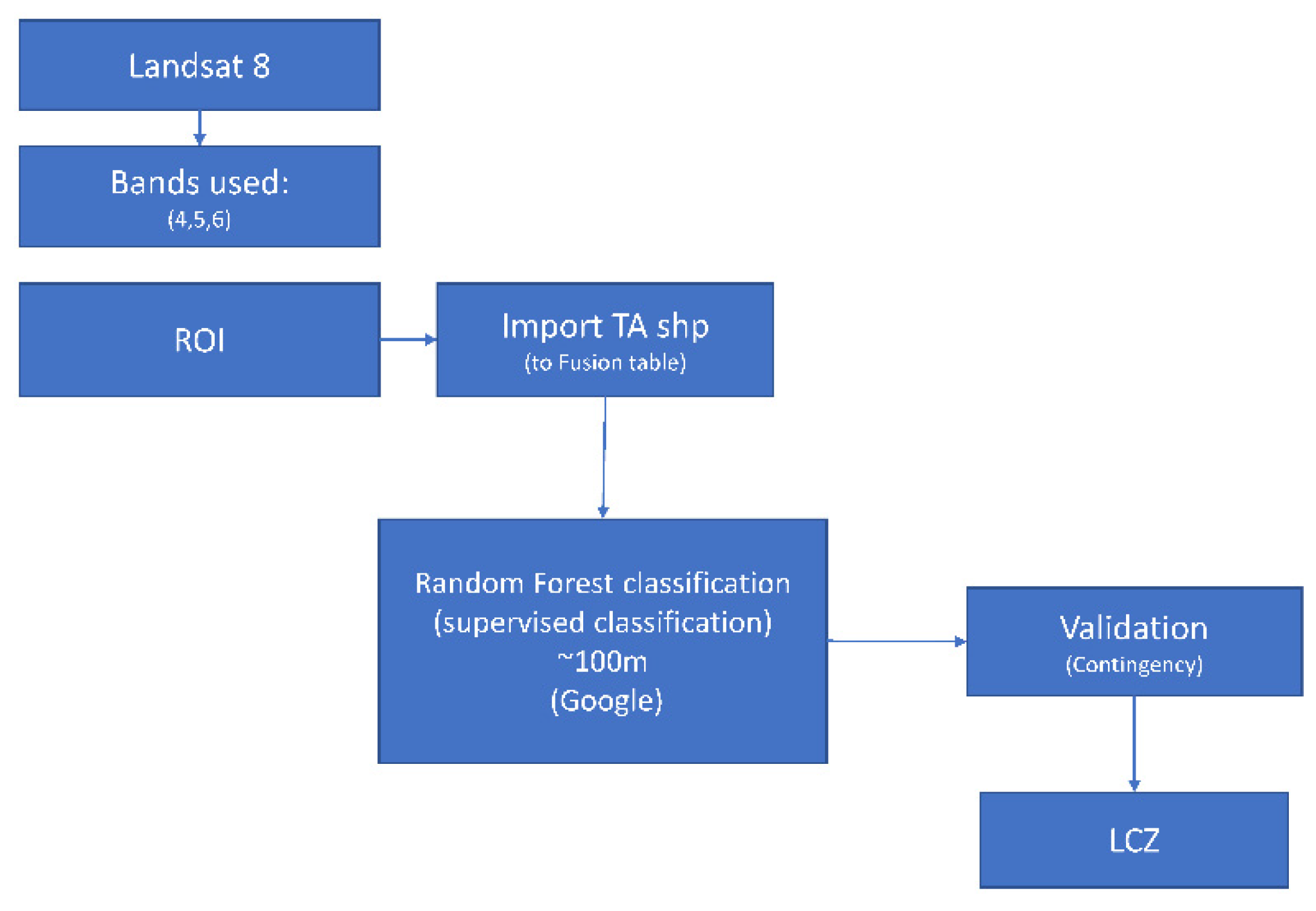
Given the need to make LCZ mapping readily available to help design mitigation and adaptation strategies to reduce the impact of climate change at the urban level, the objective of the present study is to present options to generate LCZs by demonstrating three methods for creating the LCZs of a city: (1) the WUDAPT method [10]; (2) the GIS method—reclassification of EU Urban Atlas data via a GIS client; and (3) the GEE method—Landsat 8 data interpreted through Google Earth Engine. We compare the methods in terms of the data requirements, resources required, and output quality. We illustrate the approaches by creating the LCZs of Oslo, Norway. We then validate two of the methods, the WUDAPT method via its own bespoke validation technique, and the GEE method via its own built-in functionality. The UA data has already been validated by its creators.

The three methods are then compared via a practical use of LCZs, via mapping of the distribution of the temperature according to the LCZs of each method, correlating to land surface temperature (LST) from a Landsat 8 image pertaining to a heat wave episode that occurred in Oslo in 2018. These results show, in addition to a clear LCZ-LST correspondence, that the three methods produce accurate and similar results and are all viable options. A similar study was performed by Li et al. correlating impervious surface area (ISA) with increased land surface temperatures (LSTs) [16].

2. Case Study

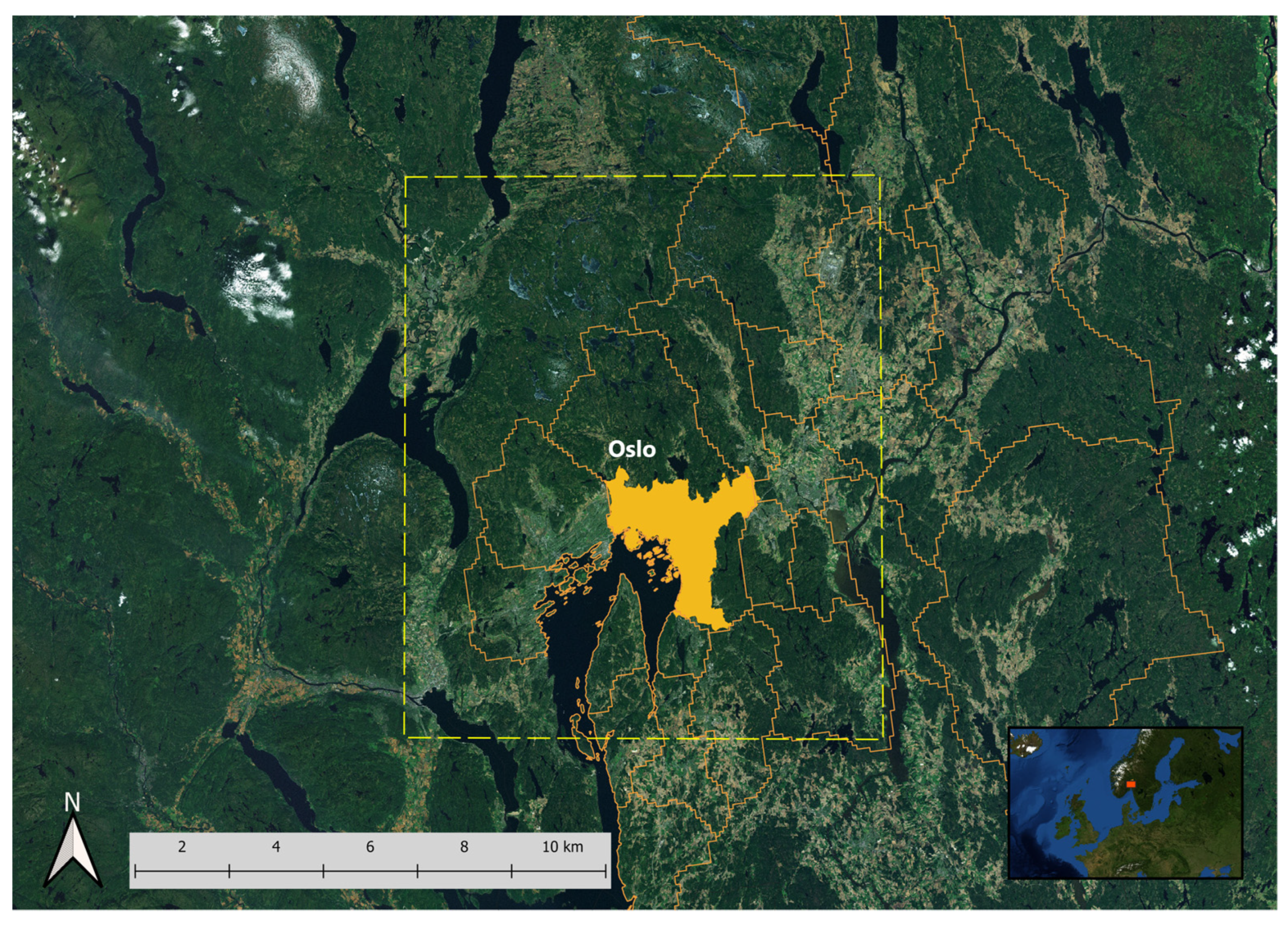
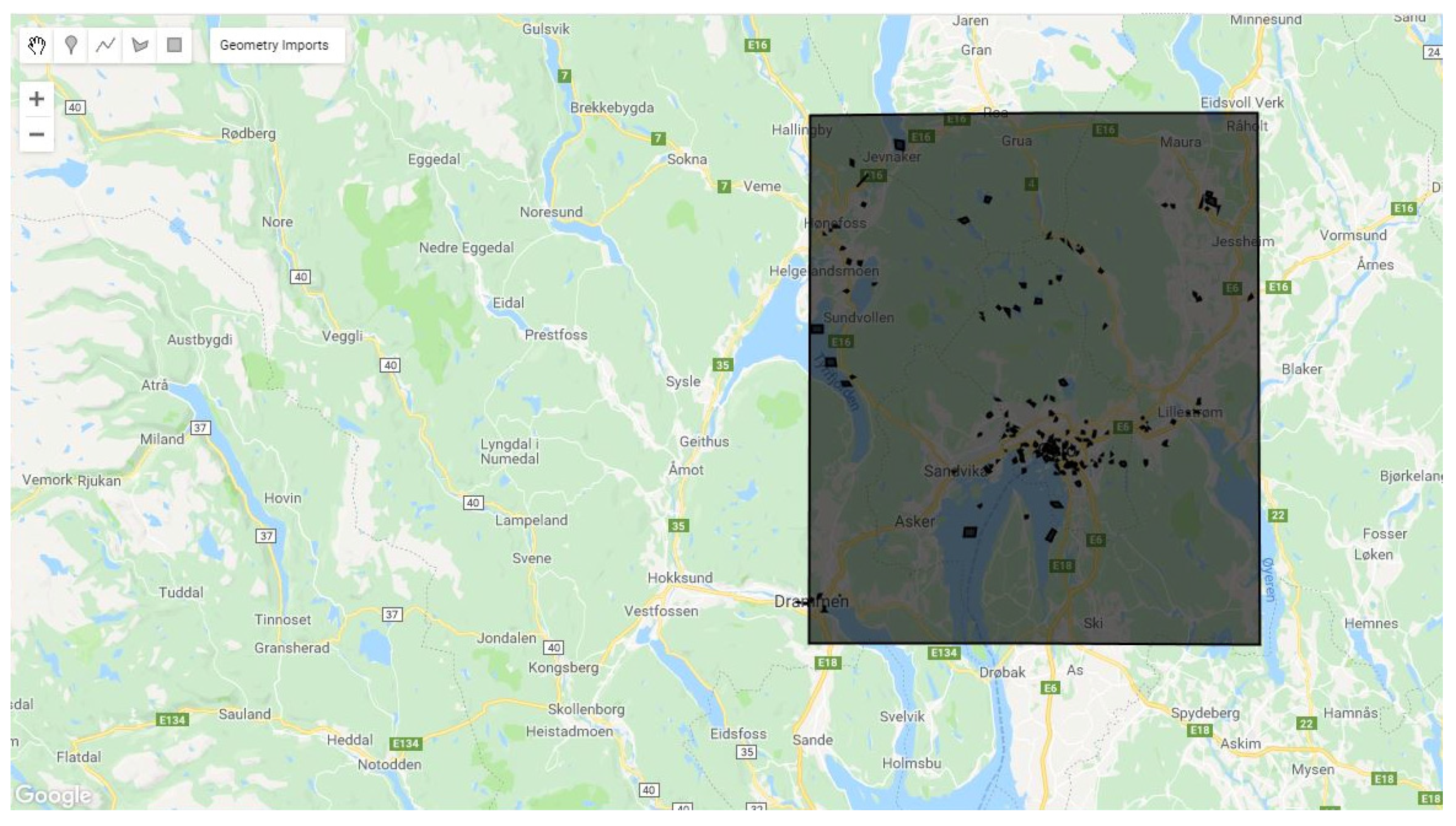
The capital of Norway is located at 59°55′ N 10°44′ E on the northern end of the Oslofjord, which gives the city access to the North Sea and is part of the Greater Oslo Region formed by 46 municipalities. The denser urbanization follows the coast in a compact conurbation, confined by hills (Figure 1). The population density of the municipality is 1580/km² [17], much lower than other European cities such as Barcelona (city limits, 15,992/km²) [18] or London (Greater—all boroughs—14,550/km²) [19], with a population of 697,010 in an area of 454 km² (Barcelona—1,664,182 in 102 km², London 9,425,622 in 1569 km²), with much of it protected wilderness. It is not a particularly old city compared to its European peers. It is low height insofar as construction, principally of 3- or 4-story buildings in the center and detached and semi-detached housing in the outskirts, with few tall (10 story or more) buildings.

Oslo has a humid continental climate, influenced by its coastal location, compared to other areas at similar northern latitudes of the city. Temperatures normally remain cool in the summer, not exceeding 20 °C, due to the proximity to the sea and the surrounding mountains. Precipitation ranges between 55 and 100 mm per year, occurring mostly during the months of summer (June–August) and autumn (September–November), which can exceed 90 mm/month. The winters can be cold with temperatures below 0 °C. The Köppen classification is Dfb (warm summer subtype/hemi boreal) and is thus much more moderate in winter than areas further inland [20]. Oslo is a wealthy city—it has a GDP per capita of 59,000 € (2016), the highest in Norway. 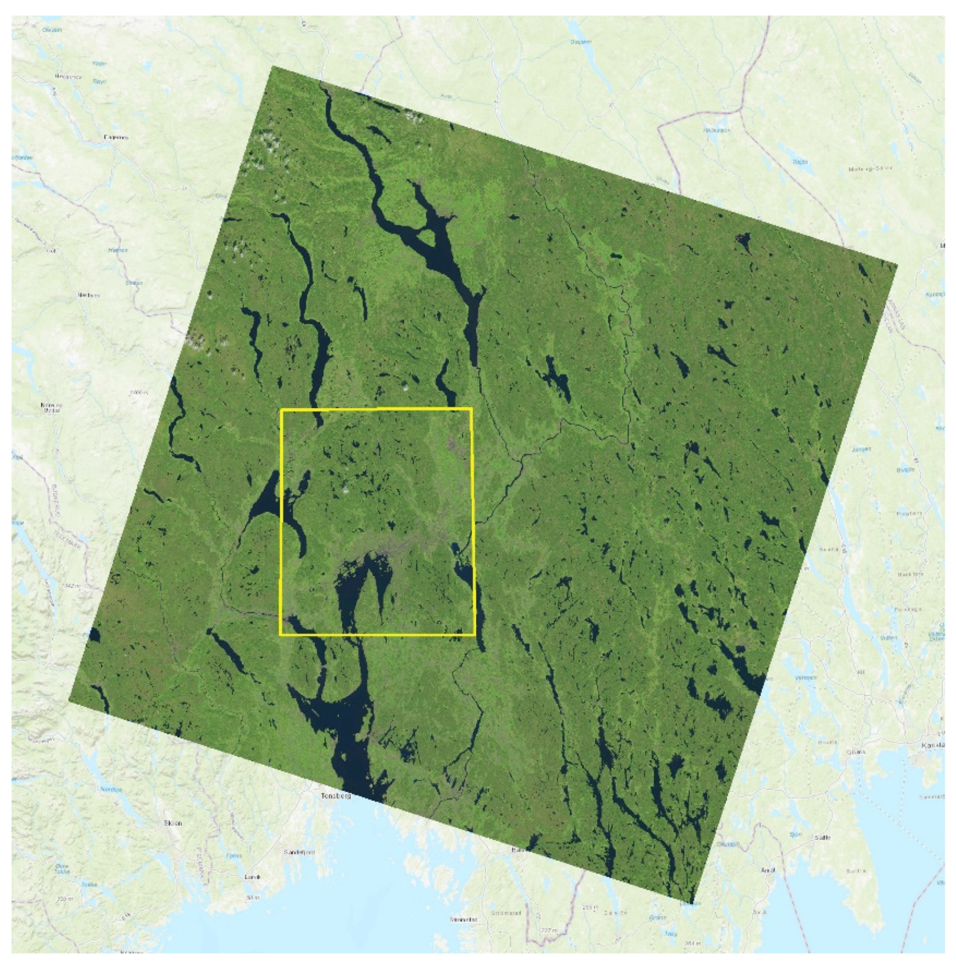Its GDP is 20% of Norway as a whole [21]. The region of interest (ROI) studied is a rectangular area encompassing the city and a large area of its surroundings, drawn to encompass as much of the urbanized metropolitan area as possible.

3. Methods

The WUDAPT and GEE methods require a satellite image to begin the process, Therefore, we used the same Landsat 8 image (Figure 2), taken on 3 July 2018. A clear image with no cloud cover is essential for LCZ exercises.

The first step of mapping the LCZs, regardless of the method, is to define the region of interest (from now on referred to as ROI). The ROI is drawn to encompass as much of the urban area as reasonably possible. It should contain a buffer around the urban area—in the case of Oslo, we used a 10-km-wide ROI as the city is compact. Norwegian municipalities tend to cover large areas while their urbanized zones tend to be small and follow the contours of valleys and inlets, not following a usual radial pattern as found in many cities on more even terrain. This results in an ROI for Oslo that has a preponderance of LCZ zone A (dense trees and forest) (see Figure 1), the most typical unaltered land state of Norway, covering roughly 60% of the ROI while roughly 12% is urbanized area. The ROI was created as a kml file using Google Earth Pro desktop software (6.0, Google, USA), as it has global coverage and provides an easy and rapid manner to define the area.

3.1. Creation of LCZ via the WUDAPT Method

The WUDAPT method is well documented [22] and we will only briefly summarize the main steps, as illustrated in Figure 3. The reader can refer to the WUDAPT documentation [23] for further and more detailed information on this method. The initial step, as with all other methods, is to create the ROI. Secondly, training areas (TAs) are drawn manually in Google Earth Pro, using visual observation of satellite imagery. The TAs are representative areas of each type of LCZ in the ROI, spaced not adjacently, of simple polygons, at least 200 m wide. Approximately 20 primary training areas and 10 test training areas are drawn, respectively. Note that the TA acronym in this study refers to the training areas as a whole (primary and test). The primary areas for the central area of the ROI are shown in Figure 4. These primary areas are the TAs that will be used to generate the LCZ mapping via the random forest classification and its later validation. The test areas are used as a separate control set for the validation of the results. The training areas are first generated as kml files, which are later transformed to shapefiles.

In parallel to creating the training areas, a Landsat 8 image covering the ROI during a moment of no cloud cover (3 July 2018) was obtained from the US Geological Survey Explorer system (https://earthexplorer.usgs.gov/ (accessed on 12 April 2020)). The satellite imagery and the training areas were combined for processing and classification using SAGA, an open-source GIS client specialized in raster image manipulation. However, other GIS software (QGIS, ArcMap) could be used if necessary. After the training areas and the satellite imagery were merged and the satellite image clipped to the area of the ROI correctly, it was necessary to resample everything to a spatial resolution of 100 m², as the Landsat 8 scene resolutions vary by the sensor used: the bands 11 and 12 (TIRS) are 100 m, the band 8 (panchromatic) is 15 m, and everything else is 30 m. We used the 100 m² resolution as a standard for the exercise. We used bands 2–7, 10 y 11 [24], skipping band 9, which helps to differentiate cirrus clouds, and band 8, which has the mentioned resolution difference.

At this point, all was ready to begin the classification/training process using the random forest machine learning method incorporated in SAGA. This was carried out by combining the satellite imagery and the training areas in the GIS and running the random forest algorithm as detailed in the WUDAPT procedure. This resulted in the classification of the image within the ROI according to the 17 LCZs categories based on the TA samples. The results were evaluated according to the k-test described in method Section 4, additional training areas added until the evaluation criteria was reached, and the classification was rerun until all zones were identified as accurately as possible.

3.2. Creation of LCZ via the Urban Atlas Method (GIS Client)

The ESA Copernicus Urban Atlas project [25] (from now on referred to as UA) provides pan-European comparable land cover and land use data for Functional Urban Areas, which can be used to create LCZs. It includes 17 urban classes with a minimum mapping unit (MMU) of 0.25 ha and 10 rural classes with MMU 1 ha (Figure S2, Supplementary Materials).

As depicted in the workflow (Figure 5), this method starts off using a vector shapefile downloaded from Copernicus (https://land.copernicus.eu/local/urban-atlas (accessed on 12 April 2020)), opened in the GIS client, and clipped to the same ROI created using the WUDAPT method in Section 3.1. The UA categories were reclassified into LCZ categories as shown in Figure S1 of the Supplementary Information, in the Esri ArcMap client, which resulted in a new vector file with the LCZs defined. Unfortunately, the UA data does not include building height information; therefore, visual observations or the use of LIDAR data are needed to accurately assign each LCZ, since the LCZ typologies depend on the building height, among other factors. In this study, we were able to extrapolate building height from Google Earth because Oslo has a very homogenous landscape of medium-height buildings.

The vector file with the newly reclassified LCZs created in the ArcMap client was converted to raster format and resampled to a 100 m resolution. The results of this exercise before and after the reclassification are shown in Figure 6a,b.

3.3. Creation of LCZ via the Google Earth Engine Method

This third method we describe to create the LCZ was performed using the Google Earth Engine via an internet browser, and the steps are summarized in Figure 7.

The first step of this method is common to the UA method: obtain Landsat 8 imagery of a clear day. This time, however, it could be used directly from the GEE software. Bands 4, 5, and 6 were used, as they are the most adequate for the application of the random forest algorithm. The software only allows the selection of three bands, differing from the WUDAPT method. This has possible later effects on the LCZ generation, as the resulting image can differ enough to affect the classification (explained further below). After the satellite imagery was selected, the ROI was added as a shapefile to the workspace (Figure 8). One band of the imagery was selected. The software allows one to perform a clipping (crop) action by drawing a rectangle over the ROI shape as shown by Figure 9a, creating a mask, which is applied to the satellite imagery, leaving an area of the Landsat 8 image within the ROI, as shown by Figure 9b in the workspace.

Once the workspace was prepared with the imagery clipped to the ROI, the shapefile containing the TAs was imported as a Google Fusion Table, which replicates the standard attribute table (*.dbf format) of a shapefile, including the geographic information. Google Fusion Tables functionality was discontinued; however, Google Earth can accept shapefile uploads (https://developers.google.com/earth-engine/guides/table_upload (accessed on 12 April 2020)) directly now. It was necessary to alter the data type of the source column (which contains the LCZ type) in the shapefile to numeric, as the software will not recognize and classify text values. Once imported as a Fusion Table, an alphanumeric identifier was given for the table, which can be referenced in the Earth Engine Explorer, by selecting the appropriate column, which has the LCZ class (derived from the TA shapefile), and assigning it to the corresponding classification (and standard LCZ color palette, shown in Figure S4 of the Supplementary Materials) previously entered in the GEE software (Figure 10).

Note that we already have the TAs created from our WUDAPT method, which are used directly. If one had not performed the WUDAPT method previously, the TAs would need to be created in Google Earth Pro following the same steps as detailed above in Section 3.1.

The Earth Engine software has the random forest functionality included, which is trained on the imported shapefile of the TAs at a resolution of 100 m², identical to the WUDAPT data. The LCZs generated from Earth Engine are shown in Figure 11 in the software’s interface upon original creation, again using the standard WUDAPT LCZ palette. The blue background color is coincidental.

4. Results

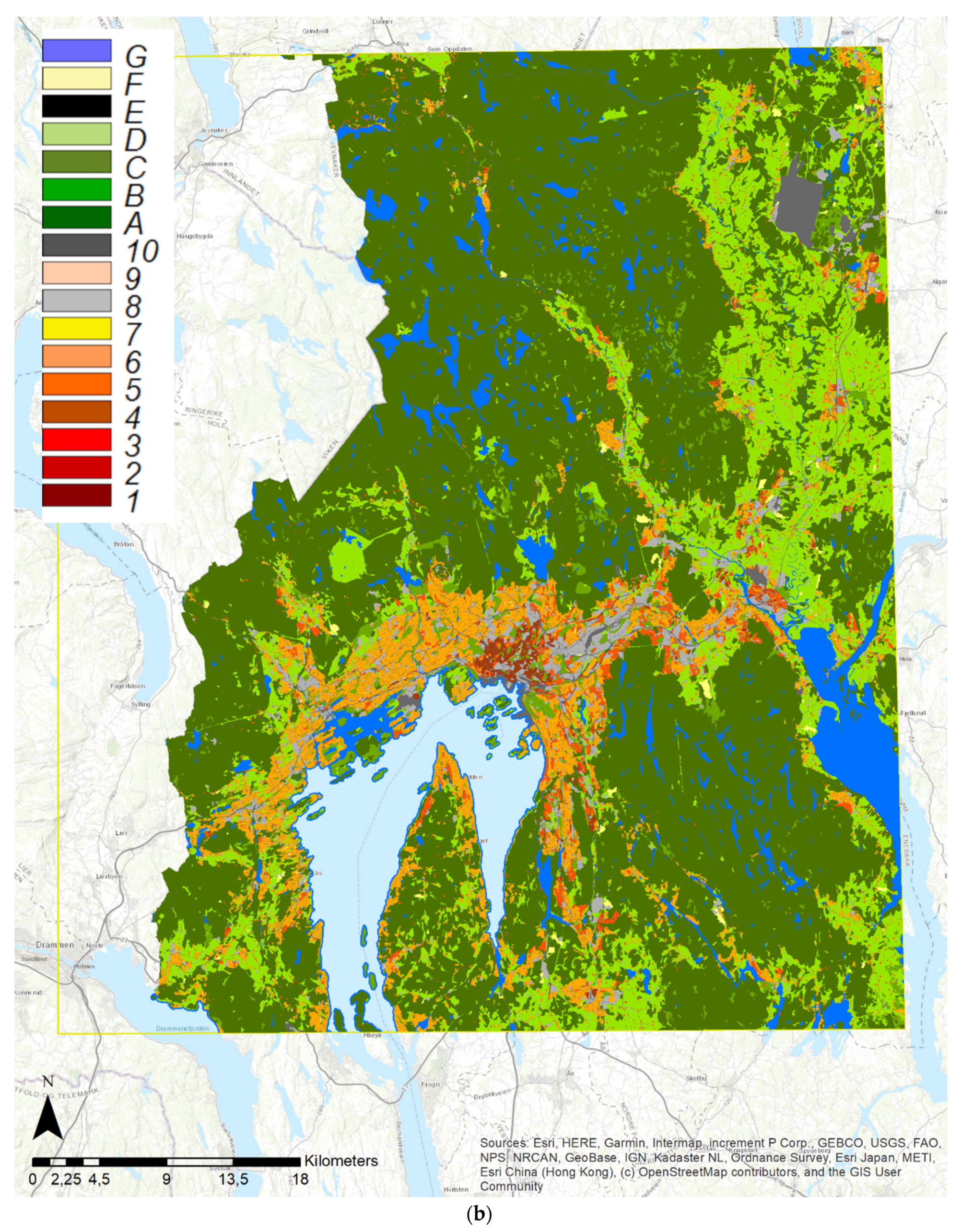
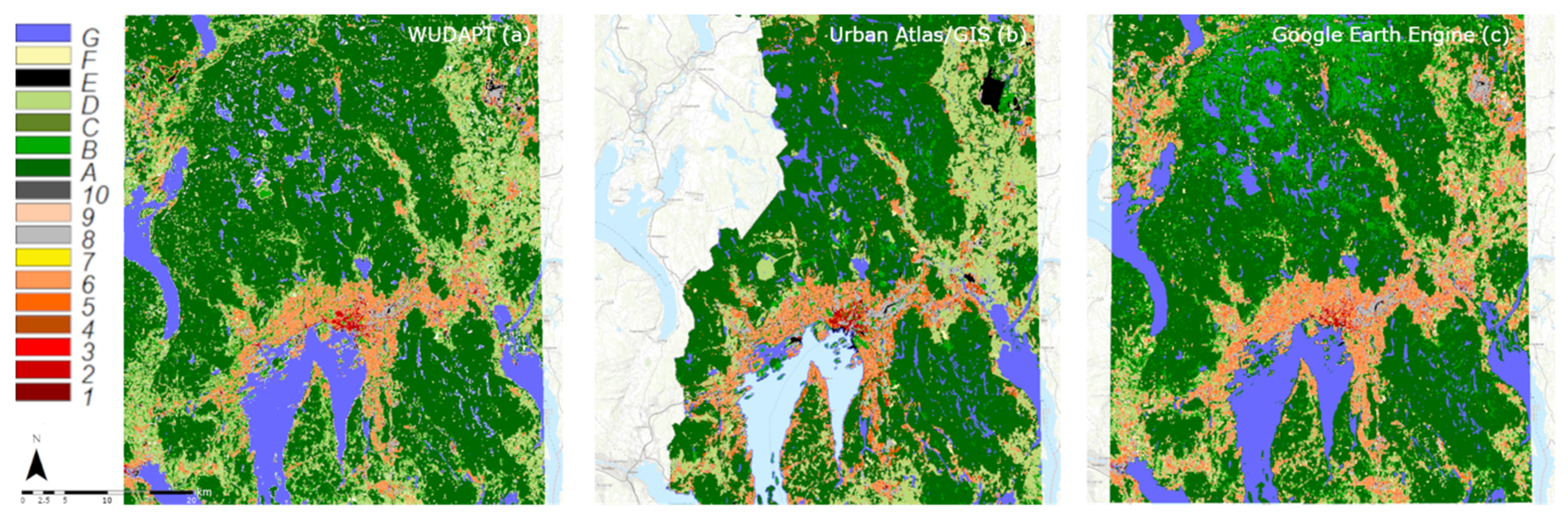
The LCZs resulting from each of the methods described are shown in Figure 12. Each method produced a usable and accurate LCZ mapping and similar results were obtained from all three.

To calculate the distribution of LCZs within the ROI and compare the results of each method, each raster layer was converted to a point layer, and the percentages of points by their LCZ values calculated. The three methodologies resulted in similar distributions of the LCZ types as shown in Figure 13. All three methods coincided, with LCZ A being the most extensive (51% to 58% of the ROI surface area) followed by LCZ B and D. The UA method and WUDAPT methods assigned more surface area to LCZ B, reflecting the grouping of forest areas in one category. In terms of the urban classes, the WUDAPT, UA, and GEE methods attributed 10, 12, and 14% of the ROI, respectively. Oslo’s urban area is mostly made up of LCZ6 (low rise, ranging from 5 to 8% of the ROI).

The difference in the distribution of LCZ types amongst the three methods could be due to several reasons. The UA/GIS data is organized differently since it is derived from a land use classification, which groups different urban topologies together. For example, government and military buildings, or airport areas, are combined as they are of a single land use. The UA data is limited to approximately two-thirds of the ROI due to political boundaries. The WUDAPT method uses nine bands from the orthophotography, whereas the GEE method is limited to three. This could result in variations in the classification by the algorithm. Another reason could be the conversion of the orthophotography from 30 to 100 m². We will further analyze these differences and reasons in the discussion section.

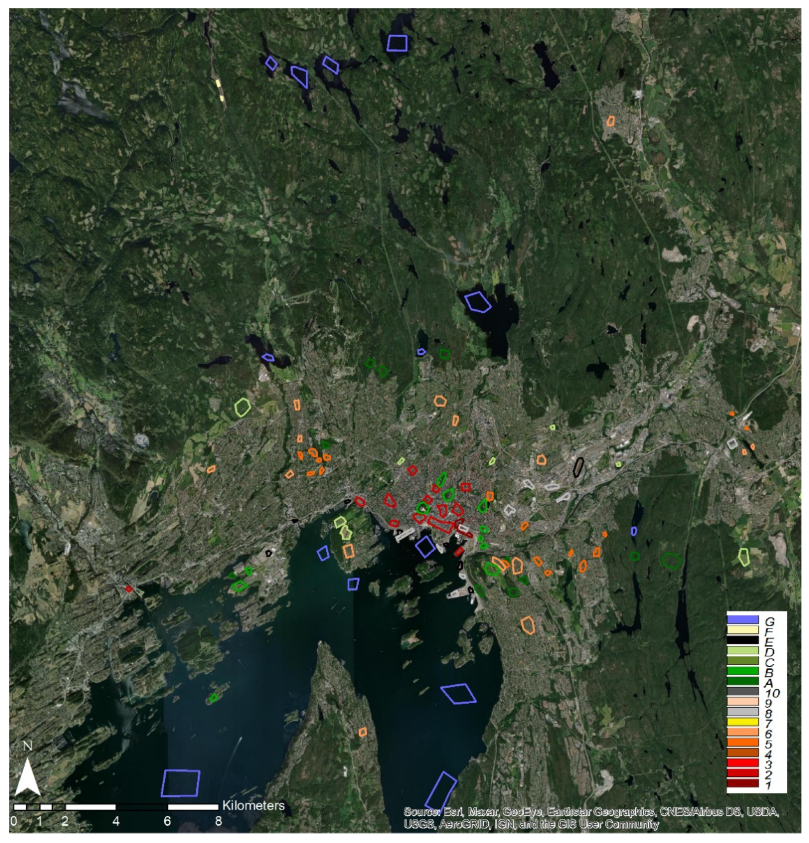
A validation of the classification was performed of the various methods. To validate the WUDAPT method and its classifiers (random forest/RF), we applied a method used by Bechtel and Daneke [8] for similar urban mapping exercises. The raster from the random forest classification was converted to a point vector layer, with each point representing a pixel from the raster, or 100 m² of the ROI. This new layer was superimposed onto the polygon layer of the training areas and clipped to match each individual TA. Then, the values of the points were determined (the LCZ values) within each training area. From this operation, we created a combined layer of points and polygons from which a confusion matrix was generated (Table S3), detailing the number of correctly and incorrectly classified points in relation to the LCZ defined by the training areas. This was carried out for both the primary and the testing training areas.

Based on this matrix, the accuracy of the random forest training and classification results was validated via a “K-test” or the Kappa coefficient, which measures the agreement and accuracy between two evaluators [26]. Kappa is calculated as:

$$k=\frac{Pr\left(a\right)-Pr\left(\mathrm{e}\right)}{1-Pr\left(\mathrm{e}\right)}$$

where Pr(a) is the actual observed agreement and Pr(e) is the chance agreement calculated in the previous step. It indicates the proportion of agreement beyond that expected by chance, that is, the achieved beyond-chance agreement as a proportion of the possible beyond-chance agreement [27]. The Kappa coefficient ranges from −1 to 1, where 1 indicates a perfect coincidence and −1 a complete difference [28] A score of one indicates complete agreement between the TAs and the classification, a score of 0 indicates no agreement, and a negative score is indicative of random results [27].

The WUDAPT validation of the classification of the primary training areas resulted in a Kappa of 0.985 and 0.869 for the test training areas; therefore, the results generated are deemed very accurate and high quality. The classifiers had slight difficulty differentiating between LCZ zones 2 and 5, and 8 and E, which are superficially similar. The resolution could cause classification errors due to some overlap along edges, as at 100 m², a large area is covered by each point/pixel, especially on an urban level.

The UA original data (the classification for the land use) was previously validated by its creators. As such, it is out of the scope of this exercise to revalidate it. The reader is pointed to https://land.copernicus.eu/user-corner/technical-library/ua-2012-validation-report (accessed on 12 April 2020) for documentation on the UA validation. Our reclassification is based upon our expert knowledge of the area and analysis of the DSM available.

Once reclassified in the GIS client, the new LCZ values were then symbolized with the standard WUDAPT legend and colors (Figure S4) and show the LCZ output for Oslo in a similar representation to the other methods.

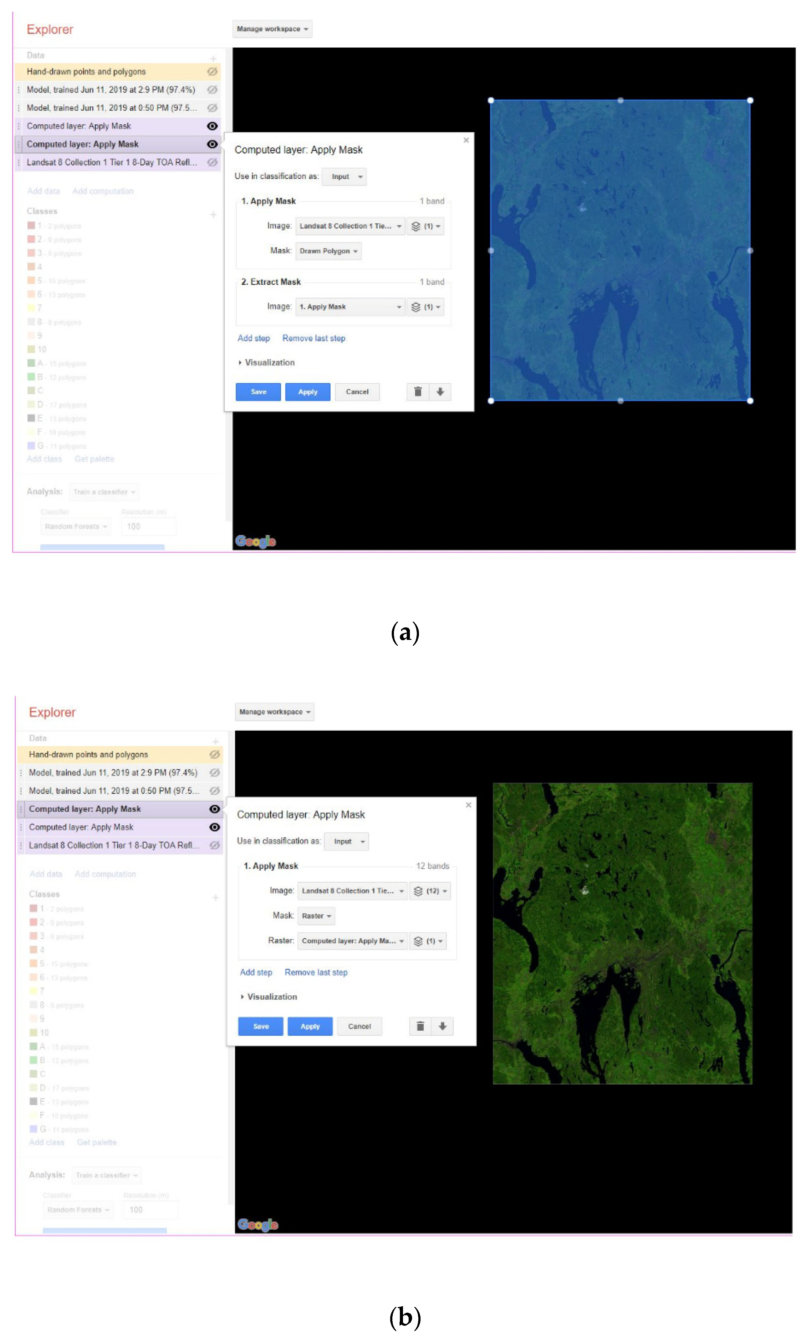
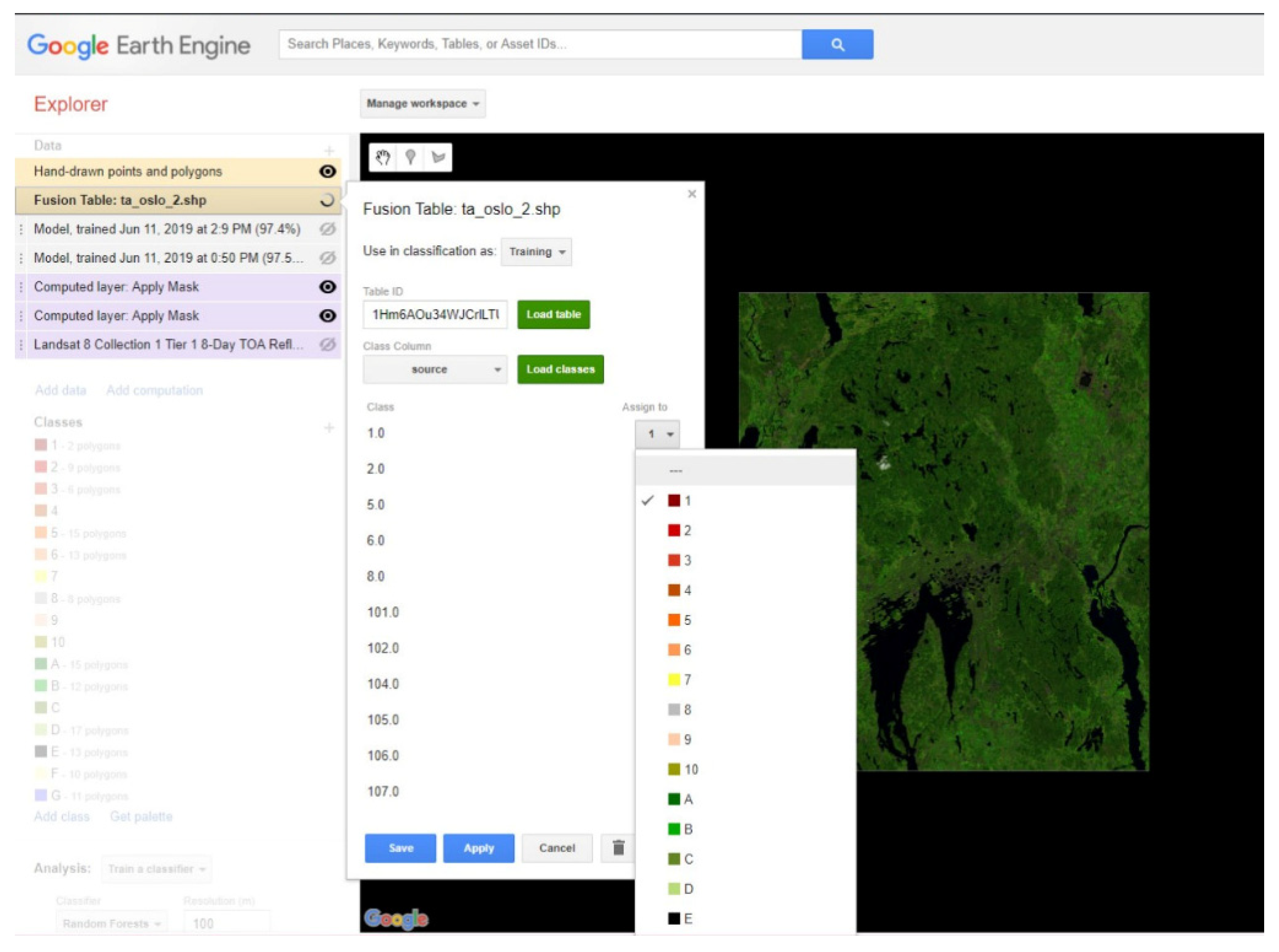
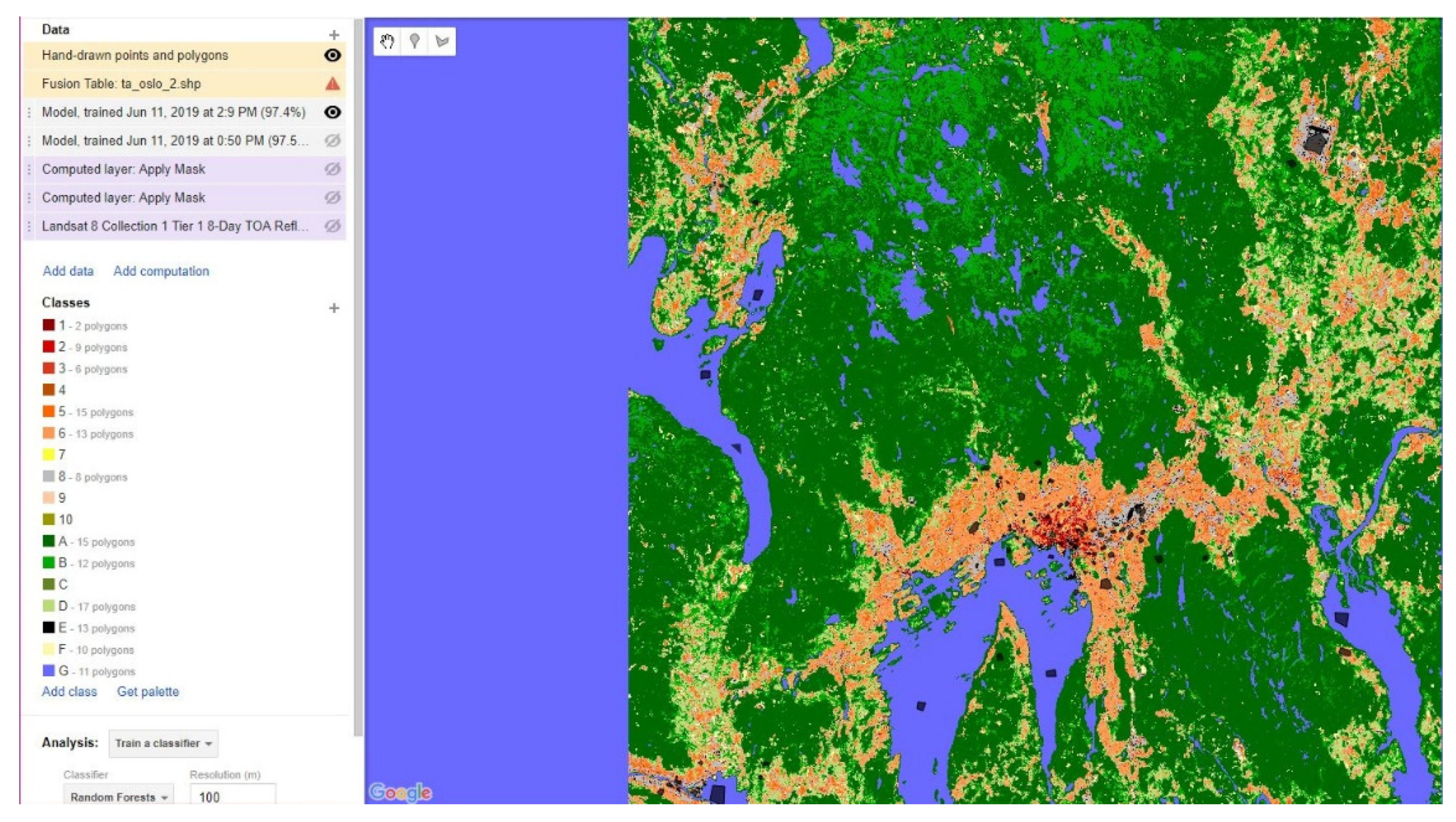
The GEE software has a built-in validation functionality (https://developers.google.com/earth-engine/guides/classification (accessed on 12 April 2020)). This validation functions in the same manner as the method described in the WUDAPT method, although it was conducted via an online interface. Once the GEE validation was performed, the software generated an attribute table (a confusion matrix) similar to that of the WUDAPT method. The confusion matrix for this method’s validation is shown in Table S3 in the Supplementary Materials.

The results of the GEE method validation were roughly as accurate as the WUDAPT method, with a Kappa of 0.974, using the same training areas, resulting in a very slight difference, which will be further analyzed in our discussion. Although the machine learning algorithms have a certain limitation, the K indexes exceed what is defined as acceptable by the WUDAPT specifications in all cases. The rural zones are not represented in the best manner, as we can observe certain confusion in different categories. The vegetated zones are confused in some cases between LCZ categories A, B, and C. Asphalted zones (type E) can be confused with industrial zones, caused by the similar nature and similarities in satellite optic channels. Category 5 and 6 can be confused due to their equal density but differing heights of structures. However, in general terms, the training areas correspond correctly, and the majority of them accurately represent the LCZ categories in both the WUDAPT and GEE methods, as seen in Tables S5–S7.

5. How Accurate Are the Various Methods of Creating the LCZ in Assessing the Influence of Urban Fabric on Surface Temperature?

As is demonstrated by the results of the comparison detailed in this section, there is a relationship between the types of materials used in urban surfaces, the height and layout of buildings, and the amount of heat that the urban surface accumulates. The ability of the LCZ method to reduce the heterogeneity of the city to 11 urban classes, each with its own material thermal properties and building layout, has made it very useful in exploring this relationship as shown by various studies [29,30,31,32]. In addition to validating the results of the three methods, we thought it would be useful for the reader to understand how accurate the various methods are in terms of assessing the influence of the urban fabric on the surface temperature. To do so, we chose a heat wave episode (as defined by Robinson [33]) that occurred in Oslo at the end of July 2018. A clear image from the Landsat 8 TIRS [34] was obtained for 30 July 2018 (Figure S8, Supplementary Materials), when temperatures reached 34.6 °C and surface temperatures up to 48 °C. To calculate LST, Landsat data of OLT/TIRS bands 4 and 5 were obtained from the USGS archives, and the method proposed by the United States Geological Survey [35] was used, as shown in the workflow illustrated in Figure S9 Supplementary Materials.

A correlation between LST and LCZ was achieved by generating near table statistics in a GIS client, based on the proximity of the points of both layers (the LCZ and the LST), using the raster image of the LST converted to points (temperature), and the points of the LCZ (classification). This procedure was repeated for each map created from the three methodologies used in the previous stages of the study. The results are shown in box/whisker format (Figure 14). A relation between LCZ and surface temperature, surface impermeability, density, and vegetation coverage was established. This result is based on partial information as the satellite imagery and land use vectors are from a directly or very close to vertical point of view; however, it gives an indicative nature of the behavior of the LCZs. The results additionally show consistency across the three methods, as expected from the validations.

Temperature Distribution According to the WUDAPT, Google Earth Engine, and Urban Atlas Methods

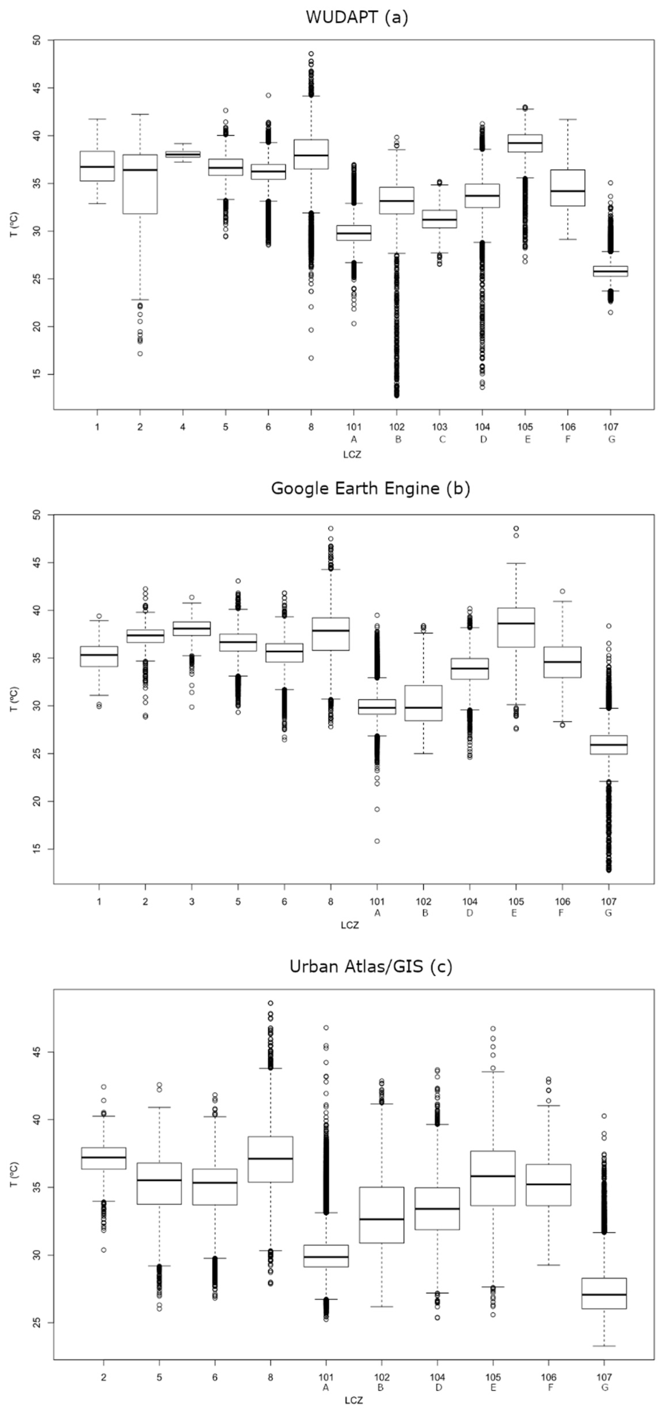
The box/whisker plot, as shown in Figure 14 shows the ranges of the temperatures within each LCZ during the heat episode. The ‘boxes’ indicate the first (Q1) and third (Q3) quartile of the dataset (25–75%, known as the interquartile range/IQR), and the ‘whiskers’ indicate each quartile to the minimum (Q1 − 1.5*IQR) or maximum (Q3 + 1.5*IQR) the minimum and maximum, with outliers indicated by single points on the lines above and below the boxes and whiskers.

A strong correlation exists between LCZ types 1 through 8 and E, which principally use materials such as concrete, tile, metal, and glass, and the highest surface temperatures. These temperatures range from 25 to 45 degrees, with outliers reaching as high as 50. Contrastingly, areas where natural surfaces predominate, such as water, soil, or vegetation—LCZ types A, B, C, D, and G—show temperatures between 25 and 42, with outliers trending lower. Note that we refer only to the surface temperature at midday in this study. Water surfaces (type G) all exhibit similar temperatures and behavior, and can be influenced by other factors (seasonal, currents, industrial) and, in turn, influence temperatures in certain zones and the area as a whole.

WUDAPT shows the general results prevalent in all three methods, with the fabricated materials (LCZ types 1–8) and type E, which includes asphalted areas but can also include rocky natural expanses as well, showing temperatures on average at least seven degrees Celsius higher during the heat episode. The lower temperature areas (LCZ types A–D and F) exhibit significant outliers, as a result of particular situations and locations of each area. This behavior is seen with type E also due to its inclusion of both manufactured and natural areas and their particular situations.

The GEE method produces results that are almost identical to the WUDAPT study, with a slight difference in the calculation of LCZ type 1, as this type is already a very small area of the ROI and slight differences in the meters included in the LCZ can affect the overall temperature recorded of the total for this type. The rest of the LCZs exhibit less outliers than in the WUDAPT method, which could be attributed to the differences in the satellite bands included in the imagery, resulting in differing classifications; however, the differences are minor.

The UA method is missing certain LCZ types because of their unavailability due to classification limitations, which has been discussed above, but the overall pattern and temperatures remain almost exactly the same: LCZ 1–8 and E show higher average temperatures than LCZs A–D and F. It is notable that LCZ E (paved and rock) is a lower temperature; however, again, this category is used as a grouping for areas that would not be necessarily included completely in this classification, for example, military or governmental facilities or airports.

The grouping of LCZs in the Urban Atlas classifications results in fewer classification categories, with wider variations in the temperatures. The original data was not intended for this use and is for general land classification purposes. Regardless, the data shows analogous temperature characteristics to those from the WUDAPT and GEE methods. The permeable and vegetated LCZs have a lower surface temperature, and the LCZs of manufactured materials tend to be higher.

Note that in comparable studies, the relation of the LCZs with temperatures were shown to be extremely similar, and the LCZs of certain types (manufactured and stone) and albedos exhibited a higher capacity to augment an SUHI characteristic [11,12].

The study of the LCZ-LST correlation reinforces the validity and reliability of the three methods applied to a practical use situation, which can be replicated for numerous urban and climatological uses. By using a clean image with no cloud cover, during the summer period, and in this case, an exceptionally high temperature event, we can characterize the behavior of the LCZs derived from the materials, colors, and physical properties (spacing, size, etc.) of them. This behavior is very close to other studies of a similar nature, such as [11,12,29,31]. Furthermore, we repeated the exercise with two more high-temperature cloud-less summer days (25 August 2020 and 28 August 2021), for which we obtained Landsat 8 images (available in Supplementary Materials, Figures S10 and S11). The resulting boxplots relating temperature with LCZ type coincide with the results obtained from the image of 20 July 2018 (available in Supplementary Materials, Figures S12 and S13). The most densely populated LCZ categories 1, 2, and 3, and industrial zone 8 and paved area E accumulate and store the most heat. Urban LCZs that are less dense, such as 5 and 6, have lower land surface temperatures, whereas the more highly vegetated or rural areas, such as A, B, C, and D, have the last heat accumulation.

6. Discussion: Advantages and Disadvantages of the Three Methods

In examining the distribution of LCZs in the ROI using the three methods (Figure 13), one can observe a similarity in the LCZ distributions amongst the three methods. The WUDAPT and GEE methods both use the same source imagery, from Landsat 8, with the only difference being the three-band limitation of the GEE software. The training areas are the same, and only minor differences in the classifications are produced in the results.

The Urban Atlas/GIS method’s results have greater differences, with the most obvious cause being that its original area does not correspond to the ROI defined for the WUDAPT and GEE studies. This is due to the political definitions of Greater Oslo limiting the area of the original UA study. The water portions of the included areas are also largely not included in the UA maps, resulting in a much lower water surface percentage compared to the other two methods. Reclassification of categories from land use to urban morphology results in ‘catch-all’ LCZs (such as type E) having a greater distribution than in the other methods. The other disadvantage is the lack of altitude data for urban structures, which would ideally be complemented with LIDAR data. A DSM via Google Earth as a reference is also available. In cities with numerous skyscrapers, LIDAR is included, with an increase in accuracy [31].

Regarding practicality and ease of use, the WUDAPT method is the most time consuming and requires a good knowledge of image processing and GIS. However, this method offers the most options to be performed manually during the process to ensure the outcome of a reliable result, due to the complete control over all stages of the process. The WUDAPT project itself has ended, but the procedures and materials are still available, and the method is in common use in the geographical and climatological fields for LCZ generation. Although, as mentioned, WUDAPT is somewhat more complex than the other two methods, presently, the continuation project, lcz-generator, allows the creation of training areas and generates the WUDAPT workflow automatically, which saves a great deal of time in the process of generating LCZ cartography. The LCZ layers for Oslo available in this project are those made from the training areas of this study. It is easier to use the Google Earth Engine method, which uses a very similar methodology to WUDAPT, and produces similar results, with increased automation and ease of use. Using the GEE method requires a familiarity with the GEE software, but it is less complicated than WUDAPT in terms of requiring only the TAs, the satellite image, and the Google Earth application.

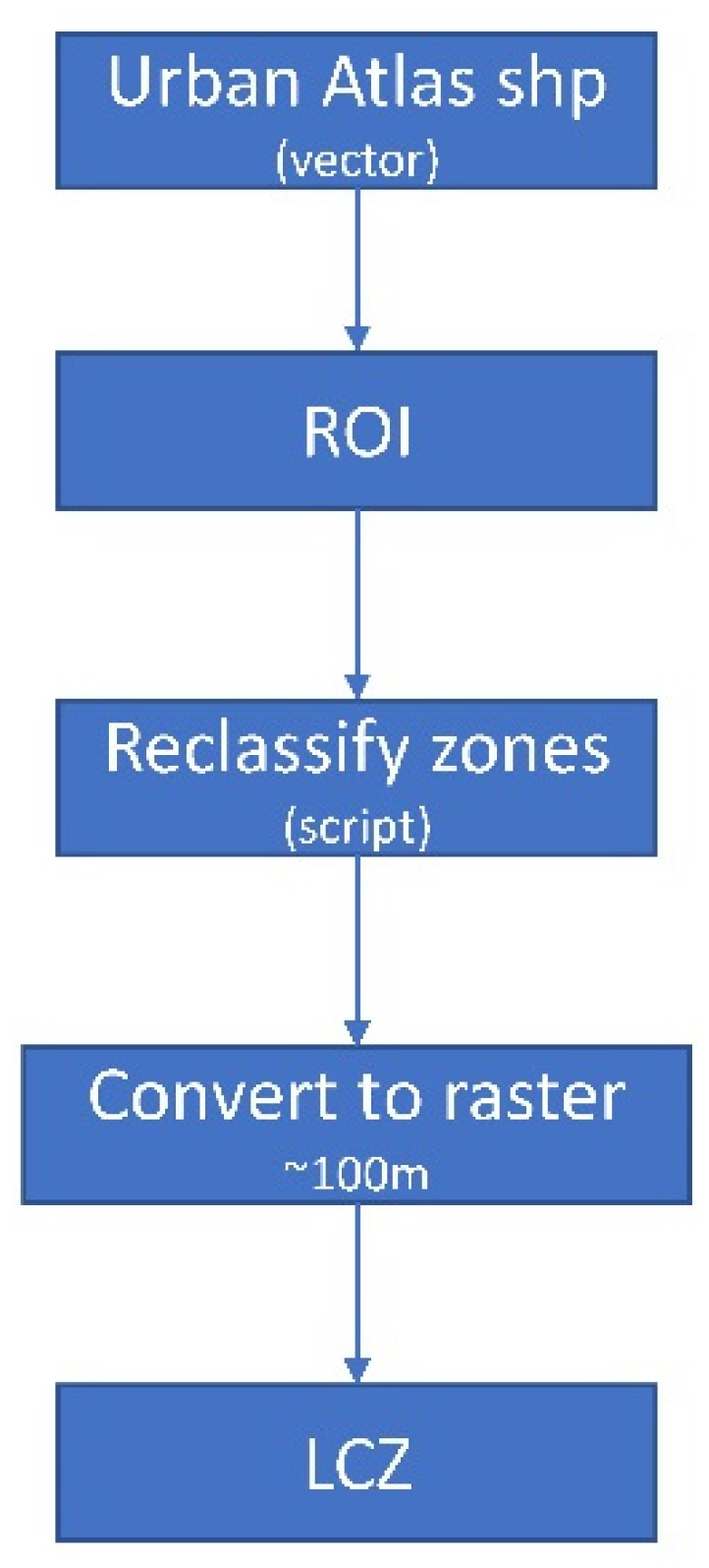
As classifications based on land use omit important details when applied to climate zone mapping, the Urban Atlas/GIS method has less precise results as the data was not originally intended for this purpose. For LCZ mapping, as per the scope of this exercise, an area’s land use is of secondary importance. This is not to say in a related study it would not be. A high-albedo, low-permeability zone such as an airport would be of interest due to the increased effects on such an LCZs’ climatological behavior from its use (pollution, heat generation, etcetera); this exercise does not provide such detail. The UA method, nonetheless, is a rapid and easy means to generate an LCZ map, with broadly reliable results. This method could also be performed with CORINE Land Cover or any similar type of vectorial land classification data, although one would only have to create an appropriate script for conversion.

The correlation between the LCZ types and the higher LST areas shows the validity of the three LCZ mapping methodologies by demonstrating the locations of areas of higher LST swings and extremes found in areas of dense urbanization and artificial materials use. This is shown in the three LCZ generation methods by the correspondence of the areas of a higher SUHI effect (temperature increases) with LCZs of artificial construction (1–8, E).

There exist discrepancies amongst the methods due to the nature of each. In both the WUDAPT and GEE methods, the same training areas and machine learning algorithm (random forest) are used on the same imagery. It is due to this reuse that the results are very close or more or less similar. On the other hand, we found differences because of the one difference at the time of the application of the algorithm: the GEE method uses only three bands of the Landsat image, and as we can see in the workflow, the WUDAPT method uses nine. For this reason and due to the nature of the random forest algorithm, we observed minor differences.

The training areas and test areas were created conscientiously and as many special areas were created on high-resolution orthophotography and a digital elevation model (DEM), Google Earth, which allowed us to determine the height of structures within LCZs.

The ROI encompasses more LCZs of a rural nature because the outlying areas of Oslo comprise forested areas and the city itself includes numerous green zones of a considerable size. However, this does not affect the precision of the algorithm. The validation results confirm that the LCZs were mapped in an optimal form and are reliable at a 100 m² resolution. In fact, although there is a higher portion of rural area within the ROI, the majority of the training areas are concentrated in the urban zones due to the difficulty in their classification, and the orientation of the LCZ mapping is for urban study. Thus, we think that the differences between the WUDAPT and GEE methods confirm that the LCZs and the training areas were designed and generated correctly.

Regarding the creation of the LCZs via the GIS/UA method, the differences are greater as the reclassification could not have been performed more accurately and we could not perform machine learning training. Regardless, the resolution of Urban Atlas is much higher than the 100 m² of the other two methods. In this aspect, one of the objectives that we desired is to refer to known methods applied in other studies similar to ours, and to compare them and evaluate the methods. There exist other studies in which methods for LCZ generation via GIS [14,15] were evaluated, and others based on machine learning (such as WUDAPT) and others that combine both (cite). Our goal was to provide references as to which methods could perform better and what limitations they might have.

The results of the validation by urban zones or the confusion are shown in Tables S5–S7. One can observe that the results are optimal in these references. A table summarizing the differences between the three methods is provided in the Supplementary Materials Table S14.

7. Conclusions

Local Climate Zones can be generated from these three different methodologies: WUDAPT, Google Earth Engine, and Urban Atlas/GIS. The three methods of LCZ generation are all accurate: the results shown in the methods’ equal placement and distribution of LCZs are similar. Each method presents certain advantages and disadvantages, which are summarized as the WUDAPT method being the most thorough and offering the most control; however, it is the most difficult and time consuming. The GEE method is similar in its approach to the WUDAPT method, using a satellite raster image and machine learning algorithm to generate LCZ mapping in a simplified manner using a web interface. The UA method is the easiest and most rapid but is derived from data fundamentally designed for uses other than urban topography and climatology. This leads to groupings of structures that are classified into completely different LCZs via the use of the other two methods. Thus, the GIS method should be performed with this caveat in mind.

It can be concluded that the three methods produce similar results and generate LCZ mappings that are more than reasonably accurate, and that these methods can be further used in applied studies. We showed that the LCZs produced can be applied to an example of the correlation between the LCZ type and surface temperatures.

This exercise can be used as a template for other cities or regions to develop LCZ mappings, with varying levels of tools and experience. It can also help other researchers to understand the advantages and limitations of each individual method, and to further refine their own individual results and improve on the methods explored here or to develop additional ones. We hope that the flexibility of being able to determine LCZs for urban areas in various ways as shown in this study will facilitate the application of land use types in urban climate simulations, urban planning, and strategies to ameliorate climate change impact.