Macroeconomic Forecasting with Factor-Augmented Adjusted Band Regression

Abstract

Previous findings indicate that the inclusion of dynamic factors obtained from a large set of predictors can improve macroeconomic forecasts. In this paper, we explore three possible further developments: (i) using automatic criteria for choosing those factors which have the greatest predictive power; (ii) using only a small subset of preselected predictors for the calculation of the factors; and (iii) utilizing frequency-domain information for the estimation of the factor models. Reanalyzing a standard macroeconomic dataset of 143 U.S. time series and using the major measures of economic activity as dependent variables, we find that (i) is not helpful, whereas focusing on the low-frequency components of the factors and disregarding the high-frequency components can actually improve the forecasting performance for some variables. In the case of the gross domestic product, a combination of (ii) and (iii) yields the best results.

1. Introduction

Factor models have become increasingly popular for the efficient extraction of information from a large number of macroeconomic variables. To investigate the forecasting performance of these models, Eickmeier and Ziegler (2008) conducted a meta-analysis of 52 studies and obtained mixed results that depended on the region, the category of the variable to be predicted, the size of the dataset, and the estimation technique. This is aggravated by the facts that it is a priori not clear how many factors should be included (Bai and Ng 2002, 2006, 2008b) and that the findings change noticeably when different sub-periods (states of the business cycle) are considered (Kim and Swanson 2014). Accordingly, many efforts have been made to improve the standard factor-augmented forecast, which is based on lagged values of the variable of interest and a small number of factors. Two approaches are of particular interest. The first approach by Bai and Ng (2008a) allows the factors to be used as predictors to depend on the variable to be predicted. As pointed out by the authors, the obvious procedure to include the factors in their natural order fails to take their predictive power into account, hence it could possibly be improved by using fewer but more informative predictors (targeted-predictors).

The second approach applies high-dimensional methods (such as pretest, Bayesian model averaging, empirical Bayes methods, or bagging) to large sets of factors. Noticing the difficulty in comparing these high-dimensional methods theoretically because of differences in the modeling assumptions and empirically because of differences in the datasets and implementations, Stock and Watson (2012) provided a general yet simple shrinkage representation that covers all these methods. Using this generalized shrinkage representation, they examined in an empirical analysis of a large macroeconomic dataset whether the shrinkage methods can outperform what is often regarded as “standard factor-augmented forecast”, i.e., the forecast based on those five factors (principal components) with the largest variances (eigenvalues). They found that this was not the case. However, factor proponents might take some small comfort in the fact that the standard forecast appeared to improve upon a simple autoregressive benchmark for a group of variables that included the major measures of economic activity (GDP, industrial production, employment, and unemployment).

In general, it is difficult to assess the significance of any further development of an existing method because the improved method is usually much more complex and depends on a larger number of tuning parameters, which increases the risk of a data-snooping bias. In the case of the standard factor-augmented forecast, Stock and Watson (2012) had to select the dataset and the investigation period, the variables to be predicted, the transformations (e.g., taking logarithms and/or differencing) to be applied to achieve stationarity, and the number of lagged values. The fact that the standard forecast improves upon an autoregressive forecast encourages not only the exploration of much more sophisticated further developments (see, e.g., Kim and Swanson 2014) but also the use of the standard forecast as a benchmark for the performance of new forecasts (see, e.g., Cheng and Hansen 2015). Clearly, the results of studies using this benchmark will be severely compromised if this improvement is not genuine. After all, what is the point of beating a bad benchmark?

There are two major goals of this paper. The first is to scrutinize the usefulness of the standard factor-augmented forecast. To that end, we reanalyze the macroeconomic dataset used by Stock and Watson (2012) with a focus on the continuous evaluation of the forecasting performance throughout the whole investigation period (1960:II–2008:IV). Our second major goal is to explore options for possible improvements. Taking up the idea that relationships between variables may exist only in certain frequency bands (Engle 1974; Hannan 1963; Reschenhofer and Chudy 2015a), we examine whether the use of frequency-domain information can improve forecasts based on factor models. We also address the central issue of how to select the factors. We may only try to determine the number of factors to be included and then just use the first factors (in their natural order) or, alternatively, find that subset of factors which has the greatest predictive power. It is only in the first case that conventional model selection criteria such as AIC and BIC are adequate. In the second case, criteria specially designed for nonnested models (Foster and George 1994; George and Foster 2000; Reschenhofer 2015; Tibshirani and Knight 1999) should be used. The third option is using a technique suitable for high-dimensional set-up, which is invariant to the ordering of predictors, e.g., LASSO (Tibshirani 1996). Finally, we exploit the possibility to reduce the set of predictors from which we then compute the factors. We first follow Bai and Ng (2008a) and use LASSO to obtain a reduced set of targeted predictors. Alternatively, we select a small set of predictors based on economic arguments.

In our rolling one-step-ahead forecasting study, we find that the inclusion of factors obtained from a large set of potential predictor series results in an improvement over a simple univariate benchmark and that the further developments proposed in this paper perform differently depending on which variables are to be predicted.

The rest of the paper is organized as follows. Section 2 discusses the models, the model-identification methods, and the forecasting techniques. In Section 3, the data as well as the data transformations are described and the empirical results are presented. Section 4 concludes.

2. Methods

2.1. Simple Linear Forecast

Let $Y_1,\dots ,Y_n$ be the time series of interest and $X_{1k},\dots ,X_{nk},k=1,\dots ,H,$ a large number of possible predictor series. Following Stock and Watson (2012), the series are first subjected to suitable transformations in order to achieve stationarity. Then, autoregressive dynamics are partialed out by regressing ${(Y_2,\dots ,Y_n)}^{\top }$ on ${(1,\dots ,1)}^{\top },$ ${(Y_1,\dots ,Y_{n-1})}^{\top },\dots ,{(Y_{-2},\dots ,Y_{n-4})}^{\top }$ and for each k, ${(X_{1k},\dots ,X_{nk})}^{\top }$ on ${(1,\dots ,1)}^{\top },$ ${(Y_1,\dots ,Y_n)}^{\top },\dots ,$ ${(Y_{-2},\dots ,Y_{n-3})}^{\top }$, where it is assumed that the observations $Y_0,Y_{-1},Y_{-2}$ are available. Denoting the estimated parameter vector of the autoregression by $\widehat{\varphi }=({\widehat{\varphi }}_0,{\widehat{\varphi }}_1,\dots ,{\widehat{\varphi }}_4)$, the residual vector by $y={(y_2,\dots ,y_n)}^{\top }$, and the residual vectors of the other regressions by $x_k={(x_{1k},\dots ,x_{nk})}^{\top }$, $k=1,\dots ,H,$ a simple forecast of $y_{n+1}$ is given by

$${\widehat{y}}_{n+1}=\sum _{k\in M}{\widehat{\beta }}_k{x}_{nk},$$

(1)

where the OLS estimates ${\widehat{\beta }}_k$ are obtained by regressing y on $x_k={(x_{1k},\dots ,x_{(n-1)k})}^{\top }$, $k\in M\subseteq \{1,\dots ,H\}$, and the associated forecast of $Y_{n+1}$ is given by

$${\widehat{Y}}_{n+1}={\widehat{\varphi }}_0+{\widehat{\varphi }}_1{Y}_n+\dots +{\widehat{\varphi }}_4{Y}_{n-3}+{\widehat{y}}_{n+1}.$$

(2)

The separate estimation of the parameters ${\varphi }_k$ and ${\beta }_j$ can be justified by orthogonality arguments.

2.2. Selecting Factors for Prediction

Model selection criteria try to balance the trade-off between the goodness-of-fit of a model and its complexity. For example, the FPE (D. Rothman in Akaike 1969; Johnson et al. 1968) uses the residual sum of squares and the number of predictors for the quantification of these conflicting objectives and selects that model which minimizes the product of the residual sum of squares and a penalty term, which increases as the number of predictors increases. The penalty term of the FPE is constructed so that the product is an unbiased estimator of the mean squared prediction error. If a predictor is included that is actually dispensable, it will still explain some random fluctuations and thereby reduce the sum of squared residuals. Clearly, this reduction will be much greater if this predictor is not fixed a priori but is found by data snooping, i.e., by trying different predictors and choosing the one which fits best. The FPE-penalty term just neutralizes the effect of the inclusion of a number h of fixed predictors; hence, its penalization will not be harsh enough if the “best” h predictors are chosen from a set of $H>h$ predictors. A data-snooping bias can only be avoided by using a penalty term that depends on both h and H. However, the two most widely used model selection criteria, namely AIC (Akaike 1998), which is asymptotically equivalent to FPE in linear regression models, and BIC (Schwarz 1978), take only the number h of actually included predictors into account. Thus, the (asymptotic) unbiasedness of AIC as well as the consistency of BIC are guaranteed only in the case of nested models where there is only one candidate model for each model dimension.

In the case of nonnested models with orthogonal predictors (e.g., principal components), unbiasedness can be achieved using a simple substitution in the multiplicative FPE-penalty term $(n+h)/(n-h)$. The number of predictors h, which coincides with the expected value of the sum of h${\chi }^2\left(1\right)$-distributed random variables, is substituted by the expected value $\zeta (h,H)$ of the sum of the h largest of H ${\chi }^2\left(1\right)$ random variables (Reschenhofer 2004). For related criteria, see George and Foster (2000); Tibshirani and Knight (1999), and, for tables of $\zeta (h,H)$, see Reschenhofer (2010). However, the resulting criterion ${\mathrm{FPE}}_{\mathrm{sub}}$ suffers from important shortcomings. Firstly, its usefulness is limited by the fact that the values of $\zeta (h,H)$ are not readily available in software packages and must be looked up in tables. Secondly, the penalty term $(n+\zeta (h,H\left)\right)/(n-\zeta (h,H\left)\right)$ may quickly become numerically unstable as h and H increase. Thirdly, the increase from $\zeta (h,H)$ to $\zeta (h+1,H)$ seems to be too small to prevent the inclusion of an unneeded predictor when there are h dominant predictors that are certain to be included. In this case, it would be more appropriate to regard the first h predictors as fixed and the next predictor as the best fitting of the remaining $H-h$ predictors rather than as the worst fitting of the best $h+1$ predictors.

Luckily, we can deal with all three issues at the same time by taking a stepwise approach (STP), according to which model dimension $h+1$ should be preferred over model dimension h if

$$\frac{n+h+\zeta (1,H-h)}{n-h-\zeta (1,H-h)}\mathrm{RSS}(h+1)<\frac{n+h}{n-h}\mathrm{RSS}\left(h\right),$$

(3)

where $\mathrm{RSS}\left(h\right)$ yields the residual sum of squares based on h predictors (see Reschenhofer et al. 2012, 2013). Here, we need only the expected value of the maximum, which can be approximated by (see (Reschenhofer 2004))

$$\widehat{\zeta }(1,H)=2log\left(H\right)-log(log\left(H\right)),$$

(4)

hence no tables are needed. Moreover, numerical problems because of small denominators occur only when h is close to n. For a related but not stepwise approach, see Foster and George (1994).

2.3. Using Factors for Prediction

A widely used method to extract h common factors from a large number of available macroeconomic and financial variables is to use the first h principal components (see (Cheng and Hansen 2015; Connor and Korajczyk 1993), (Stock and Watson 2002, 2012)), but other choices exist depending on the framework used (e.g., Forni et al. 2000, suggest using dynamic principal components for their generalized dynamic framework).

Using principal components as predictors in the spirit of Stock and Watson (2002) offers considerable advantages over using the original variables. Firstly, principal components can be ordered according to the size of the associated eigenvalues, i.e., according to the portion of variation from the original set of predictors explained by each respective component. This natural ordering of principal components allows us to think of the regression model where these components represent predictors as of a nested model. Hence, conventional criteria such as AIC and BIC become available for choosing the best model. Secondly, one can also consider nonnested setup, i.e. a classical regression setup where there is no natural ordering among the predictors. In this setup, it is often infeasible to identify the best subset of predictors. Principal components, however, are orthogonal, which makes the problem of finding the best model for each model dimension computationally tractable and therefore allows us to choose the overall best model using, e.g., stepwise procedure in Equation (3) for orthogonal predictors discussed in the previous subsection. Clearly, these advantages are purely technical and do not imply superior forecasting performance in practice.

The forecast of $y_{n+1}$ based on a subset of principal components is given by

$${\widehat{y}}_{n+1}=\sum _{k\in M}{\widehat{\delta }}_k{f}_{nk},$$

(5)

where $M\subseteq \left\{1,\dots ,K\right\}$, $K<H$, $f_k=(x_1,\dots ,x_H)v_k$ is the kth principal component with $v_k$ denoting the eigenvector associated with the kth largest eigenvalue of the sample covariance matrix of the (standardized) predictors $x_1,\dots ,x_H,$ and the OLS estimate ${\widehat{\delta }}_k$ is obtained by regressing y on $f_k$. Usually, we consider only $K<H$ principal components to avoid numerical problems with the smallest eigenvalues.

2.4. Adjusting Factor Prediction with Frequency-Band Filter

In some economic applications, it may be useful to focus on certain frequency bands (e.g., the neighborhood of frequency zero when we are looking for long-term relationships; see Müller and Watson 2016; Phillips 1991) and disregard others (e.g., narrow bands around all seasonal frequencies when we are analyzing not seasonally adjusted time series). In the case of forecasting (quarterly) macroeconomic times series, we could make use of the fact that these series are typically dominated by their low-frequency components. Defining the low-frequency components $\underline{y},{\underline{x}}_k$ of the vectors $y,x_k,k\in M$ of length $n-1$ by their projections onto the span of the columns of the $(n-1)\times r$ matrix

$$G=\sqrt{\frac{2}{n}}\left(\begin{array}{ccccc}cos\left({\omega }_{1}1\right)& sin\left({\omega }_{1}1\right)& \cdots & cos\left({\omega }_{r}1\right)& sin\left({\omega }_{r}1\right)\\ ⋮& ⋮& \ddots & ⋮& ⋮\\ cos\left({\omega }_1(n-1)\right)& sin\left({\omega }_1(n-1)\right)& \cdots & cos\left({\omega }_r(n-1)\right)& sin\left({\omega }_r(n-1)\right)\end{array}\right),$$

(6)

where ${\omega }_j=\frac{2\pi j}{n},j=1,\dots ,r$ are the first $r<m=\left[n/2\right]$ Fourier frequencies, and the high-frequency components by $\overline{y}=y-\underline{y} \mathrm{and} \overline{X}=X-\underline{X}$. Reschenhofer and Chudy (2015a) assumed that the latter components are uninformative and therefore imposed the restriction

$${\overline{X}}^{\top }\overline{y}=0,$$

(7)

on the representation

$$\begin{array}{cc}\hfill \widehat{\beta }& ={\left(X^{\top }X\right)}^{-1}{X}^{\top }y={\left({\left(\underline{X}+\overline{X}\right)}^{\top }\left(\underline{X}+\overline{X}\right)\right)}^{-1}\left({\left(\underline{X}+\overline{X}\right)}^{\top }\left(\underline{y}+\overline{y}\right)\right)\hfill \\ \hfill & ={\left({\underline{X}}^{\top }\underline{X}+{\overline{X}}^{\top }\overline{X}\right)}^{-1}\left({\underline{X}}^{\top }\underline{y}+{\overline{X}}^{\top }\overline{y}\right)\hfill \end{array}$$

of the conventional OLS estimator, where the column vectors of matrices $X,\underline{X}$ and $\overline{X}$ are given by the vectors $x_k,{\underline{x}}_k$ and ${\overline{x}}_k$, respectively. The resulting estimator

$$\tilde{\beta }={\left({\underline{X}}^{\top }\underline{X}+{\overline{X}}^{\top }\overline{X}\right)}^{-1}{\underline{X}}^{\top }\underline{y}$$

(8)

may be regarded as a shrinkage version of the band-regression estimator (see Engle 1974; Hannan 1963)

$$\breve{\beta }={\left({\underline{X}}^{\top }\underline{X}\right)}^{-1}{\underline{X}}^{\top }\underline{y}={\left(X^{\top }G{G}^{\top }X\right)}^{-1}{X}^{\top }G{G}^{\top }y.$$

(9)

Using the adjusted-band-regression estimator in Equation (8) instead of the OLS estimator, the forecasts in Equations (1) and (5) become

$${\widehat{y}}_{n+1}=\sum _{k\in M}{\tilde{\beta }}_k{x}_{nk},$$

(10)

and

$${\widehat{y}}_{n+1}=\sum _{k\in M}{\tilde{\delta }}_k{f}_{nk},$$

(11)

respectively.

In view of the typical shapes of univariate spectral densities and squared coherence functions of quarterly macroeconomic time series (see e.g., Reschenhofer and Chudy 2015b), it seems that $\left[0.4m\right]$ is a safe choice for r that keeps only components with period larger than one year (for monthly data, a similar choice was made by Altissimo et al. 2010, see also remarks regarding monthly data later in the discussion section).

3. Empirical Results

3.1. Data and Transformations

For our investigation of the forecasting performance of factor models, we use the same dataset as Stock and Watson (2012). This dataset consists of 143 quarterly U.S. time series from 1960:II to 2008:IV and can be downloaded from Mark Watson’s website1. In their empirical study, Stock and Watson (2012) transformed the series by taking logarithms and/or differencing in order to achieve stationarity, but ignored possible structural breaks such as the end of the Bretton Woods system in 1971, the slowdown in growth after the oil price shock in 1973, or the decrease in volatility starting in the 1980s (Great Moderation). Clearly, the impact on the performance of the factor models depends on the magnitude of these instabilities (see, e.g., Chen et al. 2014; Stock and Watson 2009). In general, this problem is less severe in the case of a rolling analysis. For example, in the case of a single structural break, all subseries before and after the break will still be stationary and only those few subseries that actually contain the break will be negatively affected. Moreover, trying to determine the number and locations of the breaks for each series would introduce a subjective element into the analysis. We therefore refrained from pursuing this further, which has the additional benefit of allowing a fair comparison with the results obtained by Stock and Watson (2012). For the same reason, we kept the number of lags used by Stock and Watson (2012) for partialing out the autoregressive dynamics as well as their unorthodox method of dealing with possible outliers, i.e., replacing each outlier with the median value of the preceding five observations (which may even turn an extremely large positive/negative value into a negative/positive value).

Of the 143 series in the dataset, 34 are high-level aggregates and 109 are subaggregates. The former series are used as the dependent variables to be forecasted and the latter series are used as predictors. In the case of the dependent variables, our focus is on the major measures of economic activity, namely gross domestic product, industrial production, employment, and unemployment, rather than on “hard-to-forecast series” such as price inflation, exchange rates, stock returns, and consumer expectations Stock and Watson (2012, p. 491). Clearly, it does not make sense to compare different forecasts in a situation where all of them perform poorly. In contrast, in the case of the predictors, none are excluded. All subaggregates are used for the construction of the principal components (save for the case of targeted predictors, which we clarify in Section 3.4).

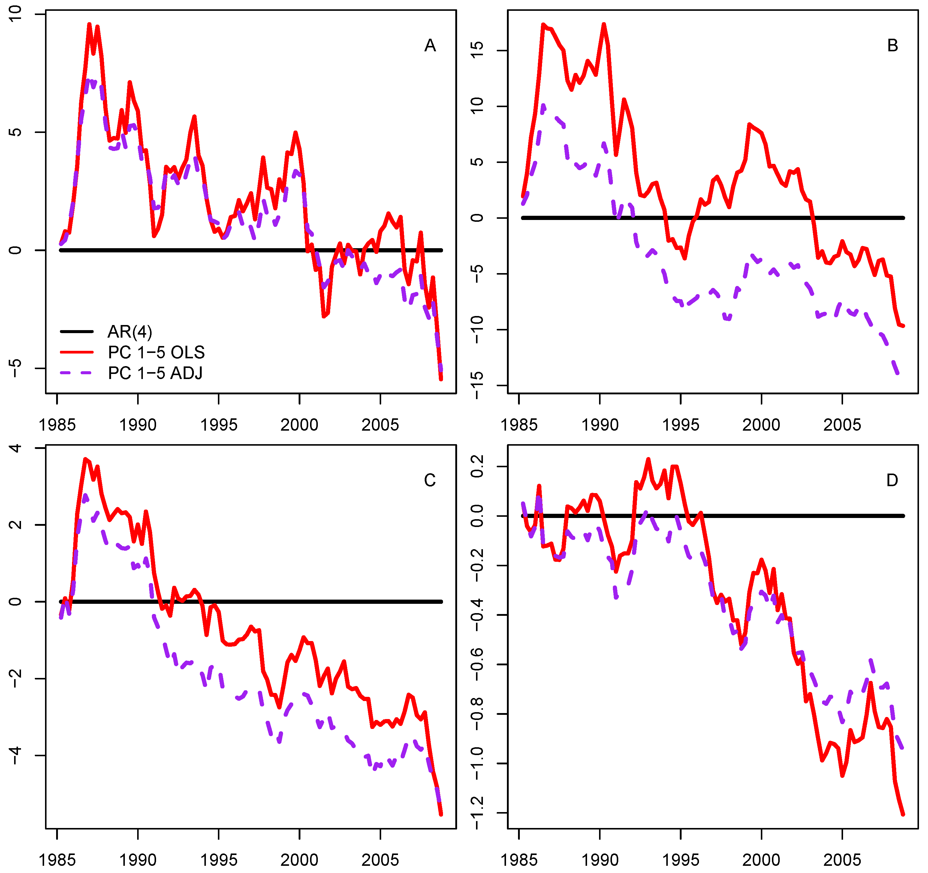
3.2. Forecasting the Major Measures of Economic Activity

In a rolling analysis, each subsample of $n=100$ successive quarters is used to partial out the autoregressive dynamics (up to lag four), estimate the principal components from the residuals, and compute the competing forecasts. Instead of using just a single measure, e.g., the sum of squared prediction errors, for the assessment of the forecasting performance, we prefer to use plots of the cumulative absolute or squared prediction errors, which allows a continuous assessment over the whole evaluation period. However, to save space, we only show the former plots because there are no major discrepancies. An obvious advantage of using absolute errors is that they are less volatile and rankings of the competing forecasts are therefore not so easily inverted by individual extreme errors. Using the autoregression with four lags (AR4) as a benchmark, Figure 1 compares the OLS forecasts based on the first five principal components with the adjusted band regression forecasts obtained from the same principal components by using only the first $r=\left[0.4m\right]$ Fourier frequencies. In one case, the latter forecasts slightly outperform the former, and, in another case, it is the other way round. In two cases, there is practically no difference.

Table 1. Root mean absolute prediction error and root mean squared prediction error by forecasting method and by dependent variable, relative to AR(4) = 1.000; rolling forecasts.

	Ordinary Least Squares		Adjusted-Band-Regression
Group	RMSPE	RMAPE	RMSPE	RMAPE
GDP	0.915	0.965	0.926	0.968
IP	0.971	0.959	0.940	0.939
Employment	0.906	0.919	0.919	0.920
Unemployment	0.884	0.911	0.919	0.930

shows both the root mean absolute prediction error and the root mean squared prediction error relative to the benchmark (value < 1 means better than benchmark) for the two competing forecasts. When we increase the number of principal components from five (used by Stock and Watson 2012) to ten, the adjusted band regression is superior in three of the four case, which shows that the forecasting performance strongly depends on the number of included factors. In the rest of this section, we therefore explore various modifications of the standard factor model, particularly also methods for the automatic selection of the factors to be included in the model. For the assessment of these modifications, only the GDP is used as dependent variable.

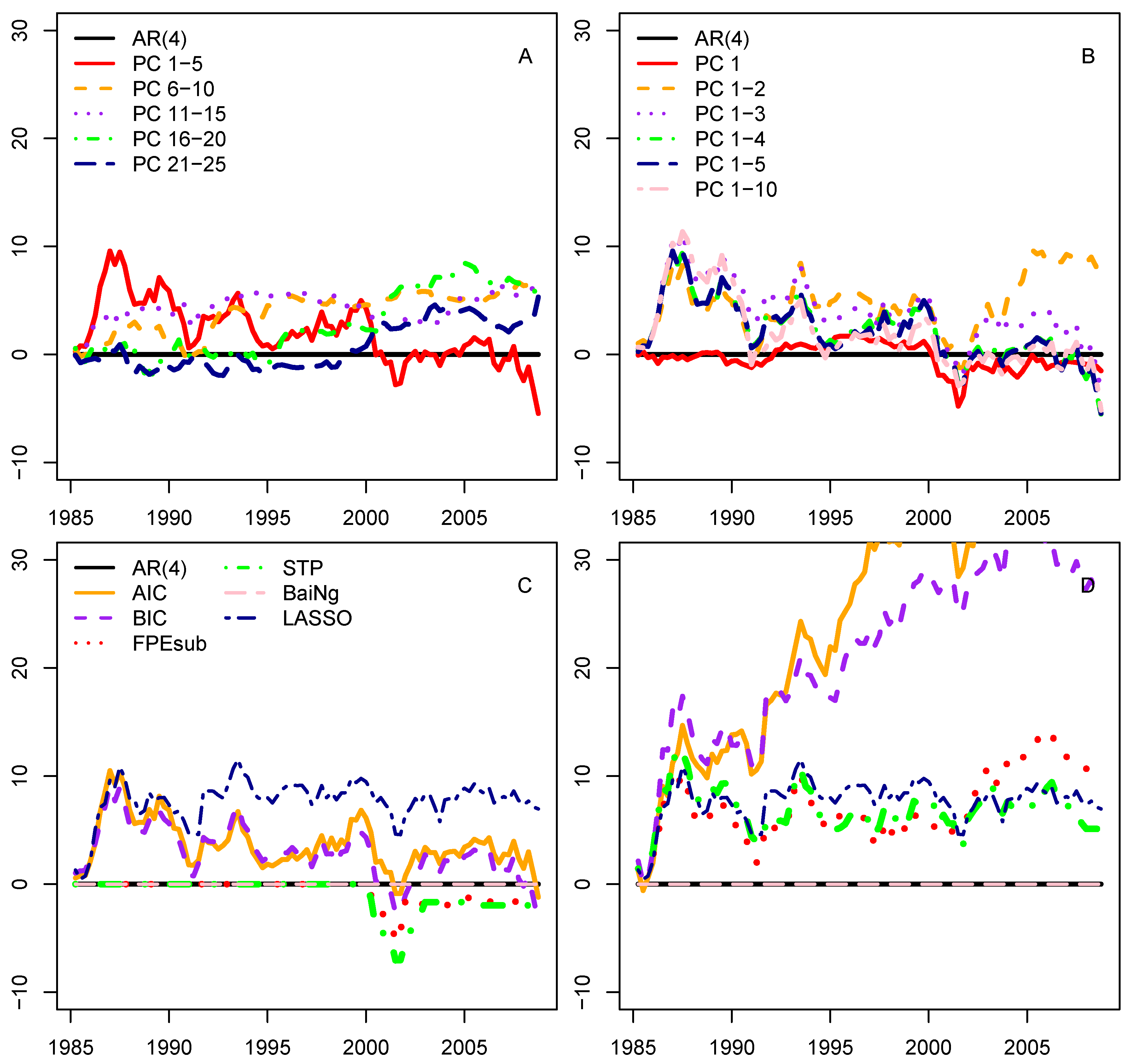
3.3. Selecting the Predictors

Using the GDP as dependent variable, Figure 2A shows the performance of the OLS forecasts when only the first five, the second five, the third five, etc. principal components are included in the model. Apparently, only the forecast using the first five principal components (PCs 1–5) can compete with the benchmark. Figure 2B shows the performance of the OLS forecasts when only the first, the first two, the first three, etc. principal components are included in the model. There is hardly any difference between the models with five and ten principal components, respectively.

Since quarterly macroeconomic series as well as the relationships between them are typically dominated by their low frequency components, we may expect that the first principal components in their effort to explain as much variation as possible focus primarily on the lower frequencies while the other principal components must deal with the rest. The leading principal components might therefore be more informative than the ones following behind. Figure 3 suggests that this is indeed the case. The periodograms of the first and second principal component have a peak close to frequency zero (see Figure 3A,B) while the periodograms of the 89th and 90th principal component are featureless and resemble periodograms obtained from white noise (see Figure 3C,D).

Instead of using a fixed number of principal components, we might try to choose the optimum number with the help of a model selection criterion. AIC and BIC choose the first three or four principal components while ${\mathrm{FPE}}_{\mathrm{sub}}$ and STP select not a single one until around the short recession in 2001. The most parsimonious criterion is the Bai–Ng (denoted as BIC3 on page 201 in Bai and Ng 2002), which copies the benchmark line and selects nothing at all. The other extreme is the prediction by LASSO2 selecting over 10 factors during the entire evaluation period leading to the overall worst performance under the nested setup. As discussed in Section 2.3, when not the h first principal components (ordered according to the size of the eigenvalues) are chosen for a model of dimension h but rather the h best fitting of the $K=90$ first principal components, AIC and BIC are no longer suitable. In the former case (nested models), there is only one model for each h, whereas, in the latter case (nonnested models), there are $K!/(h!(Kh)!)$ models for each h, from which the best fitting model is selected. The orthogonality of the principal components allows us to find the best fitting model for each model dimension h just by running K regressions with only a single principal component and choosing the h best fitting principal components. Despite the computational simplicity of this procedure, the chosen models must still be regarded as the best of a large number of models of the same dimension, hence there is a huge danger of a data-snooping bias, which must be taken care of. Not surprisingly, AIC and BIC fail to do so and therefore always select a much too large model dimension and consequently perform much worse than the other criteria (see Figure 2D). In general, there is obviously no need to change the natural order of the principal components on the basis of their correlations with the dependent variable.

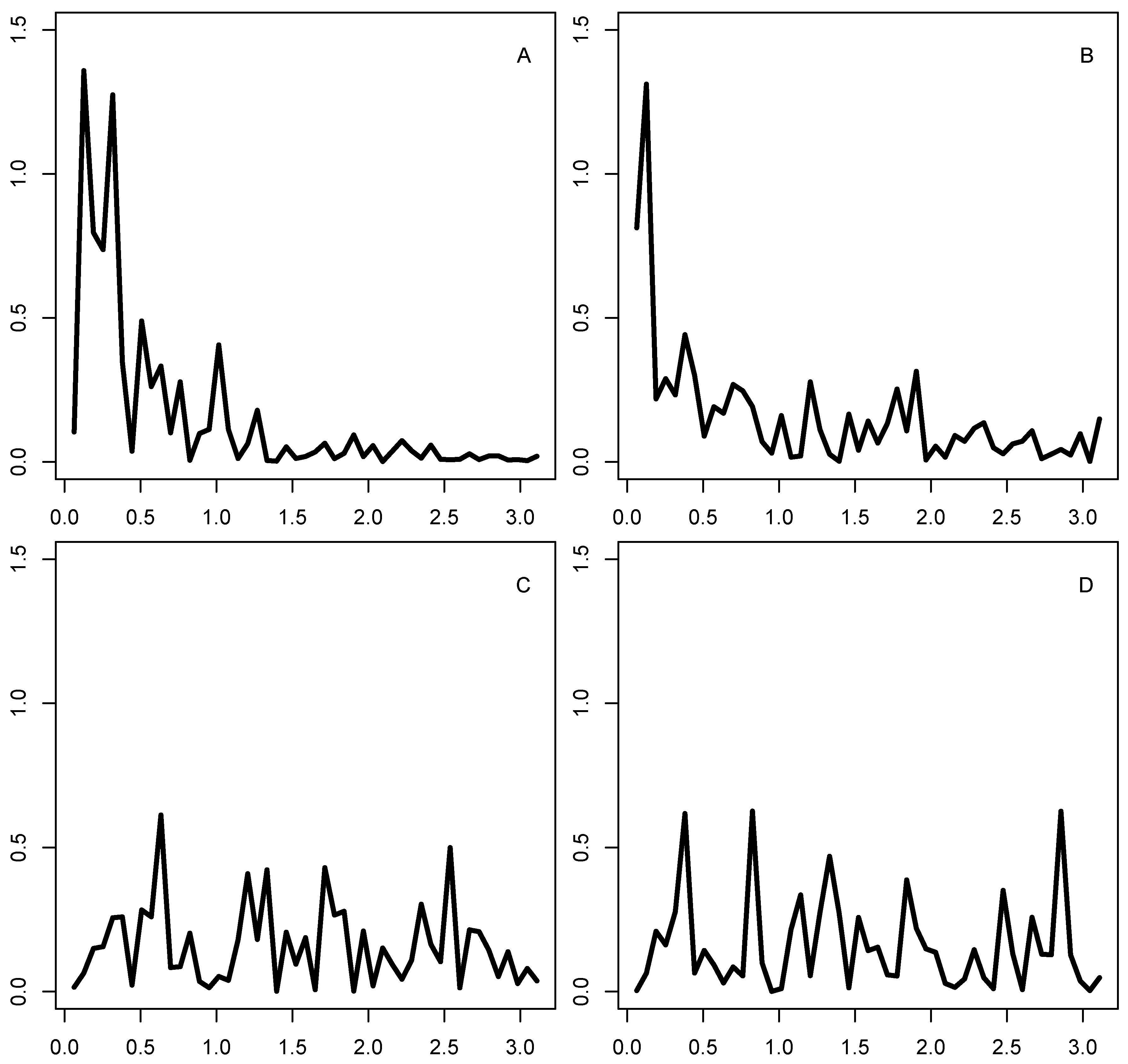
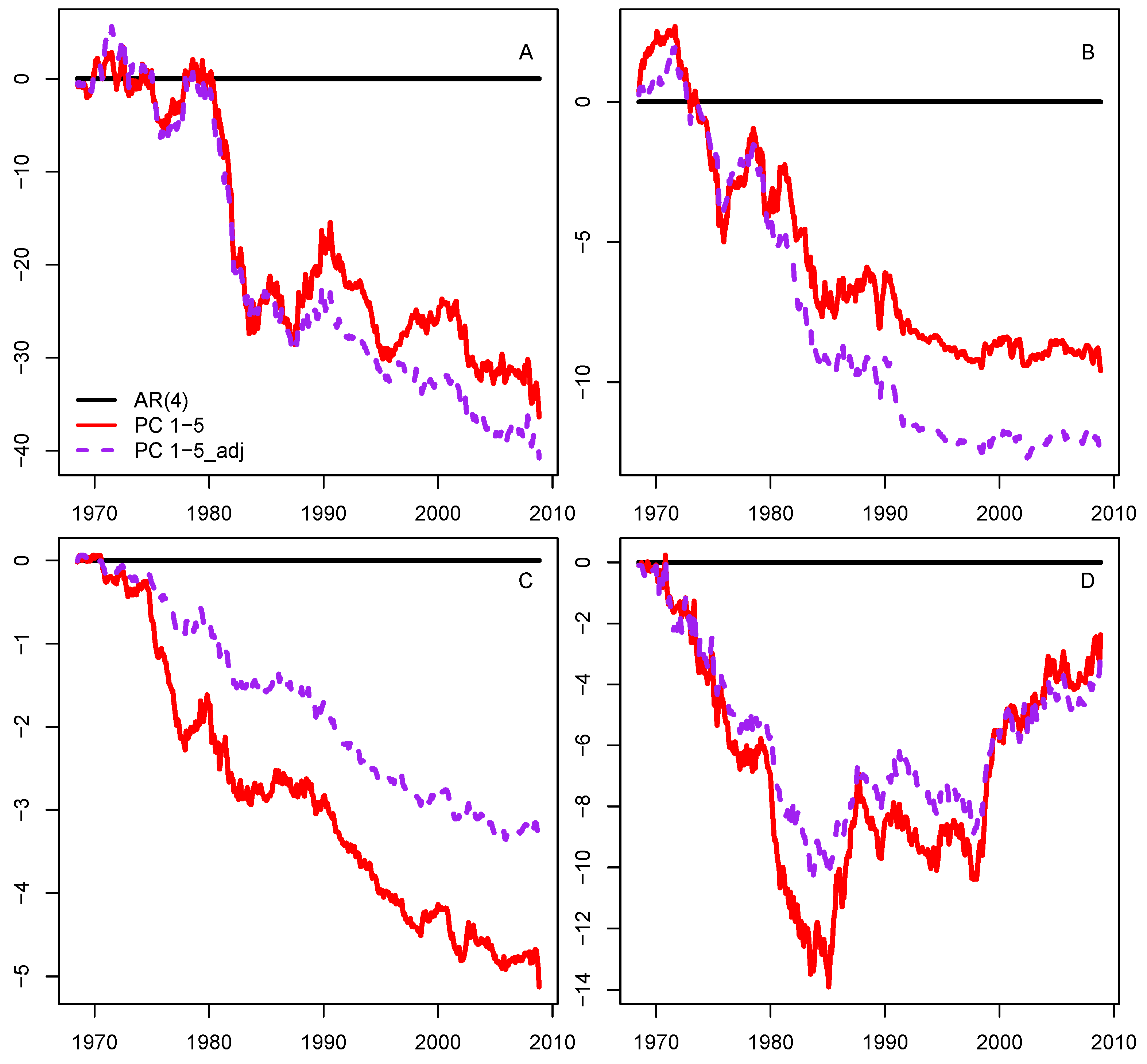
3.4. Using Frequency-Domain Information in Case of Small Subsets of Predictors

In this subsection, we use only small subsets of the original 109 low-level aggregates. We obtain3 these subsets of “targeted predictors” (see Bai and Ng 2008a) with the help of LASSO independently for each subsample in the rolling analysis. Alternatively, the elements of the subsets are fixed as the ten GDP components. Despite the small number of predictors, we still switch to factors/principal components to benefit from their orthogonality properties and further reduce the model dimension without compromising the precision of the forecast. Figure 4 shows that the adjusted band regression forecasts based on the principal components of the second subset (which has been chosen by economic arguments rather than statistical arguments) perform best.

4. Discussion

Using the macroeconomic dataset of Stock and Watson (2012), we explored various methods to improve the performance of the standard factor-augmented forecast, which is based on lagged values of the variable of interest and a small number of factors obtained from a large set of predictors. We found that the use of automatic criteria for the selection of the optimal subset of factors is not helpful, whether the order of the factors is fixed or not. Focusing on the low-frequency components of the factors and disregarding the high-frequency components, which can technically be achieved by dismissing OLS regression in favor of adjusted band-regression, is more promising. However, the results are mixed and depend on the variables to be predicted and on the model specifications. In the case of the gross domestic product, the best results were obtained when the frequency-domain approach was combined with a preselection of a small subset of predictors, which was then used for the calculation of the factors.

From the four major measures of economic activity used in our empirical study, namely gross domestic product, industrial production, employment, and unemployment, the last three are also available as monthly time series. However, the typical spectral shapes of quarterly and monthly time series are very different in nature. While the former are dominated by their low-frequency components, the latter often also have considerable power in the high-frequency band, which makes the use of a band regression approach more difficult. Although the adaption of the forecasting procedure to monthly series is certainly doable, it would possibly be better to leave it for future research. For the time being, we have to be satisfied with Figure 5, which is analogous to Figure 1, but includes M2 money stock instead of GDP and does not yet take into account the differences between quarterly and monthly time series. It compares the performance of the OLS forecasts and the adjusted band regression forecasts. The results are mixed. The adjusted band regression forecasts perform better in two cases and worse in one case. In one case, there is practically no difference.

References

1. Akaike, H. 1969. Fitting autoregressive models for prediction. Annals of the institute of Statistical Mathematics 21: 243–47. [Google Scholar] [CrossRef]
2. Akaike, H. 1998. Information Theory and an Extension of the Maximum Likelihood Principle. New York: Springer, pp. 199–213. [Google Scholar]
3. Altissimo, F., R. Cristadoro, M. Forni, M. Lippi, and G. Veronese. 2010. New eurocoin: Tracking economic growth in real time. The Review of Economics and Statistics 92: 1024–34. [Google Scholar] [CrossRef]
4. Bai, J., and S. Ng. 2002. Determining the number of factors in approximate factor models. Econometrica 70: 191–221. [Google Scholar] [CrossRef] [Green Version]
5. Bai, J., and S. Ng. 2006. Evaluating latent and observed factors in macroeconomics and finance. Journal of Econometrics 131: 507–37. [Google Scholar] [CrossRef]
6. Bai, J., and S. Ng. 2008a. Forecasting economic time series using targeted predictors. Journal of Econometrics 146: 304–17. [Google Scholar] [CrossRef] [Green Version]
7. Bai, J., and S. Ng. 2008b. Large dimensional factor analysis. Foundations and Trends in Econometrics 3: 89–163. [Google Scholar] [CrossRef] [Green Version]
8. Chen, L., J. J. Dolado, and J. Gonzalo. 2014. Detecting big structural breaks in large factor models. Journal of Econometrics 180: 30–48. [Google Scholar] [CrossRef] [Green Version]
9. Cheng, X., and B. Hansen. 2015. Forecasting with factor-augmented regression: A frequentist model averaging approach. Journal of Econometrics 186: 280–93. [Google Scholar] [CrossRef] [Green Version]
10. Connor, G., and R. A. Korajczyk. 1993. A test for the number of factors in an approximate factor model. The Journal of Finance 48: 1263–91. [Google Scholar] [CrossRef]
11. Eickmeier, S., and C. Ziegler. 2008. How successful are dynamic factor models at forecasting output and inflation? A meta-analytic approach. Journal of Forecasting 27: 237–65. [Google Scholar] [CrossRef]
12. Engle, R. F. 1974. Band spectrum regression. International Economic Review 15: 1–11. [Google Scholar] [CrossRef]
13. Forni, M., M. Hallin, M. Lippi, and L. Reichlin. 2000. The generalized dynamic-factor model: Identification and estimation. The Review of Economics and Statistics 82: 540–54. [Google Scholar] [CrossRef]
14. Foster, D., and E. George. 1994. The risk inflation criterion for multiple regression. Annals of Statistics 22: 1947–75. [Google Scholar] [CrossRef]
15. George, E., and D. Foster. 2000. Calibration and empirical bayes variable selection. Biometrika 87: 731–47. [Google Scholar] [CrossRef] [Green Version]
16. Hannan, E. 1963. Regression for time series. In Proceedings of the Symposium on Time Series Analysis. Edited by M. Rosenblatt. New York: John Wiley and Sons Inc., pp. 14–37. [Google Scholar]
17. Johnson, N. L., D. Rothman, R. G. Krutchkoff, P. A. Lachenbruch, and R. R. Hocking. 1968. Letters to the editor. Technometrics 10: 423. [Google Scholar]
18. Kim, H. H., and N. R. Swanson. 2014. Forecasting financial and macroeconomic variables using data reduction methods: New empirical evidence. Journal of Econometrics 178: 352–67. [Google Scholar] [CrossRef] [Green Version]
19. Müller, U., and M. Watson. 2016. Measuring uncertainty about long-run predictions. Review of Economic Studies 83: 1711–40. [Google Scholar] [CrossRef] [Green Version]
20. Phillips, P. B. C. 1991. Spectral regression for co-integrated time series. In Nonparametric and Semiparametric Methods in Economics and Statistics. Edited by W. Barnett, J. Powell and G. Tauchen. Cambridge: Cambridge University Press. [Google Scholar]
21. Reschenhofer, E. 2004. On subset selection and beyond. Advances and Applications of Statistics 4: 265–86. [Google Scholar]
22. Reschenhofer, E. 2010. Discriminating between non-nested models. Far East Journal of Theoretical Statistics 31: 117–33. [Google Scholar]
23. Reschenhofer, E. 2015. Consistent variable selection in large regression models. Journal of Statistics: Advances in Theory and Applications 14: 49–67. [Google Scholar]
24. Reschenhofer, E., and M. Chudy. 2015a. Adjusting band-regression estimators for prediction: Shrinkage and downweighting. International Journal of Econometrics and Financial Management 3: 121–30. [Google Scholar]
25. Reschenhofer, E., and M. Chudy. 2015b. Imposing frequency-domain restrictions on time-domain forecasts. Journal of Statistical and Econometric Methods 4: 1–16. [Google Scholar]
26. Reschenhofer, E., D. Preinerstorfer, and L. Steinberger. 2013. Non-monotonic penalizing for the number of structural breaks. Computational Statistics 28: 2585–98. [Google Scholar] [CrossRef]
27. Reschenhofer, E., M. Schilde, E. Oberecker, E. Payr, H. Tandogan, and L. Wakolbinger. 2012. Identifying the determinants of foreign direct investment: A data-specific model selection approach. Statistical Papers 53: 739–52. [Google Scholar] [CrossRef]
28. Schwarz, G. 1978. Estimating the dimension of a model. The Annals of Statistics 6: 461–64. [Google Scholar] [CrossRef]
29. Stock, J., and M. W. Watson. 2009. Forecasting in Dynamic Factor Models Subject to Structural Instability. Oxford: Oxford University Press, pp. 1–57. [Google Scholar]
30. Stock, J., and M. Watson. 2012. Generalised shrinkage methods for forecasting using many predictors. Journal of Business and Economic Statistics 30: 482–93. [Google Scholar] [CrossRef]
31. Stock, J., and Mark W. Watson. 2002. Forecasting using principal components from a large number of predictors. Journal of the American Statistical Association 97: 1167–79. [Google Scholar] [CrossRef] [Green Version]
32. Tibshirani, R. 1996. Regression shrinkage and selection via the lasso. Journal of the Royal Statistical Society. Series B (Methodological) 58: 267–88. [Google Scholar] [CrossRef]
33. Tibshirani, R., and K. Knight. 1999. The covariance inflation criterion for adaptive model selection. Journal of the Royal Statistical Society: Series B (Statistical Methodology) 61: 529–46. [Google Scholar] [CrossRef]
1.
2.
The tuning parameter λ , which controls for the parsimonity of the LASSO procedure, is selected by leave-one-out cross validation at each rolling iteration.
3.
Note that in Section 3.3, we use LASSO for selecting the factors, whereas here we use LASSO for preselecting the predictors.
Figure 1. Cumulative sums of absolute prediction errors relative to AR4 benchmark (black) for OLS forecasts based on first five principal components (red) and adjusted band regression forecasts based also on the first five principal components (violet). The (quarterly) dependent variables to be forecasted are: (A) gross domestic product; (B) industrial production; (C) employment; and (D) unemployment.
Econometrics 07 00046 g001
Figure 2. Cumulative sums of absolute prediction errors relative to AR4 benchmark (black) for OLS forecasts based on: (A) first five, second five, third five, etc. principal components obtained from all predictors; (B) first, first two, first three, etc. principal components obtained from all predictors; and (C) first h principal components, where h is chosen by AIC, BIC, FPE sub , STP, BaiNg and LASSO, (D) h best fitting principal components, where h is chosen by AIC, BIC, LASSO, etc.
Econometrics 07 00046 g002
Figure 3. Periodograms of the kth principal component for: (A) k = 1 ; (B) k = 2 ; (C) k = 89 ; and (D) k = 90 .
Econometrics 07 00046 g003
Figure 4. Cumulative sums of absolute prediction errors relative to AR4 benchmark (black) for OLS forecasts (A,C) and adjusted band regression (B,D) based on the first, the first two, the first three, and principal components obtained from a subset of all predictors preselected by LASSO (A,B) and the subset containing only the ten GDP components (C,D), respectively.
Econometrics 07 00046 g004
Figure 5. Cumulative sums of absolute prediction errors relative to AR4 benchmark (black) for OLS forecasts based on first five principal components (red) and adjusted band regression forecasts based also on the first five principal components (violet). The (monthly) dependent variables to be forecasted are: (A) industrial production; (B) employment; (C) unemployment; and (D) M2 money stock.
Econometrics 07 00046 g005