1. Introduction
Nonparametric regression is an important tool for exploring the unknown relationship between a response variable and a set of explanatory variables also known as regressors. A simple and commonly used estimator of the regression function is the Nadaraya-Watson (NW) estimator proposed by [
1,
2]. In many empirical applications of nonparametric regression models, regressors are often of mixed types such as continuous and categorical. In such a situation, [
3] proposed estimating the regression function by the NW-type estimator with different types of regressors being assigned different kernel functions. Since their seminal work, there have been many theoretical and methodological investigations on nonparametric regression with mixed types of regressors (see for example, [
4,
5,
6,
7,
8,
9,
10,
11]). It has been generally accepted that the performance of the NW estimator is mainly determined by its bandwidths. In the current literature, the cross-validation (CV) technique is often used for choosing bandwidths. Following the recent work by [
12], this paper aims to investigate a Bayesian sampling approach to bandwidth estimation for the NW estimator in a nonparametric regression model, where regressors can be continuous and discrete variables.
The popularity of CV is accredited to its simplicity and reasonably good performance. However, this bandwidth selection method has some limitations. First, the CV technique tends to choose a too small bandwidth. As discussed by [
13], there are necessary and sufficient conditions to ensure the optimality of CV for bandwidth selection in nonparametric regression models. It may not be possible to examine whether these conditions hold in practice. Second, even though the CV method does not require an assumption about the error density, it provides no direct solutions to error density estimation. However, error density estimation is important for assessing the goodness of fit of a specified error distribution [
14,
15,
16]; for testing symmetry, skewness and kurtosis of the residual distribution [
17,
18,
19]; for statistical inference, prediction and model validation [
20,
21]; and for estimating the density of the response variable [
22,
23]. Therefore, being able to estimate the error density is as important as being able to estimate the regression function.
We present a Bayesian sampling approach to bandwidth estimation for the NW estimator involving mixed types of regressors, where the errors are independent identically distributed (iid) and follow a kernel-form error density studied previously by [
24] for GARCH models, and [
12] for nonparametric regression models with only continuous regressors. We develop a sampling algorithm, which is an extension to the algorithm proposed by [
12] in the sense that the regressors are of mixed types. It leads to a posterior estimate of the response density, where the response variable is modeled as an unknown function of continuous and discrete explanatory variables. The importance of such models can be explained through finance and economic data examples.
1Suppose we are interested in the distribution of daily returns of the All Ordinaries (Aord) index of the Australian stock market. Many analysts believe that since the beginning of the global financial crisis, the Australian stock market generally follows the overnight performance of the US and several European markets. As the US stock market is thought to have a leading effect on other markets worldwide, we may choose the daily return of the S&P 500 index as a regressor, and a binary variable indicating the sign of the daily return of FTSE index as another regressor. With our proposed sampling algorithm, we are able to not only estimate bandwidths for the NW estimator and the kernel-form error density, but also derive a posterior estimate of the response density. When CV is used to choose bandwidths for the NW estimator, one might have to apply likelihood cross-validation to the residuals so as to derive a kernel density estimator of residuals. This would result in a two-stage procedure for choosing bandwidths in the regression and error-density estimators, and we show that it is empirically inferior to our sampling procedure through a series of simulation studies.
We conduct Monte Carlo simulation studies to compare the in-sample and out-of-sample performances between Bayesian sampling and CV in choosing bandwidths for the regression estimator and error density estimator. Our Bayesian sampling approach to bandwidth estimation leads to more accurate estimators than CV in most situations and in particular for smaller sample sizes, while the latter performs as well as the former in only a few occasions.
Our sampling algorithm is empirically validated through an application to bandwidth estimation in the nonparametric regression of the Aord daily return on the overnight S&P 500 return and a binary variable showing the sign of overnight FTSE return. An important and very useful output from this sampling algorithm is the one-day-ahead posterior predictive density of the Aord daily return, which we use to calculate value-at-risk (VaR). Given the close relationship between conditional mean regression and conditional density estimation, we also modify the sampling algorithm for the purpose of choosing bandwidths in kernel condition density estimation of GDP growth rate of a country given its OECD status and the year value of growth-rate observations.
The rest of the paper is organized as follows.
Section 2 presents a brief description of the NW estimator when the regressors include continuous and discrete variables. In
Section 3, we derive the likelihood and posterior for bandwidth parameters. A sampling algorithm is also presented.
Section 4 presents Monte Carlo simulation studies that examine the performance of the proposed sampling method for bandwidth estimation. In
Section 5, we use the sampling method to estimate bandwidths for a nonparametric regression model of stock returns. We modify the proposed sampling algorithm to estimate bandwidths in kernel conditional density estimation of a country’s GDP growth rate in
Section 6.
Section 7 concludes the paper.
2. Nadaraya-Watson Estimator with Mixed Types of Regressors
We present a brief description of the NW estimator of the unknown regression function that contains continuous and discrete explanatory variables. More details can be found in [
6]. We consider the nonparametric regression model given by
where
is an observation of a scalar response,
with
being a vector of
p continuous variables and
a vector of
q discrete variables, and
are iid errors with an unknown probability density function denoted as
. The discrete variables can be either ordered or unordered, which in turn affects the choice of kernel functions.
The flexibility of model (1) stems from the fact that the unknown regression function
does not need to have a specific functional form. With some smoothness properties,
is estimated by the NW estimator of the form given by
where
is a generalized product kernel that admits continuous and discrete regressors. There is a wide range of kernel functions for continuous type of variables (see for example, [
6]), and kernel functions for discrete type of variables (see for example, [
27]). Here, the kernel function for continuous regressors is a product of
p identical Gaussian kernel functions expressed as
where
and
are respectively, the
jth elements of
and
,
is a vector of bandwidths associated with the
p continuous regressors, and
is the standard Gaussian density being used as the kernel function for a continuous variable throughout this paper.
The kernel function for discrete regressors is a product of
q identical discrete kernel functions expressed as
If the
jth element of
is nominal, the kernel function is Aitchison and Aitken’s kernel [
28] given by
where
and
are respectively, the
jth elements of
and
, and
is the bandwidth, for
, and
denotes the number of discrete outcomes. Note that this kernel function can be used for either unordered categorical variables or unequal-interval ordered variables.
If the
jth element of
is ordinal, its kernel is Li and Racine’s kernel [
6] kernel expressed as
for
, and
, where
is a vector of bandwidths assigned to the corresponding
q discrete regressors. These bandwidths are restricted to be within
.
For the case where discrete explanatory variables are included in a nonparametric regression model, there exists a conventional frequency estimator of the regression function in the literature. This frequency approach involves splitting data into cells based on different values of the discrete variables and using the data in each cell to derive an estimator of the regression function. Li and Racine [
6] found that the NW estimator given by (2) is strongly supported against the frequency estimator for both theoretical and practical reasons.
It is noteworthy that if
for all
, then
becomes an indicator function taking values 1 and 0, corresponding to the conventional frequency estimator. When
, this indicates that
is “smoothed out” and becomes an irrelevant variable [
5]. Similarly, if
is very large in the kernel function given by (2), it indicates that
is smoothed out and has no explanatory effect on the response variable. As a by-product, the ability of distinguishing irrelevant variables from relevant variables makes the resulting NW estimator very attractive, in comparison to the conventional frequency estimator.
The performance of the NW estimator is mainly determined by its bandwidths, and in the current literature, bandwidths are often chosen through CV with the CV function defined as
where
is the leave-one-out NW estimator given by
and
is a weight function taking values in
. The purpose of the weight function in
is to avoid difficulties caused either by division by zero or by the slow convergence rate when
is near the boundary of the support of
x (see [
13]). We follow [
10] and choose
where
is an indicator function, and
and
are the sample mean and standard deviation of
.
In some empirical studies, CV tends to choose too small a bandwidth. Li and Zhou [
13] observed that there are some conditions to ensure the optimality of the CV function. However, it is impossible to check whether all these conditions hold due to the unknown regression function. This problem has motivated us to investigate an alternative approach to bandwidth estimation, namely a Bayesian sampling approach.
3. Bayesian Estimation of Bandwidths
We consider the nonparametric regression model given by (1) and assume that the iid errors follow an unknown distribution with its density approximated by
where
is the standard Gaussian probability density function. Being previously introduced by [
24] in GARCH models, this density function of errors is a mixture of
n identical standard Gaussian densities with different means located at individual errors and a common standard deviation
b. Moreover, from the view of kernel smoothing, this error density can be regarded as a kernel density based on independent errors, where
b plays the role of bandwidth or smoothing parameter. Note that the error density given by (6) is different from the one proposed by [
29], who used residuals as proxies of errors and employed the kernel density estimator of residuals to approximate the true error density.
In order to conduct Bayesian sampling for the purpose of estimating bandwidths, we treat the bandwidths in the NW estimator of the regression function and the kernel-form error density as parameters. Even though chosen bandwidths depend on sample size as revealed by existing asymptotic results, such a treatment will not cause problems for a fixed-size sample (see also [
30,
31,
32]).
Let
, for
, denote the observations of
. Under the error density given by (6), we have
for
. As
is unknown, we replace it with its leave-one-out NW estimator. Thus, the density of
is approximated by
for
.
3.1. An Approximate Likelihood
The vector of all bandwidths denoted as
are treated as parameters, given which we wish to derive an approximate likelihood of
. For this purpose, we cannot use the approximate density of
given by (7) directly because it contains
for
. When
b is a parameter and is estimated based on a fixed-size sample, numerical optimization of the likelihood built up through (7) may end up with an arbitrarily small bandwidth due to the existence of
. Therefore, any pair of observations that leads to a zero argument of
should be excluded from the summation given by (7). Following the suggestion of [
12], we exclude the
jth term when
, from the summation given in (7). Let
and
is the number of terms excluded from the sum given in (7). Although the response variable is continuous, by chance, the set
may contain more than one element. Therefore, the density of
is approximated by
for
.
Let
denote a row vector whose elements are the squared elements of
h. Thus, given
, the likelihood of
y is approximated by
Note that if
, this likelihood function reduces to the leave-one-out likelihood.
3.2. Priors
We follow [
12] choices of priors of bandwidths for continuous regressors and the kernel-form error density. Let
denote the prior of
, for
, and
the prior of
. The priors of
and
can be chosen from a variety of densities with a positive domain, such as log normal and inverse Gamma densities. As the Gaussian kernel is used for each variate in this situation, each bandwidth is also considered as the standard deviation of the corresponding Gaussian density. Therefore, the prior of each squared bandwidth can be chosen to be an inverse Gamma density, which is a frequently used proper prior for the variance parameter. Thus, the prior of
is
and the prior of
is
where the hyperparameters are chosen as
and
(see for example, [
33] and [
34] pp. 38–39).
Let
denote the prior of
, the bandwidth assigned to the
jth discrete regressor, for
. The prior of
is assumed to be a uniform density defined on
. For nominal regressors,
and
; and for ordered categorical regressors,
and
. See for example, [
8], for discussion of restrictions on these smoothing parameters.
The joint prior of is the product of all the marginal priors and is denoted as .
3.3. An Approximate Posterior
An approximate posterior of
is obtained as the product of the approximate likelihood given by (8) and the joint prior, and is expressed as (up to a normalizing constant)
The random-walk Metropolis algorithm can be used to carry out the simulation, where the acceptance rate of random-walk Metropolis algorithm is targeted at 0.234 for multivariate draws and 0.44 for univariate draws [
35,
36]. In order to achieve similar levels of acceptance rates, we use the adaptive random-walk Metropolis algorithm proposed by [
36]. This algorithm is capable of selecting appropriate scales, and achieves the targeted acceptance rates without manual adjustment. The sampling procedure is described as follows.
- Step 1:
Specify a Gaussian proposal distribution, and start the sampling iteration process by choosing an arbitrary value of and denoting it as . For example, the elements of and can be any values on and the elements of can be any values on for nominal regressors and for categorical regressors.
- Step 2:
At the
kth iteration, the current state
is updated as
, where
u is drawn from the proposal density which is the
p dimensional standard Gaussian density, and
is an adaptive tuning parameter with an arbitrary initial value
. The updated
is accepted with a probability given by
- Step 3:
The tuning parameter for the next iteration is set to
where
is a constant, and
ξ is the optimal target acceptance probability, which is 0.234 for multivariate updating and 0.44 for univariate updating (see for example, [
35,
36]).
- Step 4:
Update and in the same way as described by Steps 2 and 3.
- Step 5:
Repeat Steps 2–4, discard the burn-in period of iterations, and the draws after the burn-in period are recorded and denoted as .
Upon completing the above iterations, we use the ergodic mean (or posterior mean) of each simulated chain as an estimate of each bandwidth. The mixing performance of each simulated chain is monitored by the simulation inefficiency factor (SIF). As each simulated chain is a Markov chain, its SIF can be interpreted as the number of draws required so as to derive independent draws from the simulated chain (see for example, [
33,
37,
38,
39]).
In the following analyses, the burn-in period is taken as 1000 iterations and the number of recorded iterations after the burn-in period is . The number of batches is 200, and there are 50 draws within each batch.
4. Monte Carlo Simulation Study
A Monte Carlo simulation study was conducted to investigate the properties of the proposed Bayesian sampling approach to bandwidth estimation in comparison to the CV method for bandwidth selection in the NW regression estimator. The conventional frequency estimator, which is equivalent to setting the bandwidths for all discrete and continuous regressors to zero in the NW estimator [
6] (Chapter 3) was also included in the comparison.
A range of different simulation experiments were conducted using seven different data generating processes (DGPs), five of which were discussed in [
4]. To assess the performance of each approach, at each iteration we generated
observations denoted as
, where
is calculated via the DGP,
is the vector of discrete regressors and
is the vector of continuous regressors. The first
n observations were used for estimation and in-sample evaluation, and the last
n observations for out-of-sample evaluation (see also [
10]). We used the average squared error (ASE) as an evaluation measure for both in-sample and out-of-sample evaluation:
where
under the Bayesian method,
under CV, and
for the frequency estimator;
is the NW estimator of
m based on the sample of the first
n observations, and
is the weight function given by (5) for the in-sample and out-of-sample evaluation. The purpose of the weight function is to trim those extreme observations that lie outside most of the data points in the continuous regressors [
4]. We calculated the mean, median, standard deviation (SD) and interquartile range (IQR) of each ASE averaged over the 1000 Monte Carlo replications.
In order to test whether variations in in-sample ASE between the different estimation methods are significantly different, we conducted the Kruskal-Wallis test [
40]. When the Kruskal-Wallis test rejects the null hypothesis of no difference among the methods considered, we implement a posthoc multiple comparison, which is Dunn’s test [
41] with Bonferroni correction, to examine which method differs significantly from others. Differences in out-of-sample ASEs were assessed using the model confidence set (MCS) procedure of [
42].
4.1. Accuracy of Regression Estimator
4.1.1. Experiment 1: Binary and Continuous Regressors
This experiment involves three DGPs. The first DGP is given by
for
, where
takes values of 0 and 1 with an equal probability of 0.5,
,
is drawn from the uniform distribution on
,
;
, and
is drawn from
. Sample sizes of
, 200 and 500 were used, and the results are presented in
Table 1.
The NW estimator with bandwidths estimated through Bayesian sampling slightly outperforms the same estimator with bandwidths selected through CV, and these methods outperform the conventional frequency estimator in terms of all four summary statistics. The differences decline as n increases. The Kruskal-Wallis test has a p value of zero for each value of n implying that there are significant differences in performance between at least one pair of methods. According to Dunn’s test with Bonferroni correction, the Bayesian method differs significantly from the frequency method for all sample sizes, but differs significantly from the CV method for only. For and 500, differences between the Bayesian and CV methods are insignificant. Based on the out-of-sample ASE values, the MCS procedure determines that the Bayesian method performs best for all values of n.
The second and third DGPs are given by
and
for
, where
and
take values from
with equal probabilities of 0.5,
and
are drawn from
, and
is drawn from
. The third DGP differs from the second by the inclusion of two interaction terms. Again, sample sizes of
, 250 and 500 were used. The results are presented in
Table 2.
To estimate the regression functions for the two DGPs, we employed the NW estimator with bandwidths estimated through Bayesian sampling and CV, as well as the conventional frequency estimator. The summary statistics for the in-sample and out-of-sample ASE values for both DGPs are tabulated in
Table 2.
For the second DGP, Bayesian sampling leads to a slightly better NW estimator than CV in most cases based on the summary statistics of ASE values, but these differences are not significant because the Kruskal-Wallis test cannot reject the null hypothesis of no differences between the three methods for all three sample sizes. Using the out-of-sample ASE values, the MCS procedure finds in favour of the Bayesian approach for and the CV method for and 500.
For the third DGP, the Kruskal-Wallis test clearly rejects the null hypothesis of no difference between the three methods for all values of n. Using Dunn’s test with Bonferroni correction, we found that the Bayesian method differs significantly from the CV and frequency methods respectively. However, the CV method does not differ significantly from the frequency method. The MCS procedure finds that under the out-of-sample ASE, the Bayesian method performs better than the CV method, and both methods outperform the frequency approach.
4.1.2. Experiment 2: Ordered and Unordered Categorical Regressors
The fourth and fifth DGPs were used to examine the difference between kernel functions for ordered categorical variables given by (4) and those for unordered categorical variables given by (3). The fourth DGP includes ordered categorical and continuous variables and is expressed by
where
is drawn from
, for
and 2,
takes values from
with an equal probability of
, for
and 2, and the error term
is drawn from
, for
.
Let
denote the vector of two continuous regressors and
the vector of two discrete regressors. The relationship between the response and regressors is modeled by
where
, for
, are assumed to be independent. Bandwidths in the NW regression estimator are estimated through the proposed Bayesian method and the CV approach each applied in two different ways; first using the kernel for ordered categorical variables given by (4) and then using the kernel for unordered categorical variables given by (3). Together with the conventional frequency estimator, this means that we are now evaluating five different estimators. We expect that the use of the ordered kernel should dominate the use of the unordered kernel because the observations of the discrete regressors have a natural order. Sample sizes of
, 200, 500 and 1000 were used and the results are presented in
Table 3.
The Kruskal-Wallis test has a p value of zero for all values of n thus rejecting the null hypothesis of no difference in performance among the five estimators. According to the in-sample and out-of-sample ASE measures, the Bayesian method performs slightly better than the corresponding CV method, and the use of the kernel function for the ordered variables outperforms the use of the kernel function for the unordered variables. The Bayesian method using the ordered kernel almost always has the lowest values of all four summary statistics for both in-sample and out-of-sample ASEs. Applying Dunn’s test with Bonferroni correction to the in-sample ASEs, we found that the Bayesian method with ordered kernel is similar to the Bayesian method with unordered kernel and CV with ordered kernel, but differs from the CV method with unordered kernel and frequency method for all sample sizes. The Bayesian method with unordered kernel differs from the CV method with ordered and unordered kernels and frequency method when . As n increases, the Bayesian method differs only from the CV with unordered kernel and frequency method. There are significant differences between the CV method with ordered and unordered kernels and frequency method. The MCS procedure finds that the ordered kernel should be used for ordered categorical variables, and the Bayesian method performs better than the CV method.
The fifth DGP includes ordered categorical and continuous regressors and is given by
where
is drawn from
with an equal probability of 1/5,
is drawn from
, and the error term
is drawn from
. As the response variable is affected by the discrete regressor through its square root, the actual distance between categories 0 and 1 is 1, between categories 1 and 2 is
, between categories 2 and 3 is
, and between categories 3 and 4 is
(see also [
4]).
The purpose of this simulation is to investigate the five estimators in a situation where the distance between any pair of successive observations is not a fixed constant. Sample sizes of
, 100 and 200 were used, and the results are presented in
Table 4.
Again the Kruskal-Wallis test has a p value of zero for all values of n thus rejecting the null hypothesis of no difference in performance among the five estimators. This time the Bayesian method using the unordered kernel almost always has the lowest values of all four summary statistics for both in-sample and out-of-sample ASEs. Differences diminish as n increases. According to Dunn’s test with Bonferroni criterion, the Bayesian method with ordered and unordered kernels behave similarly, while the CV method with unordered kernel performs similarly to the frequency method. There are significant differences among the Bayesian method with unordered kernel, CV with ordered and unordered kernels, and frequency methods. Based on the in-sample ASEs, the ordered Bayesian method is also better than both CV methods and the frequency approach for all values of n. Not surprisingly, the MCS procedure finds in favour of the Bayesian method using the unordered kernel for all n values.
What is surprising is that differences between the CV method with unordered kernel and the frequency approach are not significant. In order to examine the role of the choice of kernel in the relative performance of the various estimators, we repeated the last simulation using Wang and Van Ryzin’s kernel function [
43], where bandwidths were estimated through Bayesian, CV and frequency approaches.
Table 5 presents a summary of descriptive statistics of the in-sample and out-of-sample ASE values. Under the criterion of in-sample ASE, the frequency approach is comparable to the Bayesian method, but both perform poorer than CV. However, under the criterion of out-of-sample ASE, the Bayesian approach is comparable to CV, but both perform better than the frequency approach. The Kruskal-Wallis test reveals no significant differences between the three methods for all values of
n.
4.1.3. Experiment 3: Time Series Regression with Continuous and Binary Regressors
The sixth DGP includes a time series response variable explained by its lagged variable, a continuous time series regressor
and a binary regressor
, which is generated based on another time series. This model is expressed as
for
, where
r is a random number that follows the uniform distribution on
, and
are iid
. The continuous regressor
is generated as
where
are iid
. The binary regressor
is an indicator of
and equals one with a positive
and zero otherwise, where
is generated as
where
are iid
. The variance-covariance matrix of
, for
, is
Sample sizes of
, 200 and 500 were used in this experiment and the results are presented in
Table 6.
The Kruskal-Wallis test rejects the null hypothesis of no difference between the ASEs of the three methods for but not for and 500. The Bayesian method always has the smallest mean ASE and almost always has the smallest median across both in-sample and out-of-sample ASEs. According to Dunn’s test with Bonferroni correction, the Bayesian method significantly differs from the frequency method, while the CV method performs similarly to the Bayesian and frequency methods for . For this sample size, the in-sample and out-of-sample mean ASEs obtained through CV are respectively, 8.8% and 23.2% larger than those for the Bayesian method. Based on the MCS procedure applied to the out-of-sample ASEs, the Bayesian method is significantly better than its two counterparts.
4.1.4. Experiment 4: The Presence of Irrelevant Regressors
In a nonparametric regression model, the NW estimator has the ability to smooth out irrelevant regressors through a data-driven bandwidth selection method such as CV by choosing very large bandwidth parameters for those regressors. This has important implications for variable selection (see [
5]). This experiment compares the Bayesian and CV methods in the presence of two irrelevant regressors.
The seventh DGP generates variables as follows. Binary variables
and
were generated so that
and
and continuous variables
and
were generated as independent standard normal values for
. They were generated so there is no correlation between any pair of regressors. The response variable was generated via
where
, for
. In order to examine whether irrelevant regressors can be smoothed out by assigning them large bandwidths, we estimate the following model:
for
. This model means that
and
are irrelevant regressors. Samples sizes of
and 250 were used. Summary statistics of the estimated bandwidths for 1000 iterations are presented in
Table 7 with the summary statistics for the ASEs of the two methods given in
Table 8.
For the proposed Bayesian bandwidth selection method, the average bandwidth chosen for is larger than that chosen for by 1.47 times when (3.87 times when ), and the average bandwidth chosen for is larger than that chosen for by 3.92 times when (3.87 times when ). This shows that due to their large bandwidths, irrelevant regressors may not explain too much about the response variable in comparison to their corresponding relevant regressors.
When CV is used for bandwidth choice, we find that the average bandwidth chosen for is larger than the one chosen for by 5.23 times when (12.13 times when ). Moreover, the average bandwidth chosen for is larger than that chosen for by times when ( times when ). Clearly, CV leads to a larger bandwidth than the Bayesian approach for each irrelevant regressor.
With respect to the ASE measure of accuracy, the proposed Bayesian sampling method leads to slightly better accuracy than CV when with CV being better when . The Kruskal-Wallis test rejects the null hypothesis at the 5% significance level of no difference between the two methods for both sample sizes. Having implemented Dunn’s test with Bonferroni criterion, we found that the Bayesian method differs significantly from the CV method for all sample sizes. The MCS procedure applied to the out-of-sample ASEs finds the Bayesian method is significantly better when and CV is significantly better when .
In the above seven simulation studies, we only consider certain types of discrete variables such as binary and categorical variables. We have not considered DGPs that allow for other possible types of discrete variables. In terms of other types of discrete variables, [
44,
45] studied performance of several associate kernels including the binomial kernel for count data in nonparametric regression models.
4.2. Accuracy of the Error Density Estimator
The proposed Bayesian sampling algorithm is based on the assumption of a kernel-form error density given by (6), whose bandwidth is sampled at the same time as when bandwidths of the NW estimator are sampled. Upon completion of the sampling algorithm, we also obtain a kernel density estimator of the error density. However, when CV is used for selecting bandwidths for the NW estimator, one may obtain the kernel density estimator of residuals, but its bandwidth has to be selected based on residuals through an existing bandwidth selector such as likelihood cross-validation. Thus, it requires two stages of using the cross-validation method to select bandwidths for the NW estimator and the kernel density estimator of residuals, and we call it two-stage CV.
The performance of a kernel estimator of the error density denoted as
, is examined by its integrated squared errors (ISE). In our Monte Carlo simulation studies, the ISE was numerically approximated at 1001 equally spaced grid points on
:
The mean ISE (MISE) was approximated by the mean of ISE values derived from the 1000 Monte Carlo replications for each DGP. The in-sample MISE of the kernel estimator of error density with its bandwidth chosen through Bayesian sampling or the two-stage CV for all seven DGPs are presented in
Table 9. For any DGP and any sample size considered, Bayesian sampling obviously outperforms the two-stage CV in estimating the bandwidth for the kernel estimator of the error density, based on the mean of in-sample ISE values. For the third and fifth DGPs, the Bayesian method outperforms the two-stage CV in all four summary statistics.
With all the bandwidths chosen based on in-sample observations for each DGP, we calculated the out-of-sample MISE of the kernel estimator of the error density. All the out-of-sample MISE values were tabulated in
Table 10. We found that for the second, fifth and sixth DGPs, Bayesian sampling slightly outperforms two-stage CV in terms of all four summary statistics, and for the other three DGPs, results obtained from Bayesian sampling are comparable to those obtained from two-stage CV. Out of all 19 cases of different DGPs and different sample sizes, Bayesian sampling performs better than the two-stage CV for 12 cases, while the latter performs better in 2 cases. Both perform similarly in 5 cases.
To summarize, we have found that for all seven DGPs considered, our Bayesian sampling approach outperforms its competitor, the two-stage CV, in estimating bandwidths for the NW estimator of the regression function and kernel estimator of error density.
4.3. Sensitivity of Prior Choices
To examine the sensitivity of prior choices, we change the priors in two ways. First, we keep the same prior densities, namely inverse Gamma, as before but alter the values of hyperparameters. Second, we change the prior densities for squared bandwidth parameters from the inverse Gamma density to log normal density. When we focus on bandwidth parameters, the use of Cauchy prior densities has been considered by [
46]. With one sample of size 500 generated through the first DGP, we derived the Markov chain Monte Carlo (MCMC) simulation results using different priors. The results are summarized in
Table 11. We use the SIF to monitor the mixing performance of a simulated chain. The last column of
Table 11 shows that the mixing performance is not particularly sensitive to different choices of the prior density.
5. An Application to Modeling Stock Returns
The purpose of this study is to demonstrate the benefit of the proposed sampling algorithm for bandwidth estimation in comparison with the existing bandwidth selection method. We are interested in modeling the daily return of the All Ordinaries (Aord) index in the Australian stock market, where one explanatory variable is the overnight daily return of the S&P 500 index because from the beginning of 2007 onwards, the US has had a leading effect on other markets worldwide. Such a nonparametric regression model was previously studied by [
12] to demonstrate their sampling algorithm for bandwidth estimation.
Although the Australian stock market typically followed the overnight market movement in the US, there are some exceptions where the Australian market moves in the opposite direction. This motivated us to look for another explanatory variable, and one such variable is an indicator of a major stock market in the European zone. The indicator was expected to suggest the market movement in Australia because the US stock market was also supposed to have a leading effect on European stock markets. Therefore, we model the Aord daily return as an unknown function of the overnight S&P 500 return and a binary variable indicating whether the overnight FTSE index went up or down. This nonparametric regression model should better reveal the actual relationship between the Australian stock market and the US market than the model investigated by [
12], where only a continuous regressor was considered.
5.1. Data
We downloaded daily closing index values of the Aord, S&P 500 and FTSE between January 3, 2007 and October 1, 2012 from Yahoo Finance. Each value of the Aord index was matched to the corresponding overnight values of the S&P 500 and FTSE indices. Whenever one market experienced a non-trading day, the trading data collected from all three markets on that day were excluded. The sample contains observations of the daily continuously compounded return of each index.
We fitted the nonparametric regression model given by
to the sample data, where
is the Aord daily return,
is the S&P 500 daily return,
is a binary regressor taking the value of one if the FTSE daily return is positive and zero otherwise, and
are assumed to be iid and follow a distribution with its density given by (6).
5.2. Results
The proposed Bayesian sampling algorithm was employed to estimate bandwidths in the NW estimator and the kernel–form error density. The first row panel of
Table 12 presents the estimates of bandwidths, their 95% Bayesian credible intervals and associated SIF values. These small SIF values indicate that the sampler achieved very good mixing. In our experience, a SIF value of no more than 100 usually indicates reasonable mixing.
The second row panel of
Table 12 presents the bandwidths selected through two-stage CV. The bandwidths for the continuous regressor and the kernel-form error density derived through two-stage CV are clearly different from those derived through Bayesian sampling.
With the first pair of out-of-sample observations of S&P 500 and FTSE returns, we can make the one-day-ahead forecast of the Aord return before the Australian stock market opens its trading. We collected observations of the S&P 500 and FTSE returns on October 1, 2012 (local time), and then used the nonparametric regression model given by (12) to make a point forecast of the Aord return on October 2, 2012. Such a point forecast was made at each iteration of the MCMC sampling procedure. Upon finishing the sampling procedure, we derived a posterior point forecast of the Aord return by averaging these forecasts made at all iterations. The point posterior forecast of the Aord return is 0.1984%, and its 95% Bayesian credible interval is . The actual Aord return on October 2, 2012 is 0.9842%. In comparison to the point forecast of the Aord return of 0.0416% obtained by the same nonparametric kernel regression with bandwidth selected by CV, the proposed Bayesian method leads to a closer forecast than CV.
The kernel-form error density given by (6) allows us to forecast the one-day-ahead density of the Aord return. According to (7), the density of
is
where
is the vector of first out-of-sample observations of S&P 500 and FTSE returns. The one-day-ahead posterior predictive density is given by
which we approximate by averaging (13) over the simulated chain of
. At each iteration during the sampling procedure, we calculated
at 25,000 grid points with the simulated values of
,
and
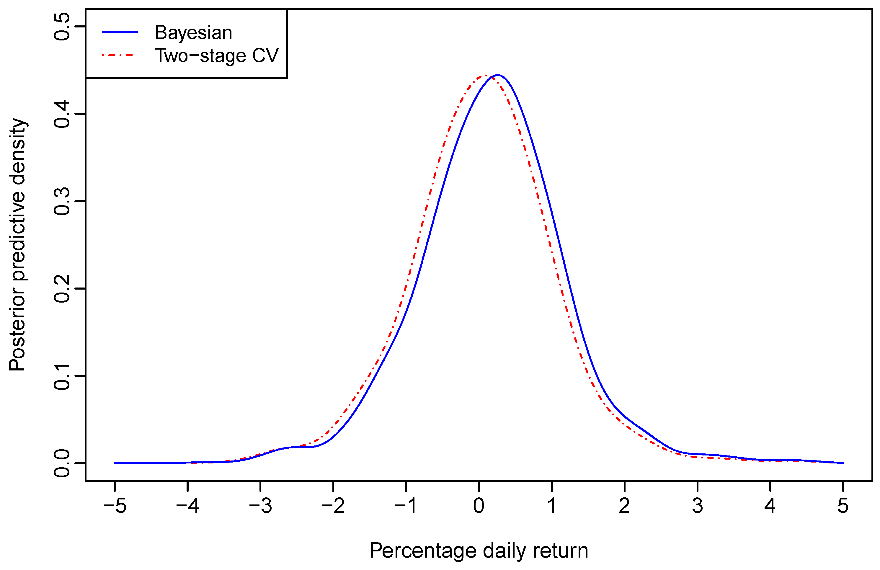
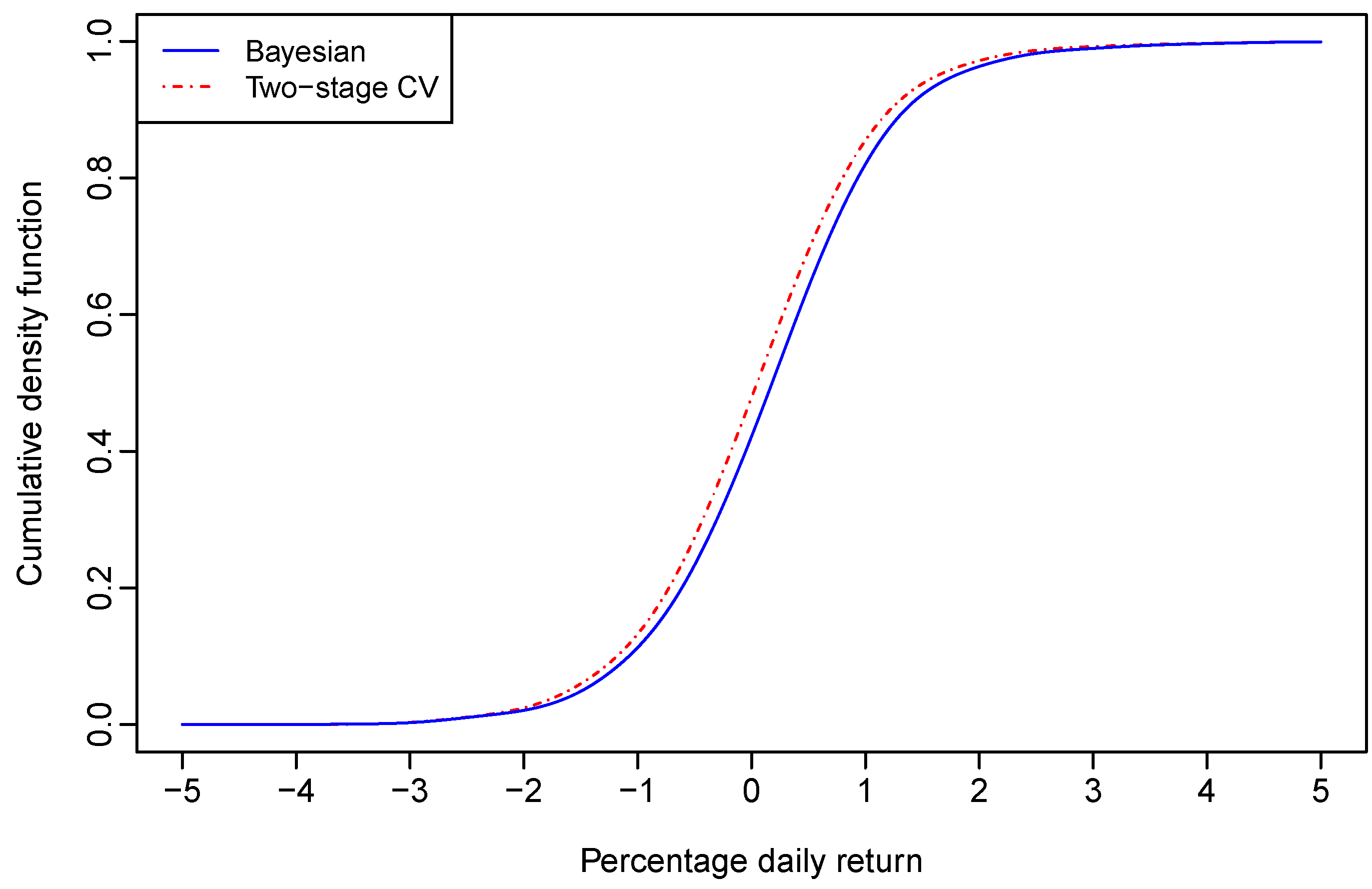
being plugged-in. Upon finishing the sampling procedure, we calculated the average of these calculated density values at each grid point. The posterior predictive cumulative density function (CDF) of the Aord daily return was obtained similarly. The posterior predictive density of the Aord return and its CDF are plotted in blue solid lines in
Figure 1 and
Figure 2, respectively.
At the 95% and 99% confidence levels, the one-day-ahead VaRs were computed through the posterior predictive CDF. With bandwidths estimated through Bayesian sampling for the nonparametric regression model given by (12), the VaRs for a $100 investment on the Aord index are respectively, $1.4861 and $2.5176 at the 95% and 99% confidence levels.
With bandwidths selected through the two–stage CV for the nonparametric regression model given by (12), the graphs of the one-day-ahead density forecast of the Aord return and its CDF are also plotted in red dot-dash lines in
Figure 1 and
Figure 2, respectively. The 95% and 99% VaRs for a $100 investment on the Aord index are respectively, $1.6048 and $2.5523, which are larger than the corresponding VaRs derived through Bayesian sampling.
It seems that the two-stage CV leads to an over-estimated VaR in comparison to its Bayesian counterpart. However, the above results were derived based on forecasted densities of one day’s Aord return only. To further justify the empirical importance of our method, we checked the relative frequency of exceedance through rolling samples.
5.3. Relative Frequency of Exceedance
The concept of exceedance refers to the phenomenon that the actual daily loss exceeds the estimated daily VaR during the same period of holding the invested asset. The relative frequency of exceedance is a measure of the accuracy of a VaR estimate. Therefore, we use this measure to evaluate the performance of the proposed Bayesian bandwidth estimation method in comparison to the two-stage CV for the nonparametric regression model with both continuous and binary regressors. The performance of the one-day-ahead forecasted VaR was examined by the relative frequency of exceedance derived through rolling samples. Let α denote the confidence level for computing VaRs. If the relative frequency of exceedance is close to , the underlying method for computing the VaR can be regarded as appropriate. The closer the relative frequency of exceedance is to , the better the underlying VaR estimation method would be.
In order to calculate the relative frequency of exceedance, the samples have a fixed size of 1000. During the whole sample period, the first sample contains the first 1000 observed vectors of the Aord, S&P 500 and FTSE returns, based on which we estimated bandwidths through Bayesian sampling and computed the VaRs at the 95% and 99% confidence levels. The second sample was derived by rolling the first sample forward one day. Based on the second sample, we did the same as for the previous sample. This procedure continued until the second last observation was included in the sample for estimating bandwidths. There are a total of 373 samples for forecasting the one-day-ahead VaRs.
With the daily VaRs forecasted through rolling samples, we calculated the relative frequency of exceedance at different α values with bandwidths chosen through Bayesian sampling and the two-stage CV. With Bayesian sampling, the resultant relative frequencies are respectively, 0.80% and 4.81% at the 99% and 95% confidence levels. However, with two-stage CV method, the corresponding relative frequencies of exceedance are 1.07% and 6.95%, respectively. It shows that two-stage CV for bandwidth selection leads to under-estimated VaRs in comparison to our proposed sampling method, particularly at the 95% confidence level.
6. Conditional Density Estimation of GDP Growth Rates
Given the close relationship between the conditional mean regression and conditional density estimation, the sampling algorithm proposed in
Section 3 can be modified for the purpose of choosing bandwidths in kernel density estimation of continuous and discrete variables. Maasoumi, Racine, and Stengos [
7] investigated kernel density estimation of the gross domestic product (GDP) growth rate among OECD and non-OECD countries from 1965 to 1995, where the OECD status of the country and the year of the observed growth rate are included in the data matrix. They aimed to estimate the trivariate density of growth rates (denoted as
), OECD status and year (denoted as
), where the last two variables are respectively, binary and ordered categorical. Their primary purpose was to explore the dynamic evolution of OECD and non-OECD countries’ distributions of GDP growth rates across different years. Maasoumi
et al. [
7] proposed using the kernel estimator with unordered and ordered discrete kernels assigned to the discrete variables to estimate such trivariate densities, where bandwidths were selected through the likelihood cross-validation (LCV) (see also [
7,
47]).
We are interested in choosing bandwidths for the kernel estimator of
, which is expressed as
where
and
, for
, are observations of
and
, respectively. The kernel function for GDP growth rates is the Gaussian kernel, while the OECD status is assigned with a kernel function given by (3), and the kernel for years is given by (4).
The likelihood of
for given
is approximately
where
is the leave–one–out version of
(see for example, [
48]).
The priors of bandwidth parameters are the same as those discussed in
Section 3.2. The posterior of
is proportional to the product of
and the priors of bandwidths. The adaptive random-walk Metropolis algorithm was used to implement the posterior simulation, where the proposal density is the standard trivariate Gaussian, and the tuning parameter was chosen to make the acceptance rate around 0.234. The posterior mean of each simulated chain is used as an estimate of the corresponding bandwidth.
With the estimated bandwidths, we derived the joint density of GDP growth rate, OECD status and years. The conditional density of GDP growth rates for given values of OECD status and year is the joint density estimator divided by the marginal density estimator of OECD status and year. Note that bandwidths estimated for the joint trivariate kernel density estimator can be used for the kernel conditional density estimator.
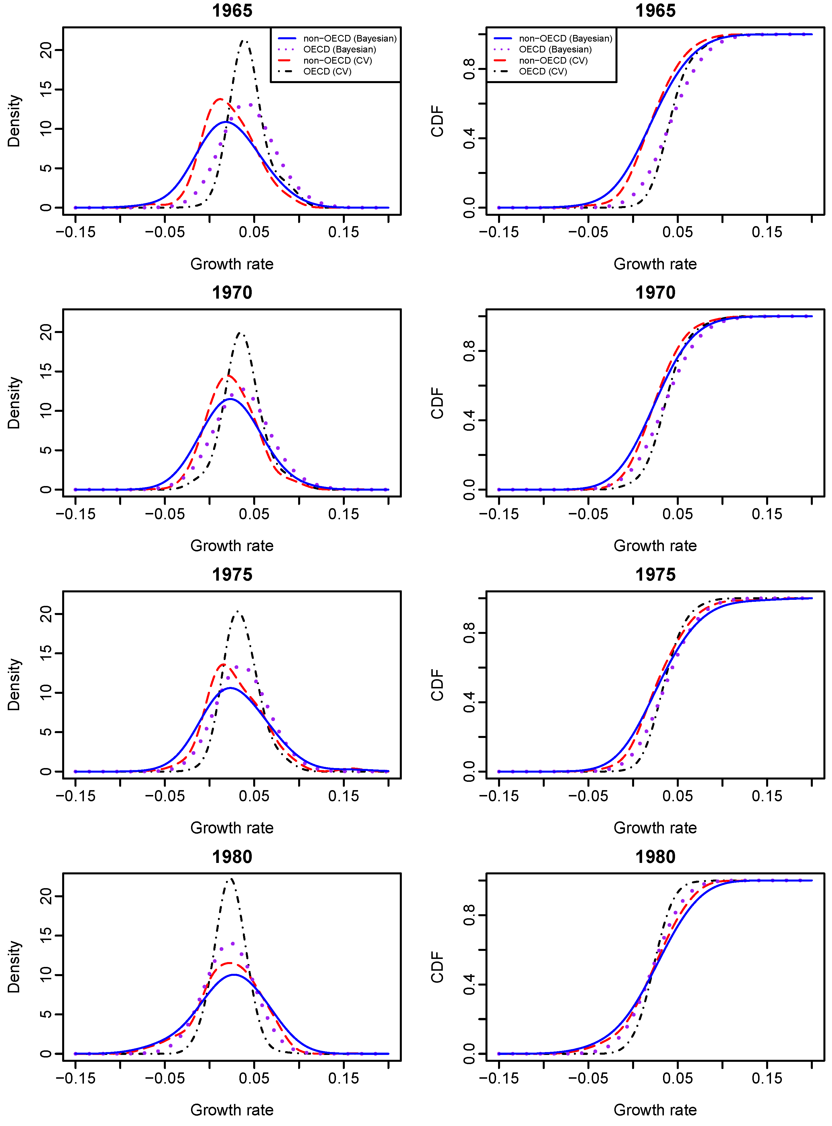
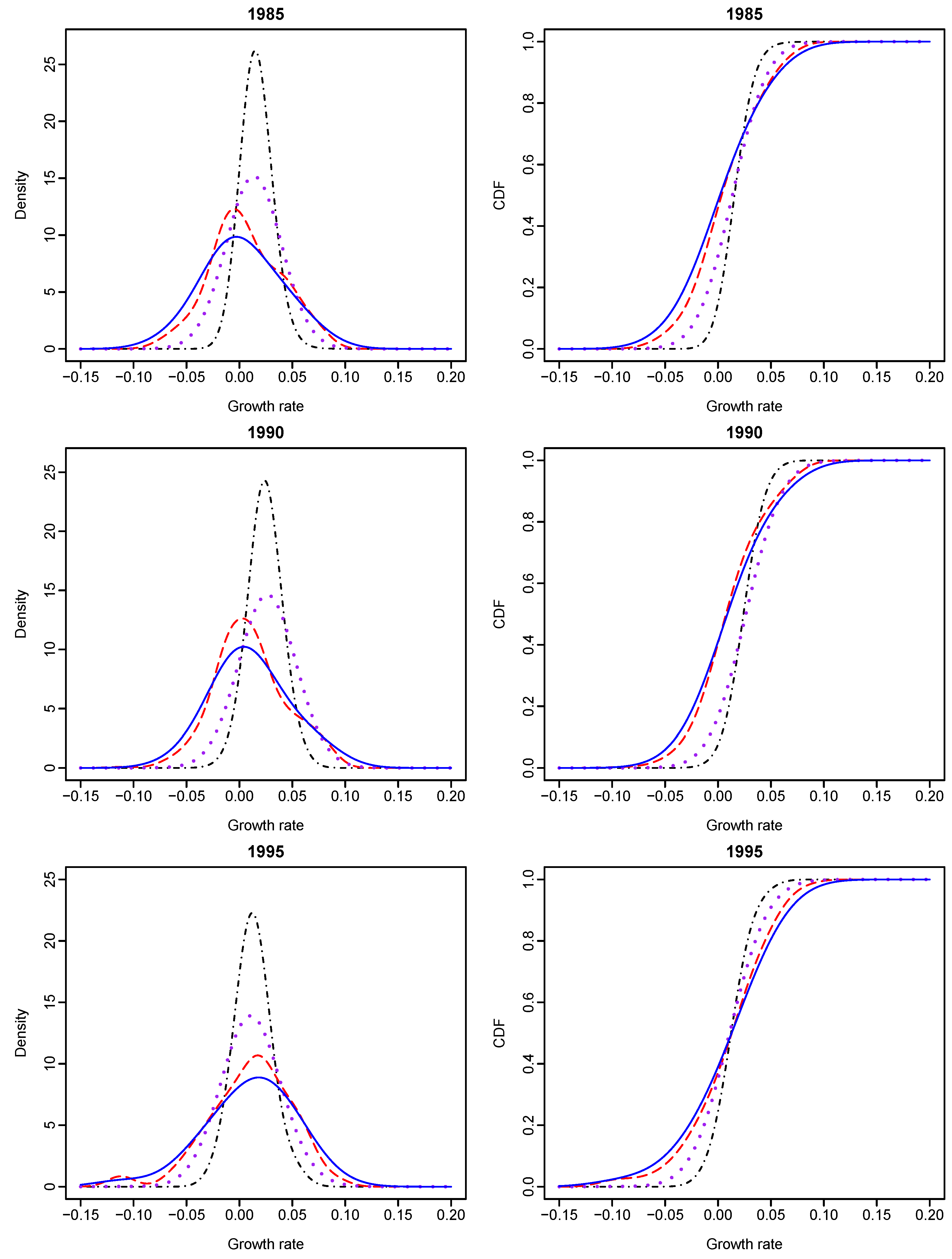
Given different values of OECD status and year, we calculated the conditional densities and CDFs of GDP growth rates with their graphs presented in
Figure 3 and
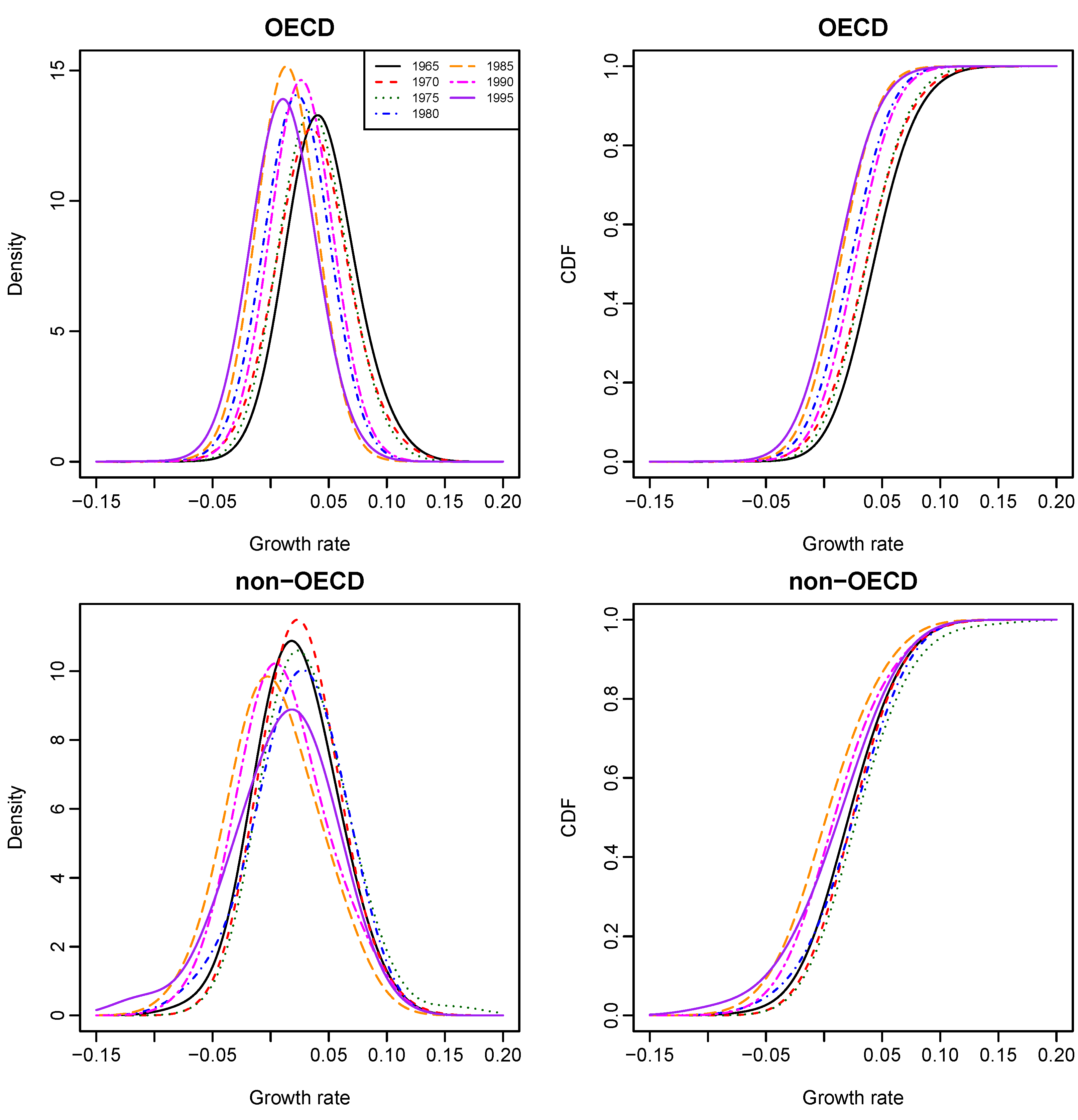
Figure 4. It shows that Bayesian sampling and LCV lead to clearly different density functions of growth rates. The probability density estimates obtained from LCV have higher peaks than those obtained from the Bayesian method, although they both center at about the same points. The growth-rate distributions of an OECD country and a non-OECD country are very different from 1965 to 1995. Second, the growth-rate density of an OECD country is almost symmetrical and less dispersed than that of a non-OECD country, and this phenomenon becomes obvious over time. The growth-rate density of a non-OECD country is asymmetrical and has larger variation than that of an OECD country. It appears to manifest bimodality and indicate “polarization” within non-OECD countries. The results re-confirm the findings of [
7].
Figure 5 presents the stacked plots of OECD and non-OECD density and distribution functions of growth rates for all years, where bandwidths were estimated through Bayesian sampling.
We found the following empirical evidence. First, given the year value at either 1965 or 1970, the conditional growth-rate distribution of an OECD country (purple dotted line on the two top right graphs of
Figure 3) stochastically dominates that of a non-OECD country (blue solid line). However, there has been no such stochastic dominance since 1975. Second, given the OECD status of a country, the country’s growth-rate distribution in 1965 (black solid line on the top right graph of
Figure 5) stochastically dominates its growth-rate distributions in the other years; and its growth-rate distribution in 1990 (pink long- and short-dashed line) stochastically dominates its growth-rate distributions in 1980 (blue dot-dash line), 1985 (brown dashed line) and 1995 (purple solid line), respectively.
7. Conclusions
We have presented a Bayesian sampling approach to the estimation of bandwidths in a nonparametric regression model with continuous and discrete regressors, where the regression function is estimated by the NW estimator and the unknown error density is approximated by a kernel-form error density. Monte Carlo simulation results show that the proposed Bayesian sampling method typically performs better than, or at least on par in only a few occasions with, cross-validation for choosing bandwidths. In particular, the Bayesian method performs better than the CV method when the sample size is small. The advantage of the proposed Bayesian approach over cross-validation is its ability to estimate the error density. As measured by the MISE, the Bayesian method outperforms the two-stage cross-validation method for estimating the bandwidth in the kernel-form error density. Thus, the proposed sampling method is recommended for estimating bandwidths in the regression-function and kernel-form error density estimators.
The proposed Bayesian sampling algorithm is used to estimate bandwidths for the nonparametric regression of All Ordinaries (Aord) daily return on the overnight S&P 500 return and an indicator of the FTSE return. In comparison to cross-validation for bandwidth selection, the proposed sampling method leads to a different one-step-ahead forecasted density of the Aord return. Consequently, the resulting value-at-risk measure, as well as the relative frequency of exceedance, is different from the one derived with bandwidths selected through cross-validation. In this example, Bayesian sampling for bandwidth estimation in the nonparametric regression of mixed regressors leads to better results than cross-validation. In an application that involves of kernel density estimation of a country’s GDP growth rate conditional on its OECD status and the year of observations, Bayesian sampling for bandwidth estimation leads to different density estimates from those with bandwidths selected through likelihood cross-validation.
There are several ways, along which this paper can be extended. First, the proposed Bayesian algorithm can be extended to several other models, one of which is the nonparametric regression model with conditional heteroscedastic errors or correlated errors. Second, it is possible to consider using asymmetric kernel functions for continuous variables, such as the beta and gamma kernels discussed by in [
45], as well as other kernels for discrete variables, such as the binomial and Poisson kernels discussed by [
44]. We leave these extensions for future research.


