Abstract
A specific concept of structural model is used as a background for discussing the structurality of its parameterization. Conditions for a structural model to be also causal are examined. Difficulties and pitfalls arising from the parameterization are analyzed. In particular, pitfalls when considering alternative parameterizations of a same model are shown to have lead to ungrounded conclusions in the literature. Discussions of observationally equivalent models related to different economic mechanisms are used to make clear the connection between an economically meaningful parameterization and an economically meaningful decomposition of a complex model. The design of economic policy is used for drawing some practical implications of the proposed analysis.
Keywords:
structural model; recursive decomposition; exogeneity; causality; model identification; observationally equivalent models; structural invariance; misleading constraints; structurality PACS:
12.40.Ee
MSC:
62F99, 62H05
JEL classification:
C10, C18, C50, C51, C54
1. Introduction
In this paper, we develop a concept of structural econometric model through a specific model building strategy and embed the concept of causality within the framework of a suitably constructed structural model, justifying accordingly that a structural model be also called a causal model. We show that the structurality of a model depends both on its probabilistic structure and on its parameterization. We also expose some difficulties, and pitfalls, in the treatment of identification and of reparameterization, particularly when treating observationally equivalent models through different parameterizations.
A structural econometric model endeavors at unfolding the structure of an underlying economic mechanism assumedly generating the observed data. In the words of Illari and Williamson [1]: “A mechanism for a phenomenon consists of entities and activities organized in such a way that they are responsible for the phenomenon”. This definition is general enough to be applicable to social contexts too. For economic phenomena, a mechanism may be viewed as a mathematical structure that models choices of economic agents or institutions through which economic activity is guided and coordinated. This mathematical structure provides a representation of a mechanism either in a deterministic form, when the model is assumed to provide a complete explanation of a phenomenon, or in a probabilistic form when the explanation is considered as an incomplete one. An econometric model refers to the second alternative and takes the form of a conditional distribution where the endogenous variable is the one generated by the mechanism and the conditioning variables are those under which the mechanism is operating.
We rely on a specific approach to structural modeling that combines, as in Mouchart, Wunsch and Russo [2], two main econometric traditions. On the one hand, one of these traditions starts from a “theory” (i.e., economic theory) and develops a structural model from the statistical implications of that economic theory. This approach has been proposed by the Cowles Commission, in particular Koopmans [3] and Haavelmo [4]. On the other hand, another stream starts from the idea of a “Data Generating Process ” (DGP), representing how the data have been generated: a structural model looks for a structure underlying the DGP. This approach has been launched by Sargan [5] at LSE and further developed by Hendry [6] and others.
The order of exposition is as follows. In the next section, we propose a statistical approach to the concept of structural model by successively examining econometric models as a class of statistical models and the recursive decomposition of a model as a device for providing explanatory power to a model. We also show that the parameterization of a decomposed model is part of the explanatory process. Section 4 presents two major difficulties occurring when treating the parameterization of a structural model. A first one deals with illegitimate constraints when blending two parameterizations of a same model. We show, in particular, that this error has been made repeatedly in the econometric literature. Another difficulty deals with the structural interpretation of the parameterizations of two different economic mechanisms leading nevertheless to observationally equivalent models. The last section takes an helicopter view of the achievements of this paper and points out, in particular, some implications for the design of an economic policy based on an econometric model.
2. Structural Econometric Modeling: A Specific Approach
2.1. Econometric Models as Statistical Models
In this paper, we approach an econometric model as a particular type of statistical model.
Formally, a statistical model may be viewed as a set of probability distributions, explicitly:
where S, the sample space or observation space, is the range space of an observable random variable (or vector of variables) and for each , is a probability distribution on the sample space, i.e., the sampling distribution. In other words, ω is a characteristic, or parameter, of the corresponding distribution and Ω describes the set of all sampling distributions belonging to the model. The basic idea is that the data are to be analyzed as if they were a realization of one of those distributions. A statistical model can accordingly be viewed as a set of plausible hypotheses regarding the Data Generating Process (for short, DGP); for an historical perspective, see Haavelmo [7] and Zellner [8] and for quite an interesting updating see e.g. Hendry [9].
A statistical model is based on a stochastic representation of the world. The random component of the model delineates the frontier, or the internal limitation, of the statistical explanation. More explicitly, the randomness represents what is not explained by the model, while the parameters of the distributions are the cornerstone of the statistical explanation.
2.2. Recursive Decomposition
An econometric model is not always structural. Its aim may be to provide an insightful description of the observed data without the ambition of unfolding the mechanisms and sub-mechanisms underlying the DGP. Thus, many macro-econometric models as well as models of financial econometrics are based on the literature concerning the empirical issue of interest and on some stylized facts that the author aims to interpret. These models are of a descriptive nature, as they do not aim at unfolding a structural mechanism underlying a DGP.
A structural econometric model is not only aimed at providing a stochastic representation of a global mechanism, but should also provide an explanation of that process. Once the model is dealing with a large number of variables, the usual way of explaining a complex process is given by a decomposition of the global mechanism into an (ordered) sequence of simpler sub-mechanisms. This is the objective of a recursive decomposition of a statistical model.
More explicitly, let us consider a partition of the vector X into p components: . Suppose that the components of X have been ordered in such a way that in the complete marginal-conditional decomposition of the joint distribution of X:
each component of the right hand side is characterized by mutually independent parameters, i.e., variation-free in a sampling theory framework:
or a priori independent in a Bayesian framework. When each factor in (2) stands for a univariate conditional distribution, Equations (2) and (3) characterize a completely recursive system. When some, or all, factors represent the conditional distribution of a vector of variables, Equations (2) and (3) characterize a partially recursive, or block-recursive, system.
The right-hand side of Equation (2) may be interpreted as an ordered sequence of p sub-mechanisms, each one characterized by a distribution generating a variable conditionally on (an increasing set of ) conditioning variables. This is in line with Illari and Williamson [1] and is compatible with an interpretation of the recursive decomposition in terms of sub-mechanisms in a structural model, as detailed in Wunsch, Mouchart and Russo [10]. Equation (3) requires that there are no restrictions binding the parameters of different factors of (2), in particular that there are no common parameters, and allows one to interpret each factor of the decomposition as independent sub-mechanism.
A reference to the Simultaneous Equations Model (SEM) may be useful. In its standard formulation, the structural form of the SEM may be written as follows.
Condition implies that the equation in (4) is derived from the conditional distribution of and its conditional expectation is given by the reduced form:
This model is said recursive when the matrix B is lower triangular (along with the usual normalization rule of making the elements of the main diagonal equal to 1) and Σ is diagonal. Under a normality assumption, this recursive system of equations stands for an ordered sequence of conditional expectations and errors are mutually independent. In this case, the SEM corresponds to a completely recursive decomposition of the joint distribution of the endogenous variables y conditionally on the exogenous variables z and the global mechanism generating is “explained” through an ordered sequence of sub-mechanisms represented by an ordered sequence of conditional univariate distributions.
When the SEM is not recursive, Equation (4) does not refer to conditional distributions, does not stand for conditional expectations (along with errors) and may be interpreted as referring to “notional” sub-mechanisms in a spirit similar to that of counterfactuals. For instance, consider a two-equations elementary market model, generating price and quantity under a competitive equilibrium. The equation representing the quantity demanded as a function of the price and other exogenous variables, may be interpreted as the notional demand that would operate if the prices were exogenously fixed whereas the econometric model specifies that the actually observed prices, and quantities, have been jointly generated under an equilibrium mechanism.
From a causality point of view, Equation (5) reflects a situation of block-recursivity: a global mechanism “explains” that vector z “causes” vector y but no explanation is given about the functioning of that mechanism. Only if model (4) were recursive would one obtain an explanation of the functioning of that global mechanism through a causal ordering in terms of sub-mechanisms.
2.3. Recursive Decomposition: Explanation and Structurality
In this section, we endeavor to make the concept of structurality of an econometric model more precise and specific. The recursive decomposition provides a structure for the explanation of a complex system through an ordered sequence of sub-mechanisms that compose the global mechanism. However, conditions (2) and (3) are not sufficient for ensuring that a given recursive decomposition is the valid one among the possible recursive decompositions (corresponding to the number of ordered permutations of p variables). We also require conditions for ensuring that each factor of the product in (2) represents a valid sub-mechanism.
The required conditions are twofold. Firstly, each putative sub-mechanism, represented by a specific conditional distribution, should be congruent with field knowledge, i.e., with economic theory, as long as this one may be viewed as an organized synthesis of a large body of out-of-sample observations relative to the phenomenon of interest.
Secondly, the putative sub-mechanism should be stable, or invariant, relatively to a large class of interventions or of modifications of the environment. Indeed, a conditional distribution that would be different, say, for each observation could not be deemed to represent an underlying structure neither would it be useful, at least for accumulating empirical information. This refers to the fundamental issue of defining a “population of reference”; indeed neither an economic theory nor an econometric model may reasonably claim to be “universal” in time and in space. The stability requirement concerns both the structure of the model, i.e., the recursive decomposition as a set of sub-mechanisms (see for instance Richard [11] for a change of exogeneity), and the characteristic of the sub-mechanisms, i.e., the parameters, see for instance Hendry and Mizon [12].
The structurality of the model is related to field knowledge, in particular under some form of economic theory, and to properties of stability, or invariance, with respect to a class of interventions or of changes of the environment.
When elaborating an economic policy on the basis of an econometric model, the structural validity of the model is crucial, in particular because descriptive or non-structural models would provide unreliable forecasts or policy evaluations. This criticism is known in the literature as Lucas critique (Lucas [13]), the essence of which is well summed up in this sentence: “ ... given that the structure of an econometric model consists of optimal decision rules of economic agents, and that optimal decision rules vary systematically with changes in the structure of series relevant to the decision maker, it follows that any change in policy will systematically alter the structure of econometric models ” (Lucas [13], p. 41). It is worth noting that this criticism has strongly encouraged the structural approach in macroeconometric modeling.
More generally, the issue of invariant parametrization may be particularly complex. Indeed, the characteristics, or parameters, of a conditional distribution stand for the characteristics of an economically meaningful sub-mechanism. The tradition in economic theory is to view actual behaviors as a result of an optimization process. A substantial difficulty may be to decide what, in that optimization, is actually exogenous, i.e., considered as given.
To take a simple example, when optimizing a consumption plan under a budget constraint, this assumes that the level of income has been exogenously fixed, maybe under some equilibrium with respect to leisure and opportunity to increase disposable income (see e.g., Deaton [14]. Endogenizing this process substantially increases the complexity of the model and should therefore be operated only when necessary for a correct specification of the model. If the endogenization of income is not operated in cases where it should have been, the price to be paid is not only a loss of consistency of the estimator but also a loss of stability of the the underlying parameters being actually estimated. As a matter of fact, building a model involves not only an empirical check on the parametric stability, by means for instance of hypothesis testing, but also a substantial amount of field knowledge that possibly could point out toward relevant changes of environment.
It may be interesting to notice that Heckman and Vytlacil [15], among a substantial number of publications, propose a different view on structural modeling, see also Heckman [16,17]. Compared with the above summary, Heckman and Vytlacil [15] also make use of field knowledge, in the form of an economic theory, but with a limited view on stability or invariance, through a policy-based approach, therefore in the lines of Lucas’ criticism. In this paper, this later aspect also encompasses historical and spatial aspects making of this one the cornerstones of the concept of structurality, through the concept of population of reference. Moreover in this paper, the aspect of representation is only part of the story: explanation of the functioning of the global mechanism, by means of a recursive decomposition is also crucial. Representing a complex process without explaining its functioning is not viewed as satisfactory.
Summarizing, the specific approach to structural modeling is essentially a specific strategy of model building. The structural approach blends two components. Firstly it looks for a model congruent with the field knowledge, in particular with economic theory, and stable enough, or invariant, with respect to a suitable class of interventions and of changes of the environment. In a sense it provides a representation of a global mechanism that operates a distinction between structural aspects and incidental aspects of economic reality. Secondly it also provides an explanation of the functioning of the economic world by means of a recursive decomposition of the global mechanism in terms of an ordered sequence of sub-mechanisms.
2.4. Parsimonious Modelling
Consider now a conditional distribution, say
identified as representing a plausible sub-mechanism. As a matter of fact, field knowledge, or a formal test of hypothesis, often suggests that not all conditioning variables are actually active in that sub-mechanism. More precisely, there may be a subset of the conditioning variables, or of functions of the conditioning variables, say , such that:
may be called the information set relevant for the j-th sub-mechanism, although more formally it is a σ-field rather than a set of variables. Under condition (7), the product in (2) is condensed into:
where stands for an initial condition. Equation (8) may be called a condensed recursive form and represents the actually relevant structure of the global mechanism, see also Mouchart and Russo [18].
2.5. Causal and Structural Models
When the conditions summarized at the end of Section 2.3 are satisfied, the following properties are derived: (i) The conditioning variables entering the information set may be viewed as exogenous and the conditioned variables may be viewed as endogenous, for that specific sub-mechanism. Thus, a particular variable is not endogenous or exogenous in itself, but relatively to a particular sub-mechanism; (ii) The conditioning variables may also be viewed as jointly the endogenous variable, viewed as an outcome (or, effect) variable; the corresponding conditional distribution provides a characterization of the direct effect of the cause on the outcome; (iii) The model may accordingly be called structural or ; (iv) The global mechanism may be represented graphically by means of a (for short, DAG) (for an introduction to DAG, see for instance, Pearl [19]), although the specification of the information sets and of the condensed recursive form are often out of the scope of a DAG.
The topic of causality has received a considerable attention in the literature, see e.g., Richard [20], Rubin [21] and, more recently, Imbens and Rubin [22]. This is not the place for a comprehensive summary of a large number of publications. Let us only mention that in a recent paper Heckman and Pinto [23] revisit the notions of Haavelmo’s causality adopting a recursive approach that allows to represent causal models through the Pearl’s mathematical Language of DAG. At the same time the authors point out the limitations of this approach for what concerns the econometric identification.
Remark.
It is worth mentioning that the concept of exogeneity has a long history in econometrics. The works of the Cowles Commission in the late Forties and the early Fifties have been path-breaking and are still influential nowadays; in particular, Koopmans [3] puts emphasis on exogeneity in dynamic models. Later, Barndorff-Nielsen [24], in a purely statistical framework, developed general conditions for the separation of inference, introducing the concept of a cut in a statistical model. Florens, Mouchart and Rolin [25] and Florens and Mouchart [26] bridge Koopmans and Barndorff-Nielsen works and provide a coherent account of exogeneity integrating the separation of inference in dynamic and in non-dynamic models. Engle, Hendry and Richard [27] present a classification of different concepts of exogeneity met in the econometric literature and display their connections with exogeneity through the introduction of supplementary conditions. Florens and Mouchart [26] not only provide a basic concept of exogeneity, but also make the concept explicit in different levels of model specification, namely, global, initial, and sequential, before combining those concepts of exogeneity with non-causality. This analysis is further developed in Florens, Mouchart and Rolin [28].
3. Structural Model and Parameterization
Let us now consider how to build a structural econometric model, i.e., a statistical model that would be an appropriate representation of a (global) economic mechanism in such a way that it would also provide an explanation of the working of that global mechanism. In Section 2.2, it has been mentioned that a natural strategy for enhancing the understanding of a complex multivariate mechanism would decompose that mechanism into an ordered sequence of simpler sub-mechanisms: this is the objective of the recursive decomposition. Therefore a first requirement is that each factor of the recursive decomposition should provide a suitable representation of a sub-mechanism stated in the form of a conditional distribution.
From a strictly statistical point of view, Model (1) admits any arbitrary parameterization; in other words a parameterization is just a labeling system for a set of distributions. From a structural point of view, the parameterization labels an ordered sequence of conditional distributions, in the form of (2) or (8), each one representing a structurally relevant sub-mechanism. Thus a structural parameterization is endowed with an interpretation bound to the explanation of the global mechanism and of its constituting sub-mechanisms; it is also endowed with a stability property that ensures the structurality of the parameterization and allows for the accumulation of statistical information.
These ideas may be illustrated by the following simple example. Consider a model representing a market where y stands for the price of a given commodity and z for the quantity and assume that conditionally on the past up to time , namely , the bivariate model is constructed as follows:
This model is equivalent to:
and also equivalent to:
under some obvious relationships among these different parameterizations, such as:
Let us now assume that the model aims at representing the working of a monopolistic market where the offer sets the price y under a possibly unstable process whereas the demand, generating the quantity z, is just price-taking under a stable mechanism depending only on the current price. This economic structure is captured by Model (9), the parameters of which explain the operation of the global mechanism in terms of two economically meaningful sub-mechanisms. Model (10), although statistically equivalent, does not provide an adequate structure of the global mechanism and its parameterization has no interpretation in terms of the functioning of the global mechanism. Model (11) suffers from the same weakness of explanatory power as Model (10): the factors of that underlying recursive decomposition do not represent the assumed economic structure. Moreover, Model (9) has extracted from the apparent instability of the global process some stable, and accordingly structural, parameters that are therefore estimable and succeed in isolating what is not stable. This is a simple example of the nature of structural modeling: identify relevant sub-mechanisms and uncover the stable aspects of the working of economic mechanisms.
Conversely if it is assumed that price y and quantity z are fixed simultaneously following a competitive process aiming at clearing the market, the economic structures represented by Models (9) and (11) are not valid representations of the economic structure. Only the global mechanism (10) provides a correct representation of the system without, however, having the possibility to decompose it into a sequence of simpler sub-mechanisms, i.e., without providing an explanation of the equilibrium mechanism. More explicitly, it might be possible to introduce two notional concepts of offer and demand but these concepts would not be sufficient for providing an ordered causal structure representing the functioning of the global process of competitive equilibrium.
Remark.
The recursive decomposition does not require neither a specification of the coordinates coding the variables nor a specification of a particular family of distribution. In other words, the recursive decomposition is non-parametric and is σ-algebraic in nature. The next step of the modeling is to, simultaneously, specify the coordinates of the variables and a parametrization of a chosen family of distributions.
4. Pitfalls with Alternative Parameterizations
Previous sections handle the specification and the parametrization of structural models. In a purely statistical approach, a parameterization of a statistical model is a labeling system for the distributions the set of which specifies the model.
In a structural econometric model, the parameterization is the basis for the explanatory mission of the structural model, provided the parameterization bears on a structurally valid recursive decomposition.
In this section, we treat some difficulties, and possible pitfalls, when facing alternative possible parameterizations. These issues are indeed important for a proper understanding of what is at stake with the choice of the parameterization. We shall discuss two different questions. The first one is exemplified with a case of simultaneous equations. Two parameterizations are used for estimation purposes: the structural form and the reduced form. Restrictions on the structural form ensure the identification of the parameters characterizing the notional concepts underlying the equations of the structural form; the proper relationship between the two parameterizations has however been the object of repeated misunderstandings in the econometric literature. A second type of problems is raised when different structural models are observationally equivalent, i.e., correspond to a same statistical model, namely a same set of distributions. This is a matter of model identification, as different from parametric identification.
4.1. Reparameterizations Suggesting Erroneous Constraints
4.1.1. A Simple Pedagogic Example
Consider the following assertion: “In a univariate normal distribution, , if the variance tends to zero, the expectation μ necessarily tends to zero”. As a “ proof”, of this assertion, consider the inverse of the coefficient of variation ; thus and therefore implies .
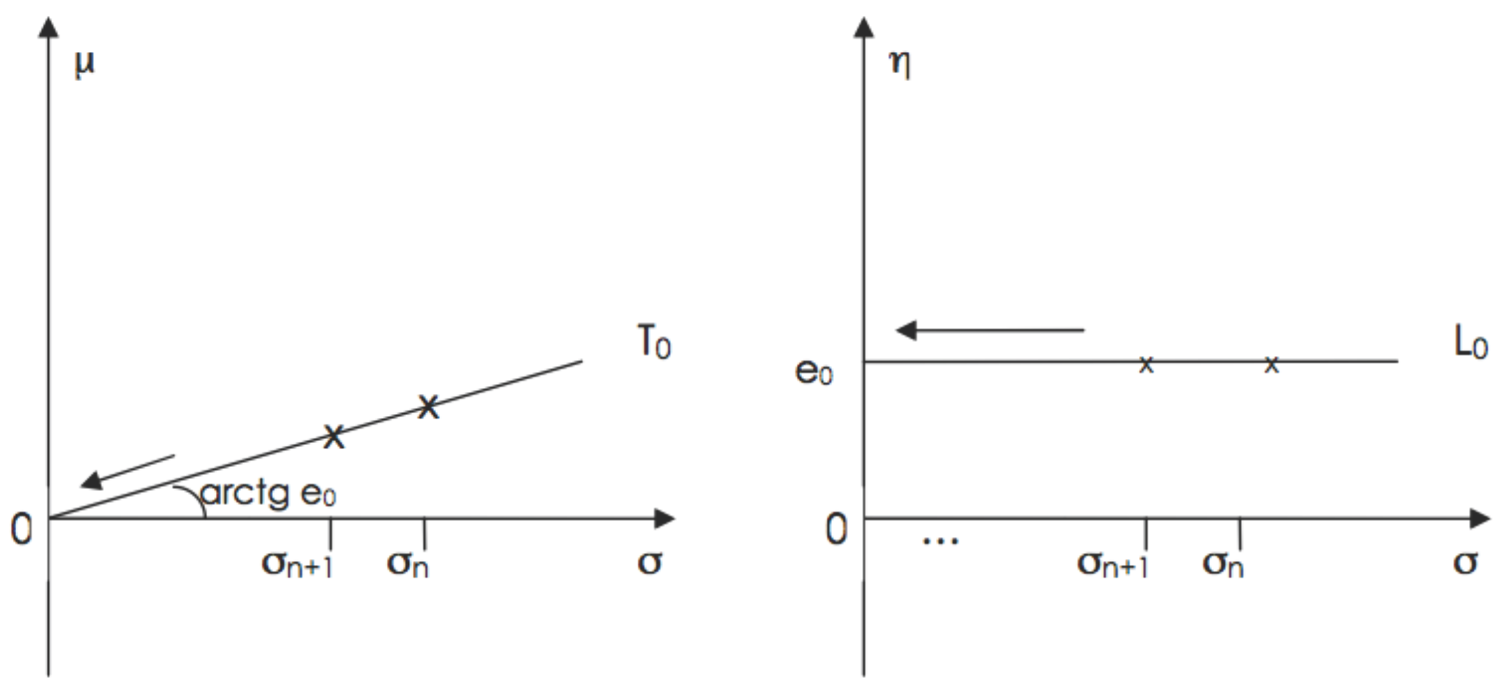
Such an assertion and its “proof” rest on a fallacious argument. The error may be viewed as follows: the pair gives one parametrization of the univariate normal family while gives another one; both parameterizations (of the same family of distributions) have the same parameter space without restrictions on the range of variation of the parameters. The argument “ implies ” is therefore invalid because it is based on a relationship () involving two different parameterizations: and . The fallaciousness of the assertion above may be viewed graphically in Figure 1 as follows. Let us consider a fixed value of η and the corresponding subsets of the two parametrizations and . Clearly and correspond to each other: they represent the same set of normal distributions. To a converging sequence corresponds, in , a sequence converging to and, in , a sequence converging to . This trivial fact does not imply any relationship between μ and σ in Θ, i.e., Θ has a product structure, equivalently μ and σ are variation-free.

Figure 1.
A same converging sequence in two parameterizations.
4.1.2. A Case in Simultaneous Equations
As naive as it may seem, the previous fallacious argument has been met in less elementary situations, when considering different parameterizations of a given model. As an example, let us consider the simplest version of Haavelmo’s [4] model:
with reduced form:
where , , . Let us also assume that independently of (or of ). The reduced form implies and therefore . This (true) inequality appears to have been erroneously interpreted as a constraint on the parameter space. For instance, Genberg [29] suggests to estimate α under the restriction , where q would be a consistent estimator of the variance ratio and notices that if one were to use a ratio of sample moments to estimate the restriction would not be binding when estimating α by ordinary least squares. Remark that Gensberg’s proposal could also be used to assert that Haavelmo’s model implies a (wrong) restriction over , namely .
As a matter of fact, we have two parameterizations (structural form and reduced form) of a same model, namely , say and , say. These parameterizations are in bijection and each is variation-free: there is no constraint among the parameters within a same parameterization. The variance of y, , is a function of these parameters, indifferently of θ or of λ, it is not a new parameter and introduces no new constraint neither on θ nor on λ. In particular, the (true) inequality does not introduce a constraint within the parametrization θ1.
In order to ascertain how fallacious these arguments of “constraints often overlooked”—see Zellner [30,31,32] and Maddala [33,34]—are, we consider, in rather obvious notation, two equivalent parameterizations of the set of bivariate normal distributions on :
where , , and is the cone of the (Semi Positive Definite Symmetric, i.e., and ) matrices. It should be pointed out that there is no restriction on the range of α, neither on that of nor on that of . As in the pedagogic example, inequalities like involve two different parameterizations and represent no restriction on any parameter space.
Before qualifying the use of such inequalities as misleading restrictions, it may be illustrative to consider a slightly more general version of the very same example. Let us consider the model:
where is a matrix the elements of which are known functions of a vector of unknown parameters α. This model may also be written as:
where . Thus we consider two equivalent parametrizations:
where A is the set of possible values for α, the “free” parameters of the (possibly overidentified) reduced form. Here it is valid to recognize that the parameter space is restricted by the condition: , i.e. should be , and thus are not variation free . Note however that the relationship , although true, does not provide any effective restriction as it grounds on two different parametrizations. The danger of overlooking this fact can be illustrated in the particular case where with and . Thus, in this particular case:
Here it is valid that, in , parameters and should be restricted by:
or, more explicitly:
(Note that one of the first two inequalities is redundant). A fallacious use of the (true) relationship would be to assert that, from the above inequalities, γ is constrained to satisfy restrictions such as the following ones:
In other words, we disagree with the assertion that (21) or (22) would mean that “certain parameter values are subject to bounds flowing from usual specifying assumptions” (Zellner [30], p. 852). Indeed Inequalities (21) and (22) do not represent restrictions neither on nor on : they only express some properties of the correspondence between and . As a consequence, estimating γ, for instance, under the restriction implied by consistent estimates of the bounds of Inequalities (21) would either be ineffective, if a correct parameterization is employed, or would consist of using twice the same sample information if one were to step from one parameterization to another one. This later would be the case when estimating e.g., bounds in one parameterization before estimating the other parameterization without taking due account of the double use of the same sample information.
When pooling two sources of information as is done with Bayesian methods or in pooling time series and cross-section data or in mixed estimation, the use of two parameterizations may be justifiable. In the above example, while may be the most natural parameterization for the final inference, it may be that some prior informations on, say, are available, leading to consider also the parameterization as a natural recipient for that prior information. If inference only concerns parameters common to and , i.e., α and/or , one may also start by first incorporating the prior information in the -parameterization and thereafter reparameterize in before incorporating the second information. Such a stepwise procedure seems to be the only available one in the case of inference on . It should nevertheless be noticed that even in such a case Inequalities (21) or (22) will never appear as restriction on any parameter space.
The reader may like to compare this analysis with the debate between Maddala [33,34] and Zellner [30,31,32] that has been inconclusive for missing the issue of the relationships between alternative parameterizations.
4.2. Reparameterizations Involving Different but Observationally Equivalent Sub-Mechanisms
The previous section illustrates possible abuse of restrictions due to a fallacious argument involving alternative parameterizations. In this section, we consider two different structural models that are nevertheless observationally equivalent and, therefore, correspond to two different parameterizations of a same model. In such cases the two parameterizations correspond to two different (sub-)mechanisms possibly suggesting different contextually relevant parametric restrictions. As a matter of fact the price equations of the two models below represent two structurally different mechanisms, and the corresponding parameters capture quite different economic meanings.
Consider a simple price adjustment model (from Bowden [35]):
where (demand), (supply) and (price) are endogenous variables, and are exogenous variables and is a “clearing” price defined as:
Therefore, the reduced form of the price equation is:
Consider another model (from Fair and Jaffee [36]) given by Equations (23) and (24) and the alternative specification of the price adjustment mechanism
equivalently:
Therefore, the reduced form of the price equation is:
Notice that (25) has sense only if whereas in (28) one should require . Therefore the parameter spaces corresponding to these two price adjustment models are:
where is the number of variables in , is the number of variables in (for the sake of presentation, we assume no common exogenous variable in and ), and .
The two price Equations (25), along with (27) and (28) with (30), represent two different sub-mechanisms. These two models are nevertheless observationally equivalent because they provide two different parameterizations of a same set of distributions. Indeed, from the coefficients of the mapping between θ and λ is given by:
implying that in Equations (31) and (32) we indeed have:
Moreover, for the coefficients of , we may check that:
and conclude that the two models are observationally equivalent under the identification relationship:
As a matter of fact, Equation (34) may be viewed as a short-hand notation for:
Note that μ and Σ are variation free in Θ; so are also η and in Λ. It may be nevertheless tempting to erroneously conclude from (34), as in the previous section, that “ implies because ”.
Once the two models are recognized as observationally equivalent, does it imply that the two price sub-mechanisms are also equivalent? The answer is: no! Indeed, Equations (25) and (28) explain the disequilibrium of the market by two different price sub-mechanisms: in Equation (25) the price sub-mechanism partially adjusts the past price to the current equilibrium price whereas Equation (28) partially adjusts the past price in function of the disequilibrium in quantity. Thus parameters μ and η have a clearly different economic meaning. In other words, the choice between the specifications of these two models is a choice between two different parameterizations of a same (conditional) distribution and should be based on economic and contextual plausibility and on structural stability.
The example above illustrates several issues. Firstly, the two models are observationally equivalent: no data may decide in favor of one against the other. Nevertheless, the two price equations represent two structurally different sub-mechanisms, the corresponding parameters being endowed with quite a different economic meaning: only field knowledge, structural stability (or invariance) or new information may decide which one is actually structural. Secondly, again, one should operate a clear distinction between relationships among alternative parameterizations, bringing no restrictions on the parameter space, and genuine restrictions that might be used either to improve inference, if accepted, or to be subjected to testing, if put in doubt. Thirdly, alternative parameterizations may possibly bring interesting information in an encompassing spirit. For instance, if one is willing to interpret the parameters of Bowden’s model at the light of Fair and Jaffee’s model, relationship (33) would tell that a value of μ close to 0 (resp. 1) in the first model would correspond to a great (resp. small) value of η in the second model. But this relationship implies no restriction neither on μ nor on η.
More recently, An and Schorfheide [37] produced another example of two observationally equivalent models corresponding to two different parameterizations of a same family of conditional distributions. These two models describe different sub-mechanisms characterized by parameters with a different economic interpretation. Through an implied identification problem, they propose to work out a Bayesian solution. This example shows that when specifying a structural model it is not sufficient to specify a family of distributions: a particular parameterization, with a specific economic meaning, should also be specified.
5. Concluding Remarks
5.1. Summarizing: The Basic Framework
In this paper, we make explicit the link between causal model and structural model. In particular, the structural explanation of a model is based on a recursive decomposition of the model itself, together with the interpretation of each term of the structural decomposition as an economic sub-mechanism. When we can reach this model structuring, the explanatory variables can be interpreted as causal variables.
We also propose an approach for building a structural econometric model, i.e., a statistical model that provides (i) an appropriate representation of a global economic mechanism and (ii) an explanation of the working of that global mechanism i.e., each factor of the recursive decomposition should provide a suitable representation of an economically meaningful sub-mechanism.
The necessary conditions for a recursive decomposition to be interpreted as a structural model, are: (i) there is congruence with the underlying economic theory (ii) there is invariance or stability of the parameters characterizing the economic sub-mechanisms as well as of the recursive decomposition itself.
One limitation of this approach is that the explanatory power of the model relies on its recursive decomposition. A completely recursive decomposition provides a complete causal ordering of the variables. When a completely recursive decomposition is not possible, i.e., the case of block-recursivity where the recursive decomposition is only partial, there is a simultaneity of the action of several sub-mechanisms within the generation of a block of endogenous variables. In this case, the model cannot claim for causal effects within the block of endogenous variables because outcomes cannot cause each other simultaneously.
From a narrow statistical point of view, the parameterization of a family of distributions is arbitrary. In a structural modeling approach the issue is more subtle. Indeed, a basic requirement of structurality is the stability of the recursive decomposition, involving both the stability of the decomposition itself and the stability of the parameters of the different distributions. As a matter of fact, the stability of these characteristics is, in general, not complete. As mentioned in an example of Section 3, some factors of the decomposition may be more stable than others. Therefore the specification of the parameterization should be based on the search of the parameters that are likely to be more stable; this ensures that these parameters are endowed with a reliable economic meaning.
This paper also makes explicit some difficulties and pitfalls when handling alternative parameterizations, namely the danger of introducing illegitimate constraints in case of alternative parameterizations of a same model, or selecting among two different sub-mechanisms leading to observationally equivalent models.
5.2. On the Use of Models for the Design of Economic Policy
An intervention, such as an economic policy, should be based on a structural, or causal, model rather than on a descriptive model. More specifically, econometric models used for the design of economic policy should represent actual behavior, be it macro or micro, rather than provide a representation based on theoretically grounded behavior. This is precisely the meaning of an econometric structural, or causal, model.
Thus the model builder should carefully check the structural stability of the model, in particular its resilience to a suitable class of transformations of the environment. Indeed the parameters and the recursive structure of the model should not be thought in a universal sense, in space and in time, and it is crucial to evaluate how the “universe” should be circumscribed. Lucas’ critique may indeed be interpreted as referring to the fact that an intervention may modify the structure of the causal model, because a model is developed within a given environment and the difficulty may be to evaluate to what extent a modification of the environment might modify some properties of the causal model. Thus the strategy for building an econometric model should identify the relevant sub-mechanisms from the apparent instability of the global process and the stable aspects of the working of economic mechanisms.
Author Contributions
This paper is a result of a joint work where each author had an equal contribution.
Conflicts of Interest
The authors declare no conflict of interest.
References
- P.M. Illari, and J. Williamson. “What is a mechanism? Thinking about mechanisms across the sciences.” Eur. J. Philos. Sci. 2 (2012): 119–135. [Google Scholar] [CrossRef]
- M. Mouchart, G. Wunsch, and F. Russo. “The issue of control in multivariate systems: A contribution of structural modelling.” Available online: http://dial.uclouvain.be/handle/boreal:162165?sit_ename=UCL (accessed on 7 April 2016).
- T.C. Koopmans. “When is an Equation System Complete for Statistical Purposes? ” In Statistical Inference in Dynamic Economic Models. Edited by T.C. Koopmans. Cowles Commission Monograph 10; New York, NY, USA: John Wiley & Sons, 1950. [Google Scholar]
- T. Haavelmo. “Methods of measuring the marginal propensity to consume.” J. Am. Stat. Assoc. 42 (1947): 105–122. [Google Scholar] [CrossRef]
- J.D. Sargan. “Wages and Prices in the United Kingdom: A Study in Econometric Methodology, (with Discussion).” In Econometric Analysis for National Economic Planning. Edited by P.E. Hart, G. Mills and J.K. Whitaker. London, UK: Butterworth, 1964, Volume 16, pp. 25–63. [Google Scholar] Reprinted in Econometrics and Quantitative Economics. D.F. Hendry, and K.F Wallis, eds. Oxford, UK: Blackwel, 1984. and in Contribution to Econometrics. J.D. Sargan, ed. Cambridge, UK: Cambridge Univesity Press, 1988, Volume 1.
- D.F. Hendry. “Econometric Methodology: A Personal Perspective.” In Advances in Econometrics. Edited by T.F. Bewley. Cambridge, UK: Cambridge Univesity Press, 1987. [Google Scholar]
- T. Haavelmo. “The Probability Approach in Econometrics.” Econometrica 12 (1944): 1–118. [Google Scholar] [CrossRef]
- A. Zellner. “Statistical Analysis of Econometric Models.” J. Am. Stat. Assoc. 74 (1979): 628–643. [Google Scholar] [CrossRef]
- D.F. Hendry. Dynamic Econometrics. Oxford, UK: Oxford University Press, 1995. [Google Scholar]
- G. Wunsch, M. Mouchart, and F. Russo. “Functions and mechanisms in structural-modelling explanations.” J. Gen. Philos. Sci. 45 (2014): 187–208. [Google Scholar] [CrossRef]
- J.-F. Richard. “Models with several regimes and changes in exogeneity.” Rev. Econ. Stud. 47 (1980): 1–20. [Google Scholar] [CrossRef]
- D.F. Hendry, and G.E. Mizon. “Exogoneity, causality, and co-breaking in economic policy analysis of a small econometric model of money in the UK.” Empir. Econ. 23 (1998): 267–294. [Google Scholar] [CrossRef]
- R. Lucas. “Econometric Policy Evaluation: A Critique.” In The Phillips Curve and Labour Markets. Edited by K. Bruner and A. Metzler. Carnegie-Rochester Conference Series on Public Policy; New York, NY, USA: American Elsevier, 1976, Volume 1, pp. 19–46. [Google Scholar]
- A.S. Deaton. “Model Selection Procedures, or, does the Consumption Function Exist? ” In Evaluating the Reliability of Macro-Economic Models. Edited by G.C. Chow and P. Corsi. New York, NY, USA: John Wiley and Sons, 1982, Chapter 5; pp. 43–69. [Google Scholar]
- J.J. Heckman, and E.J. Vytlacil. “Econometric evaluation of social programs, part I: Causal models, structural models and econometric policy evaluation.” In Handbook of Econometrics. Edited by J. Heckman and E. Leamer. Amsterdam, The Netherlands: Elsevier, 2007, Volume 6B, pp. 4779–4874. [Google Scholar]
- J.J. Heckman. “The scientific model of causality.” Sociol. Methodol. 35 (2005): 1–97. [Google Scholar] [CrossRef]
- J.J. Heckman. “Econometric causality.” Int. Stat. Rev. 76 (2008): 1–27. [Google Scholar] [CrossRef]
- M. Mouchart, and F. Russo. “Causal explanation: Recursive decompositions and mechanisms.” In Causality in the Sciences. Edited by P. McKay Illari, F. Russo and J. Williamson. Oxford, UK: Oxford University Press, 2011, Chapter 15; pp. 317–337. [Google Scholar]
- J. Pearl. Causality: Models, Reasoning, and Inference, Revised and Enlarged edition 2009. Cambridge, UK: Cambridge University Press, 2000. [Google Scholar]
- J.-F. Richard. “Exogeneity, causality and structural invariance in econometric modelling.” In Evaluating the Reliability of Macro-Economic Models. Edited by G.C. Chow and P. Corsi. New York, NY, USA: Wiley and Sons, 1982, Chapter 7; pp. 105–112. [Google Scholar]
- D.B. Rubin. “Statistics and causal inference, Comment: Which ifs have causal answers.” J. Am. Stat. Assoc. 81 (1986): 961–962. [Google Scholar] [CrossRef]
- G.W. Imbens, and D.B. Rubin. Causal Inference in Statistics, Social and Biomedical Sciences. Cambridge, UK: Cambridge University Press, 2015. [Google Scholar]
- J.J. Heckman, and R. Pinto. Causal Analysis after Haavelmo. Working Paper Series, No. 19453; Cambridge, MA, USA: The national bureau of economic research, 2013, pp. 1–51. [Google Scholar]
- O. Barndorff-Nielsen. Information and Exponential Families in Statistical Theory. New York, NY, USA: John Wiley & Sons, 1978. [Google Scholar]
- J.-P. Florens, M. Mouchart, and J.-M. Rolin. “Réductions dans les Expériences Bayésiennes Séquentielles, paper presented at the Colloque Processus Aléatoires et Problèmes de Prévision, Bruxelles, Belgium, 24–25 April 1980.” Cahiers du Centre d’Etudes de Recherche Opérationnelle 23 (1980): 353–362. [Google Scholar]
- J.-P. Florens, and M. Mouchart. “Conditioning in Dynamic Models.” J. Time Ser. Anal. 53 (1985): 15–35. [Google Scholar] [CrossRef]
- R. Engle, D. Hendry, and J.-F. Richard. “Exogeneity.” Econometrica 51 (1983): 277–304. [Google Scholar] [CrossRef]
- J.-P. Florens, M. Mouchart, and J.-M. Rolin. “Noncausality and marginalization of Markov processes.” Econom. Theory, 9 (1993): 241–262. [Google Scholar] [CrossRef]
- H. Genberg. “Constraints on the parameters in two simple simultaneous equation models.” Econometrica 40 (1972): 855–865. [Google Scholar] [CrossRef]
- A. Zellner. “Constraints often overlooked in analyses of simultaneous equation models.” Econometrica 40 (1972): 849–853. [Google Scholar] [CrossRef]
- A. Zellner. “Constraints often overlooked in analyses of simultaneous equation models: Reply.” Econometrica 44 (1976): 619–624. [Google Scholar] [CrossRef]
- A. Zellner. “Constraints often overlooked in analyses of simultaneous equation models: Further reply.” Econometrica 44 (1976): 627–628. [Google Scholar] [CrossRef]
- G.S. Maddala. “Constraints often overlooked in analyses of simultaneous equation models: Comment.” Econometrica 44 (1976): 615–616. [Google Scholar] [CrossRef]
- G.S. Maddala. “Constraints often overlooked in analyses of simultaneous equation models: Rejoinder.” Econometrica 44 (1976): 625. [Google Scholar] [CrossRef]
- R.J. Bowden. “Specification, estimation and inference for models in disequilibrium.” Int. Econ. Rev. 19 (1978): 711–726. [Google Scholar] [CrossRef]
- R.C. Fair, and D.M. Jaffee. “Methods of estimation for markets in disequilibrium.” Econometrica 40 (1972): 497–514. [Google Scholar] [CrossRef]
- S. An, and F. Schorfheide. “Bayesian analysis of DSGE Models.” Econom. Rev. 26 (2007): 113–172. [Google Scholar] [CrossRef]
- 1But if the estimation of introduces new data, then we have a case of mixed estimation, “à-la-Theil”, or of mixed Bayesian estimation and the constraints may have a role in the procedure of blending two sources of data but not for introducing new constraints on the parameter space.
© 2016 by the authors; licensee MDPI, Basel, Switzerland. This article is an open access article distributed under the terms and conditions of the Creative Commons by Attribution (CC-BY) license ( http://creativecommons.org/licenses/by/4.0/).