Functional-Coefficient Spatial Durbin Models with Nonparametric Spatial Weights: An Application to Economic Growth

Abstract

This paper considers a functional-coefficient spatial Durbin model with nonparametric spatial weights. Applying the series approximation method, we estimate the unknown functional coefficients and spatial weighting functions via a nonparametric two-stage least squares (or 2SLS) estimation method. To further improve estimation accuracy, we also construct a second-step estimator of the unknown functional coefficients by a local linear regression approach. Some Monte Carlo simulation results are reported to assess the finite sample performance of our proposed estimators. We then apply the proposed model to re-examine national economic growth by augmenting the conventional Solow economic growth convergence model with unknown spatial interactive structures of the national economy, as well as country-specific Solow parameters, where the spatial weighting functions and Solow parameters are allowed to be a function of geographical distance and the countries’ openness to trade, respectively.

1. Introduction

Ever since the seminal work of [1], there has been a significant amount of empirical work studying variation in economic growth rates across countries. Particularly, more and more economists have paid attention to the impacts of economic interaction and spillover effects on the regional and national economy in the past two decades; see, e.g., [2] for taxation and the global allocation of capital, [3] for cross-border foreign direct investment decisions, [4,5] for economic growth models with worldwide interactions, [6] for country interactions in discretionary fiscal policy and [7] for an overview of empirical studies of strategic interaction among governments over environmental standards and public expenditures. In the meanwhile, econometric theory in parametric spatial regression models has been introduced and well developed to analyse the spatial and economic externalities; for a detailed survey on parametric spatial econometric models, see [8,9,10,11]. This paper joins the others to examine the impact of cross-country economic externalities on national growth through a Solow growth model augmented with economic externalities.

The role of spatial dependence in regional economic growth has received substantial attention in the empirical growth literature in the recent decade; see, e.g., [12] for a survey on economic growth and space. It has been recognized that a nation’s per capita GDP growth rate is affected not only by its own values of determinants, such as savings, population growth rate and initial level of income, but also by its neighbouring nations’ per capita GDP growth rates and the values of these determinants. For example, Ertur and Koch [4] developed a theoretical growth model with spatial externality resulting from technological interdependence among economies and proposed a spatially-augmented Solow economic growth model yielding a conditional convergence equation with heterogeneous Solow parameters. Note that heterogeneous Solow parameters are also supported by similar studies with no spatial interactions; see, e.g., [13,14,15].

Fitting a spatial Durbin model (SDM) using data from 91 non-oil regions/and countries for the period from 1960 to 1995, Ertur and Koch [4] found positive and significant spatial dependence across these economies together with predicted signs for all coefficients. However, their study suffers from two potential problems. First, the parametric SDM requires researchers to pre-determine the non-stochastic spatial dependence structure among economies before estimating parameters appearing in the model, and the misspecified spatial interactive relations can incur inconsistent estimation and misleading inference. Second, the subsampling method may not be the best way of studying heterogeneous Solow parameters. In this paper, working on the same dataset used in [4], we therefore aim to re-examine the spatial spillover effects of economic growth, while estimating in a nonparametric way the true spatial dependence structure among economies and allowing the Solow parameters to vary with respect to the trade openness of an economy.

Specifically, we propose a functional-coefficient spatial Durbin model with nonparametric spatial weights and estimate the unknown spatial weights and coefficient curves via a series approximation approach by a nonparametric two-stage least squares method. Based on the first-step consistent estimator, we then construct a second-step estimator for the unknown functional coefficients, which is oracle efficient in the sense that the limit distribution of the second-step estimator is the same regardless of whether the spatial weights are known. Moreover, we give our inference on spatial dependence through average direct and indirect impact values with standard errors calculated from the bootstrap method.

The remainder of this paper is organized as follows. Section 2 introduces our proposed semiparametric spatial Durbin model. Section 3 presents our estimation methodology. Section 4 reports results from a small Monte Carlo simulation to examine the finite sample performance of our proposed estimators. Section 5 gives our empirical results. Section 6 concludes.

2. Model

In the empirical economic growth literature, DeLong and Summers [16], to the best of our knowledge, is the first study to investigate spatial correlation taking geographical distance into account. Using a sample of 61 countries for the period from 1960 to 1985, they find no significant spatial correlation in their sample. Moreno and Trehan [17], on the other hand, augments [1]’s model with a spatial interactive term and find highly significant spillover effects between geographical neighbours, and they argue that using a border dummy variable instead of a spatial lag term neglects the influence of neighbour countries that do not have a common border with the country of interest; relevant literature includes [18,19,20]. Moreover, Ertur, le Gallo, and Baumont [21] provide strong evidence of spatial dependence in economic convergence processes among European regional economies. Using 155 European regions over the period 1988–2000, Basile [22] also finds some evidence of spatial spillovers across countries.

The question of how to measure spatial interactive relations between any pair of spatial units is answered by defining a neighbourhood set for each spatial unit according to some selected relevant variables. For example, Cliff and Ord [8] specify spatial weights for spatial unit i as the ratio of the length of the common border between units i and j to the geographical distance between them, $g_{ij}=b_{ij}^{\beta }/d_{ij}^{\alpha }$, with some parameters $\alpha >0$ and $\beta >0$. A common approach in practice is to use only distance-based weights with a decay parameter α; i.e., the spatial weight from unit j on unit i is defined as $g_{ij}=g\left(d_{ij},\alpha \right)$, where $g\left(·\right)$ is a known function and α is a parameter to be estimated. The popularly-used distance function includes an inverse power function $g_{ij}=1/d_{ij}^{\alpha }$ or a negative exponential function $g_{ij}=exp(-\alpha d_{ij})$ (e.g., [23]) for some $\alpha >0$. Moreover, if a cut-off distance is not used, then a non-sparse spatial weight matrix is constructed. This implies that every region is a neighbour of other regions, but the spatial weights depreciate as the distance between two regions increases. For recent studies on spatial weights, see [24,25]. Moreover, the term “neighbours” can also refer to contiguities defined by economic distances (e.g., [26,27,28]) and social networks ([29]).

As the functional form $g\left(·\right)$ is unknown in practice, to avoid misspecifying the wrong spatial weighting function, one can alternatively estimate the unknown spatial weighting function $g\left(·\right)$ from the data via a nonparametric series estimation method. Compared to the parametric spatial modelling approach, the nonparametric approach enables researchers to impose less restrictive assumptions on the spatial weight function; see [27,30] for details. Alternatively, Ahrens and Bhattacharjee [31] proposed to estimate the unknown spatial weights via the LASSO estimation method when the unknown spatial weights matrix is sufficiently sparse.

Ertur and Koch [4] derive a theoretical Solow economic growth model augmented with global technological interdependence. They then approximate their theoretical model by a parametric spatial Durbin model via a linearization procedure and calculate the spatial weights from both the inverse power function and the exponential function of geographic distances with $\alpha =2$ for the sake of robustness, as the true spatial weighting function is unknown. As the linearization and selected parametric spatial weights may result in a model misspecification problem, in this paper, in order to better approximate [4]’s theoretical model, we therefore propose a semiparametric growth model that extends [4]’s parametric model by allowing nonparametric spatial weights, as well as varying Solow coefficients. Specifically, our proposed functional-coefficient spatial Durbin model with nonparametric spatial weights is given by:

$$Y_i=\sum _{j\ne i}g\left(Z_{ij}\right)Y_j+\sum _{t=1}^p\sum _{j\ne i}{m}_t\left(Z_{ij}\right)X_{tj}+X_i^T\theta \left(D_i\right)+u_i,i=1,\dots ,n,$$

(1)

where $Y_i$ is a scalar dependent variable, $X_i={\left[X_{1i},\dots ,X_{pi}\right]}^T$ is a $p\times 1$ vector, $D_i$ is a continuous scalar random variable and Z is a non-stochastic spatial covariate with $Z_{ii}=0$ and $Z_{ij}>0$ for $i\ne j$. Moreover, $g(·)$, $m_t(·)$ for $t=1,\dots ,p$ and $\theta (·)$ are all unknown measurable smooth functions with $g\left(0\right)=0$ and $m_t\left(0\right)=0$, $t=1,..,p$. In Model (1), $X_i$ has a functional coefficient depending on $D_i$, and the unknown spatial weights are a function of non-stochastic geographic distance $Z_{ij}$. The first two terms in the right-hand side of Equation (1), ${\sum }_{j\ne i}g\left(Z_{ij}\right)Y_j$ and ${\sum }_{j\ne i}{m}_t\left(Z_{ij}\right)X_{tj}$ for each $t=1,\dots ,p$, are called the spatial lag of the dependent variable and the spatially-lagged exogenous variables, respectively. In the spatial econometrics literature, this kind of model specification is referred to as the spatial Durbin model, where $\left(X_i,D_i,u_i\right)$ are independently distributed across i while only the dependent variable $Y_i$ is dependently distributed across spatial units. The detailed data information on $X_i$, $D_i$, $Y_i$ and $Z_{ij}$ is delayed to Section 5. If the model includes only the spatial lag of the dependent variable, it is called a pure spatial autoregressive (SAR) model. Basile et al. [32] introduced the spatial autoregressive semiparametric geoadditive models to account for spatial dependence, spatial unobserved heterogeneity and unknown functional curves of regressors simultaneously, where the spatial autoregression is represented by a pre-determined spatial lag term of the dependent variable.

Let $G_n$ and $M_{n,t}$ be $n\times n$ unknown spatial weight matrices with its $(i,j)$^th element being $g_{ij}=g\left(Z_{ij}\right)$ and $m_{t,ij}=m_t\left(Z_{ij}\right)$, respectively, for $t=1,\dots ,p$, $i=1,\dots ,n$, $j=1,\dots ,n$. We then obtain a reduced form of Model (1) written in matrix form:

$$Y={\left(I_n-G_n\right)}^{-1}[\sum _{t=1}^p{M}_{n,t}{X}_t+mtk\left\{X,\theta \left(D\right)\right\}+U],i=1,\dots ,n,$$

(2)

where $Y={\left[Y_1,\dots ,Y_n\right]}^T$, $X_t={\left[X_{t1},\cdots ,X_{tn}\right]}^T$ and $U={\left[u_1,\dots ,u_n\right]}^T$ are all $n\times 1$ vectors and $mtk\left\{X,\theta \left(D\right)\right\}$ is an $n\times 1$ vector with the i^th element equal to $X_i^T\theta \left(D_i\right)$. Furthermore, $I_n$ is an $n\times n$ identity matrix.

Let ${\lambda }_i\left(A_n\right)$ be the i^th eigenvalue of an $n\times n$ matrix $A_n$, $\rho \left(A_n\right)$ $={max}_{1\le i\le n}\left|{\lambda }_i\left(A_n\right)\right|$ and ${∥A_n∥}_{\infty }$ $={max}_{1\le i\le n}{\sum }_{j=1}^n\left|a_{ij}\right|$ and ${∥A_n∥}_1$ $={max}_{1\le j\le n}{\sum }_{i=1}^n\left|a_{ij}\right|$ be the respective row and column norm of $A_n$. Furthermore, $C>0$ is a finite positive number that takes different values at different appearances. Below, we impose some regularity conditions on Model (1).

Assumption A1: (i) $\left\{Y_i\right\}$ is generated from Model (1), and $\left\{\left(X_i,D_i\right)\right\}$ is independently distributed with finite second moments; (ii) $g\left(·\right)$, $m_t\left(·\right)$ and $\theta \left(·\right)$ are all uniformly bounded up to their respective p^th-order derivatives for some $p>2$; (iii) $\left\{u_i\right\}$ is an independent sequence with zero mean, $E\left[u_i\right|X_i=x,D_i=d]=0$ and $E\left[u_i^2\right|X_i=x,D_i=d]={\sigma }_i^2\left(x,d\right)>0$ for all i and $\left(x,d\right)\in R^p\times R$, and ${sup}_{\left(x,d\right)\in R^p\times R}{max}_{1\le i\le n}E\left[\right|u_i{|}^{2+\delta }|X_i=x,D_i=d]$ $\le C$ $<\infty$ for some $\delta >0$ and a positive constant C.

Assumption A2: (i) There exist a positive integer N and a constant $c_G\in \left(0,1\right)$, such that for all $n>N$, $\rho \left(G_n\right)\le c_G$; (ii) ${∥G_n∥}_j$ $\le C<\infty$, ${∥M_{n,t}∥}_j$ $\le C<\infty$ for all t and ${∥{\left(I_n-G_n\right)}^{-1}∥}_j$ $\le C<\infty$ for $j=1$ and ∞ and some finite value $C>0$.

Assumption A1 (i) states that the explanatory variables $\left(X_i,D_i\right)$ are independent, while the dependent variable $Y_i$ exhibits spatial dependence; and Assumption A1 (iii) allows the error term, $u_i$, to be independent with heteroskedasticity, and the bounded higher order moment is required for deriving the limiting normal distribution of the proposed estimator. By [33] (p. 421), Assumption A2 (i) ensures that $I_n-G_n$ is a non-singular matrix with ${\left(I_n-G_n\right)}^{-1}={\sum }_{j=0}^{\infty }{G}_n^j$, which implies that $\left\{Y_i\right\}$ is spatially stationary. In addition, we have ${max}_{1\le i,j\le n}\left|g_{ij}\right|\le \rho \left(G_n\right)<1$ by Properties 4.66 and 4.67 in [33] (p. 68). It is ready to show that $n^{-1}{Y}^{T}Y=O_p\left(1\right)$, and $E\left(Y_i^2|X_1=x_1,\dots ,X_n=x_n,D_1=d_1,\dots ,D_n=d_n\right)$ is continuously differentiable and uniformly bounded under Assumptions A1 and A2. In addition, Assumption A2 (ii) is a regularity condition (see, e.g., Assumption 1 in [34]), and it holds if the spatial weight function, $g\left(z\right)$, decreases to zero for large z and:

$$\underset{n\to \infty }{lim}{n}^{-1}\sum _{i=1}^n\sum _{j=1}^{n}I\left(Z_{ij}\in \mathcal{Z}\right)<\infty \text{for}\text{any}\text{fixed}\text{bound}\text{set}\mathcal{Z},$$

(3)

where the indicator function $I\left(\mathcal{A}\right)=1$ if event $\mathcal{A}$ holds, and zero otherwise.

Note that a parametric SDM is given by $Y_i=\rho {\sum }_{j\ne i}{w}_{ij}{Y}_j$ $+\delta {\sum }_{t=1}^p{\sum }_{j\ne i}{p}_{t,ij}{X}_{tj}$ $+X_i^T{\theta }_0$ $+u_i$, $i=1,\dots ,n$, where $W_n$ and $P_{n,t}$ are spatial weight matrices with their respective ($i,j$)th element equal to $w_{ij}$ and $p_{t,ij}$. Therefore, if the parametric spatial Durbin model holds true, the spatial weight matrices $G_n$ and $M_{n,t}$ in Model (1) are equivalent to $\rho W_n$ and $\delta P_{n,t}$ in the spatial Durbin model, respectively. From an estimation and econometric modelling viewpoint, the normalization of spatial weight matrices in the spatial Durbin model is used to identify the spatial multiplier parameters $\left(\rho ,\delta \right)$, but this is not necessary in our proposed Model (1). Therefore, allowing nonparametric spatial weights saves us from applying an ad hoc spatial weight matrix normalization procedure as in the parametric SDM.

3. Estimation Methodology

If the dependent variable exhibits spatial autocorrelation, it must be accounted for by incorporating the spatially-lagged dependent variable into the model. If this variable is not included in the model, there would be an omitted variable type specification error due to the fact that unobserved factors may have a direct effect on the response variable. Moreover, the presence of the spatial lag-dependent variable in the model results in a simultaneity bias problem. This can be seen explicitly from the reduced form Model (2). From Model (2), we see $E\left(G_{n}Y{U}^T\right)=G_n{(I_n-G_n)}^{-1}E\left(U{U}^T\right)$ is a non-zero matrix, so that the spatial lag of the dependent variable, $G_{n}Y$, is correlated with the error term, U, which, therefore, results in an endogeneity problem in Model (1). Therefore, the ordinary least squares (or OLS) estimator would be biased and inconsistent. Moreover, the term ${(I_n-G_n)}^{-1}$ in Equation (2) explains that region i is affected not only by its own determinants, but also by its neighbouring regions’ values. This has been called a global interaction effect in [4] (p. 1044) and [24] (p. 15). Another source of the spatial endogeneity problem is due to the endogeneity of spatial covariate in the model. Recently, Kelejian and Piras [35] and Sun [30] estimated the spatial panel data model and the SAR model with an endogenous spatial weight matrix in a nonparametric way, respectively. Moreover, Qu and Lee [36] proposed estimators for the parametric SAR model with an endogenous spatial covariate. This paper only deals with the endogeneity of the spatial lag of the dependent variable, as our spatial weight matrix is non-stochastic.

The endogeneity problem can be addressed by using the maximum likelihood estimation (or MLE) method, as well as the instrumental variable (or IV) approach. Ord [37] was the first to examine the MLE of SAR models. He proposed to use the eigenvalues of the spatial weights matrix to alleviate the computational complexity of the MLE method in large sample sizes. Lee [38] derived the large sample properties of the quasi-MLE without a normality assumption on error terms, while Bao and Ullah [39] obtained the second order bias of the maximum likelihood estimator for spatial autoregressive models. As the (quasi-) maximum likelihood estimator can be computationally difficult in moderate or large-sized samples, Kelejian and Prucha [40] proposed a two-stage least squares (or 2SLS) estimator for a SAR model with spatial autoregressive errors, while Lee [41] proposed an asymptotically-optimal 2SLS estimator. As the spatial weights in Model (1) are unknown, the 2SLS estimation methods derived in [40,41] are not feasible; we therefore use a series approximation method to recover the unknown spatial weight function and estimate all unknown functions via a nonparametric 2SLS (or NP2SLS) estimation method. For an overview of the sieve estimation method, see [42].

Specifically, we approximate the unknown weighting functions $g(·)$ and $m_t(·)$, $t=1,\dots ,p$, and the vector of functional coefficients $\theta (·)$ by series expansions:

$$g^{*}\left(z\right)=\sum _{l=1}^{L_n}{\alpha }_l{\varphi }_l\left(z\right),$$

(4)

$$m^{*}\left(z\right)={[m_1^{*}\left(z\right),\dots ,m_p^{*}\left(z\right)]}^T=[\sum _{l=1}^{L_n}{\gamma }_{1l}{\varphi }_l\left(z\right),\sum _{l=1}^{L_n}{\gamma }_{2l}{\varphi }_l\left(z\right),\dots ,\sum _{l=1}^{L_n}{\gamma }_{pl}{\varphi }_l\left(z\right){]}^T,$$

(5)

and:

$${\theta }^{*}\left(d\right)={[{\theta }_1^{*}\left(d\right),\dots ,{\theta }_p^{*}\left(d\right)]}^T=[\sum _{l=1}^{L_n}{\beta }_{1l}{\varphi }_l\left(d\right),\sum _{l=1}^{L_n}{\beta }_{2l}{\varphi }_l\left(d\right),\dots ,\sum _{l=1}^{L_n}{\beta }_{pl}{\varphi }_l\left(d\right){]}^T,$$

(6)

respectively, where $\alpha ={({\alpha }_1,{\alpha }_2,\dots ,{\alpha }_{L_n})}^T,{\gamma }_t={({\gamma }_{t1},{\gamma }_{t2},\dots ,{\gamma }_{t{L}_n})}^T$ and ${\beta }_t={({\beta }_{t1},{\beta }_{t2},\dots ,{\beta }_{t{L}_n})}^T$ for $t=1,\dots ,p$ are all $L_n\times 1$ vectors of unknown coefficients, ${\left\{{\varphi }_j(·)\right\}}_{j=1}^{L_n}$ is a sequence of square integrable orthonormal basis functions over the interval $[0,\infty )$ and $L_n$ denotes the number of basis functions. The following assumption regulates the sparseness of the weight matrix and the smoothness of unknown functions.

Assumption A3: (i) There exists a positive constant sequence $\left\{v_n\right\}$, such that:

$$\underset{1\le l\le L_n,1\le i\le n}{max}\sum _{j\ne i}^n|{\varphi }_l\left(Z_{ij}\right)|\le C{v}_n\text{and}\underset{1\le l\le L_n,1\le j\le n}{max}\sum _{i=1}^n\left|{\varphi }_l\left(Z_{ij}\right)\right|\le C{v}_n.$$

(7)

(ii) There exist $L_n\times 1$ vectors α, ${\gamma }_t$, and ${\beta }_t$ for $t\in \{1,\dots ,p\}$, such that:

$$\underset{1\le i\le n}{max}\sum _{j\ne i}|g\left(Z_{ij}\right)-{\alpha }^T{\Phi }_{L_n}\left(Z_{ij}\right)|=O(L_n^{-\zeta })$$

(8)

$$\underset{1\le t\le p}{max}\underset{1\le i\le n}{max}\sum _{j\ne i}|m_t\left(Z_{ij}\right)-{\gamma }_t^T{\Phi }_{L_n}\left(Z_{ij}\right)|=O(L_n^{-\zeta })$$

(9)

and:

$$\underset{d\in R}{sup}\underset{1\le t\le p}{max}|{\theta }_t\left(d\right)-{\beta }_t^T{\Phi }_{L_n}\left(d\right)|=O(L_n^{-\zeta }),$$

respectively, for some $\zeta >2$ as $L_n\to \infty$, where ${\Phi }_{L_n}\left(z\right)={[{\varphi }_1\left(z\right),{\varphi }_2\left(z\right),\dots ,{\varphi }_{L_n}\left(z\right)]}^T$ is an $L_n\times 1$ vector of basis functions.

It is not necessary to know the exact order of ${\upsilon }_n$ in Assumption A3 (i), and the consistency of our proposed estimator does not require ${\upsilon }_n\equiv 1$, as assumed in [27]’s Assumption (vi). From approximation theory in mathematics, Assumption A1 (ii) is a necessary condition for Assumption A3 (ii). However, (8) and (9) also require spatial units expanding sparsely as more spatial units are included, for example when (3) holds true; and the consistency of our proposed estimator relies on increasing domain asymptotic theory. Moreover, we use Laguerre polynomial series to approximate the unknown functions, as it is one of the common choices for series expansions when a function has a domain over $[0,\infty )$ ([42] (p. 5574)). In addition, $L_n$ acts as a smoothing parameter that increases slowly with the sample size. In other words, it is required to have $L_n\to \infty$ and $L_n/n\to 0$ as $n\to \infty$. An introduction of series estimation methods in a nonparametric framework can be found in [43] (Chapter 15).

Now, we approximate Model (1) by:

$$Y_i\approx \sum _{l=1}^{L_n}{\alpha }_l\sum _{j\ne i}{\varphi }_l\left(Z_{ij}\right)Y_j+\sum _{t=1}^p\sum _{l=1}^{L_n}{\gamma }_{tl}\sum _{j\ne i}{\varphi }_l\left(Z_{ij}\right)X_{tj}+\sum _{t=1}^p\sum _{l=1}^{L_n}{\beta }_{tl}{\varphi }_l\left(D_i\right)X_{ti}+u_i,i=1,\dots ,n.$$

(10)

To derive our first-step estimator, we rewrite Model (10) in matrix form as follows:

$$Y\approx V_n\xi +U,$$

(11)

where we denote the i^th row vector of an $n\times \left[(2p+1)L_n\right]$ matrix $V_n$ by:

$$\begin{array}{c}{V}_{n,i}^T=[{(\sum _{j\ne i}{\Phi }_{L_n}\left(Z_{ij}\right)Y_j)}^T,{(\sum _{j\ne i}{\Phi }_{L_n}\left(Z_{ij}\right)X_{1j})}^T,\dots ,{(\sum _{j\ne i}{\Phi }_{L_n}\left(Z_{ij}\right)X_{pj})}^T,\hfill \\ \hfill {\left({\Phi }_{L_n}\left(D_i\right)X_{1i}\right)}^T,\dots ,{\left({\Phi }_{L_n}\left(D_i\right)X_{pi}\right)}^T]\end{array}$$

and a $\left[(2p+1)L_n\right]\times 1$ vector of parameters $\xi ={[{\alpha }^T,{\gamma }_1^T,{\gamma }_2^T,\dots ,{\gamma }_p^T,{\beta }_1^T,{\beta }_2^T,\dots ,{\beta }_p^T]}^T$.

The specification of the instrumental variable matrix is of great importance to obtain a consistent estimator. Since the number of endogenous variables increases with the number of approximating functions, $L_n$, it is intuitively appealing to instrument the endogenous variables, ${\sum }_{j\ne i}{\varphi }_l\left(Z_{ij}\right)Y_j$, $l=1,\dots ,L_n$, by $({\sum }_{j\ne i}{\Phi }_{L_n}\left(Z_{ij}\right)X_{t_{1}j})X_{t_{2}i}$ and ${\sum }_{j\ne i}{\Phi }_{L_n}\left(Z_{ij}\right)D_j$, $t_1,t_2\in \{1,2,\dots ,p\}$ for $p>1$ as in our empirical application; see, e.g., [44]. Since $X_{t_{1}j}{X}_{t_{2}i}$ and $D_j$ are exogenous and relevant in predicting $Y_j$, we would expect the proposed instrumental variables to serve as valid instruments for ${\sum }_{j\ne i}{\Phi }_{L_n}\left(Z_{ij}\right)Y_j$. Therefore, we define the i^th row vector of an $n\times \left[(2p+2)L_n\right]$ instrumental matrix $Q_n$ as:

$$\begin{array}{c}{Q}_{n,i}^T=[{((\sum _{j\ne i}{\Phi }_{L_n}\left(Z_{ij}\right)X_{1j})X_{1i})}^T,{(\sum _{j\ne i}{\Phi }_{L_n}\left(Z_{ij}\right)X_{1j})}^T,\dots ,{(\sum _{j\ne i}{\Phi }_{L_n}\left(Z_{ij}\right)X_{pj})}^T,\hfill \\ \hfill {\left({\Phi }_{L_n}\left(D_i\right)X_{1i}\right)}^T,\dots ,{\left({\Phi }_{L_n}\left(D_i\right)X_{pi}\right)}^T,{(\sum _{j\ne i}{\Phi }_{L_n}\left(Z_{ij}\right)D_j)}^T].\end{array}$$

We then can estimate ξ from (11) by the 2SLS estimation method. Note that we do not pursue optimal instrument variables in this paper due to the complexity of this approach in the semiparametric setup and the fact that the oracle efficiency of the second-step estimator of $\theta \left(·\right)$ does not rely on the use of optimal instruments in the first-step estimation.

To ensure the existence of our 2SLS estimator, we assume that the exogenous regressors matrix $X_n$, the instrumental variables matrix $Q_n$ and $V_n^T{Q}_n{\left(Q_n^T{Q}_n\right)}^{-1}{Q}_n^T{V}_n$ all have full column rank. Moreover, for the relevance of the instruments, we assume that $E\left[Q_n^T{V}_n\right]$ has a full column rank. Otherwise, we can remove linearly-dependent terms as long as the number of instruments in $Q_n$ is more than the number of endogenous variables $L_n$ plus the number of exogenous regressors $2p$. Lee [45] (p. 493) argues that the 2SLS estimator would be inconsistent if $\left(X_i,D_i\right)$ are both irrelevant in predicting $\left\{Y_i\right\}$. Therefore, throughout this paper, we assume that X and D contain relevant variables in predicting $\left\{Y_i\right\}$ and $\theta \left(·\right)$ takes non-zero values over any non-empty interval, so that there is no need to use the quadratic moments as additional orthogonal relations, as suggested in [45]. Our empirical application in this paper satisfies this assumption by both economic theory and empirical findings observed from the economic growth literature.

To construct a consistent estimator for $g(·)$, $m_t(·)$ and ${\theta }_t(·)$, $t=1,\dots ,p$, we consider the following nonparametric 2SLS objective function:

$$\underset{\xi }{min}{\left[Q_n^T(Y-V_n\xi )\right]}^T\left[Q_n^T(Y-V_n\xi )\right].$$

(12)

The nonparametric 2SLS estimator of ξ solves (12) and is given by:

$$\widehat{\xi }={\left[V_n^T{Q}_n{\left(Q_n^T{Q}_n\right)}^{-1}{Q}_n^T{V}_n\right]}^{-1}{V}_n^T{Q}_n{\left(Q_n^T{Q}_n\right)}^{-1}{Q}_n^{T}Y,$$

and hence, the corresponding nonparametric 2SLS estimators 1 of unknown functions are given by:

$$\widehat{g}\left(z\right)=\sum _{l=1}^{L_n}{\widehat{\alpha }}_l{\varphi }_l\left(z\right),$$

(13)

$$\widehat{m}\left(z\right)={[{\widehat{m}}_1\left(z\right),\dots ,{\widehat{m}}_p\left(z\right)]}^T=[\sum _{l=1}^{L_n}{\widehat{\gamma }}_{1l}{\varphi }_l\left(z\right),\sum _{l=1}^{L_n}{\widehat{\gamma }}_{2l}{\varphi }_l\left(z\right),\dots ,\sum _{l=1}^{L_n}{\widehat{\gamma }}_{pl}{\varphi }_l\left(z\right){]}^T,$$

(14)

and

$$\widehat{\theta }\left(d\right)={[{\widehat{\theta }}_1\left(d\right),\dots ,{\widehat{\theta }}_p\left(d\right)]}^T=[\sum _{l=1}^{L_n}{\widehat{\beta }}_{1l}{\varphi }_l\left(d\right),\sum _{l=1}^{L_n}{\widehat{\beta }}_{2l}{\varphi }_l\left(d\right),\dots ,\sum _{l=1}^{L_n}{\widehat{\beta }}_{pl}{\varphi }_l\left(d\right){]}^T.$$

(15)

Next, we propose a second-step estimator for the functional coefficients, $\theta \left(d\right)$, using the local linear regression approach. We would expect the local linear estimate of $\theta \left(d\right)$, $\tilde{\theta }\left(d\right)$, to have an improvement over the first-step estimator, $\widehat{\theta }\left(d\right)$. Sun [30] considered a semiparametric spatial autoregressive model that has a mathematical representation of Model (1) with $M_{n,t}=0$ for all $t=1,\dots ,p$ and has recently shown that the local linear estimator of $\theta (·)$ can be oracle efficient under some regularity conditions in the sense that its limiting distribution does not depend on whether or not the spatial weights are known. This is a general result from non-/semi-parametric additive models. As the unknown functions $\left(g\left(Z_{ij}\right),m_1\left(Z_{ij}\right),\dots ,m_p\left(Z_{ij}\right)\right)$ and $\theta \left(D_i\right)$ enter Model (1) additively, we expect that $\tilde{\theta }\left(d\right)$ is oracle efficient, as well. We assume that as $n\to \infty$, $h\to 0$, $nh\to \infty$ and $n{h}^5\to c\in (0,\infty )$, where h is the bandwidth, which controls the size of the local neighbourhood around an interior point d. Moreover, let $K(·)$ be a kernel function, which assigns more weights to the data closer to point d, satisfying: (i) $\int K\left(a\right)da=1$; (ii) $K\left(a\right)=K(-a)$; and (iii) $\int a^{2}K\left(a\right)da>0$.

The estimation procedure for $\tilde{\theta }\left(d\right)$ is given as follows:

(i) We replace $g\left(z\right)$ and $m_t\left(z\right)$ in (1) by $\widehat{g}\left(z\right)$ and ${\widehat{m}}_t\left(z\right)$, respectively, and treat ${\widehat{Y}}_i=Y_i-{\sum }_{j\ne i}\widehat{g}\left(Z_{ij}\right)Y_j-{\sum }_{t=1}^p{\sum }_{j\ne i}{\widehat{m}}_t\left(Z_{ij}\right)X_{tj}$ as the dependent variable.

(ii) Applying the first-order Taylor series expansion of $\theta \left(D\right)$ around d, $\theta \left(D\right)\approx \theta \left(d\right)+{\theta }^{\prime }\left(d\right)(D-d)$, we calculate the local linear estimator from a minimization of a kernel-weighted objective function:

$$\left(\tilde{\theta }\left(d\right),{\tilde{\theta }}^{\prime }\left(d\right)\right)=arg\underset{\theta \left(d\right),{\theta }^{{}^{\prime }}\left(d\right)}{min}\sum _{i=1}^n{[{\widehat{Y}}_i-X_i^T\theta \left(d\right)-X_i^T{\theta }^{\prime }\left(d\right)(D_i-d)]}^{2}K((D_i-d)/h)$$

(16)

where $\tilde{\theta }\left(d\right)$ estimates $\theta \left(d\right)$ and ${\tilde{\theta }}^{\prime }\left(d\right)$ estimates ${\theta }^{\prime }\left(d\right)$, the first order derivative of $\theta \left(d\right)$.

For a complete treatment of local linear estimator, see [48]. As the mathematical proofs of the consistency of the first-step estimator of ${\left(\widehat{g}\left(z\right),{\widehat{m}}_1\left(z\right),\dots ,{\widehat{m}}_p\left(z\right),\widehat{\theta }{\left(d\right)}^T\right)}^T$ and the limiting result of the second-step estimator $\tilde{\theta }\left(d\right)$ closely follow those given in [30], the proofs are omitted from the paper.

4. Monte Carlo Simulations

In this section, we present the results from a very small Monte Carlo simulation study to assess the finite-sample properties of our estimators and more simulation results can be obtained from the authors upon request. We generate the data from the following regression model:

$$Y_i=\sum _{j\ne i}g\left(Z_{ij}\right)Y_j+\sum _{j\ne i}m\left(Z_{ij}\right)X_j+X_{i}exp(-{\left(4D_i-1\right)}^2)+u_i,i=1,2,\dots ,n,$$

(17)

where we randomly draw $u_i\sim$ i.i.d.$N(0,0.5)$, $D_i\sim$ i.i.d.$U[0,1]$ and $X_i$ $=0.5D_i$ $+{\eta }_i$ with ${\eta }_i\sim$ i.i.d.$N(0,1)$ independent of $\left\{u_i\right\}$. For the exogenous variable, Z, we first randomly generate n observations from the $U[0,R_n]$ distribution with $R_n=0.001n^{1.6}$, by which we control the sparseness of spatial units. Then, we calculate $Z_{ij}$ as the absolute distance between observations i and j. The specification of spatial weight functions requires that $g(·)$ and $m(·)$ are both decreasing and non-negative functions. We therefore set $g\left(z\right)=m\left(z\right)=0.01exp(-z/0.01)$ for $z>0$ with $g\left(0\right)=0$ and $m\left(0\right)=0$. The random variables, $u_i$, $D_i$ and $Z_i$, are all mutually independent.

We consider a sample size $n\in \{100,200,400\}$. The number of replications is 1000 for each n in the Monte Carlo experiments. Moreover, we set $L_n=1,2,3$ for each sample size, respectively. In the second-step estimation of coefficient functions, we select the bandwidth via a cross-validation method and use the Gaussian kernel function. To measure the performance of the estimators, we compute the root mean squared errors (or RMSEs) for each simulation. In Table 1, we report the averages of the RMSEs computed over 1000 repetitions, where $\widehat{g}(·)$, $\widehat{m}(·)$ and $\widehat{\theta }(·)$ denote the NP2SLS estimators of $g(·)$, $m(·)$ and $\theta (·)$, respectively; $\tilde{\theta }(·)$ is the second-step estimator of $\theta (·)$, and $\overrightarrow{\theta }(·)$ is the local linear estimator of $\theta (·)$, while $g(·)$ and $m(·)$ are known. Furthermore, we also estimate the average direct impact (ADI) and the average indirect impact (AII) and report their corresponding RMSEs in Table 1. Specifically, we first obtain the reduced form model from Equation (17):

$$Y={(I_n-G_n)}^{-1}[M_{n}X+\theta \left(D\right)\circ X+U],$$

(18)

where Y, X, $\theta \left(D\right)$ and U are all $n\times 1$ vectors, and “$\odot$” denotes the Hadamard multiplication. Then, the expected marginal effect of X is given by the following $n\times n$ matrix:

$$\frac{\partial E\left(Y\right|X,D)}{\partial X}\equiv {(I_n-G_n)}^{-1}[M_n+diag\left\{\theta \left(D\right)\right\}]=S\left(G_n,M_n,D\right)$$

from which we obtain ADI$=n^{-1}tr\left\{S\left(G_n,M_n,D\right)\right\}$ and AII$=n^{-1}{\mathbf{i}}_n^{\prime }S\left(G_n,M_n,D\right){\mathbf{i}}_n-$ADI; see LeSage and Pace [10], where ${\mathbf{i}}_n$ is the $n\times 1$ vector of ones and $diag\left\{\theta \left(D\right)\right\}$ is a diagonal matrix. Replacing the two unknown spatial weight matrices and $\theta \left(D\right)$ by their estimates, we obtain the estimates for ADI and AII.

From Table 1, we observe that there is a decrease in the RMSEs for all three estimators as the sample size increases in each design. Moreover, the second-step estimator always performs better than the nonparametric 2SLS estimator. The relative ratios of the RMSEs of the second-step estimator and $\overrightarrow{\theta }(·)$ generally reduce as the sample size increases. Therefore, our simulation results support the consistency of our proposed estimators. As for the ADI and AII, we also see an overall decreasing pattern in the RMSEs as the sample size increases, where the AII is less accurately estimated than the ADI, as the former is calculated from $n\left(n-1\right)$ terms and the latter is calculated from n elements only.

Table 1. Average RMSEs.

n	$\widehat{\mathit{g}}(·)$	$\widehat{\mathit{m}}(·)$	$\widehat{\mathit{\theta }}(·)$	$\tilde{\mathit{\theta }}(·)$	$\overrightarrow{\mathit{\theta }}(·)$	ADI	AII
100	0.2109	0.0734	0.3535	0.2159	0.1557	0.1061	0.4386
200	0.1901	0.0593	0.2579	0.1680	0.1168	0.0761	0.2913
400	0.0500	0.0160	0.2013	0.1001	0.0859	0.0432	0.2989

Table 1. Average RMSEs.

n	$\widehat{\mathit{g}}(·)$	$\widehat{\mathit{m}}(·)$	$\widehat{\mathit{\theta }}(·)$	$\tilde{\mathit{\theta }}(·)$	$\overrightarrow{\mathit{\theta }}(·)$	ADI	AII
100	0.2109	0.0734	0.3535	0.2159	0.1557	0.1061	0.4386
200	0.1901	0.0593	0.2579	0.1680	0.1168	0.0761	0.2913
400	0.0500	0.0160	0.2013	0.1001	0.0859	0.0432	0.2989

5. Empirical Application

Monte Carlo simulations results given in Section 4 support the consistency of our proposed estimation method. We are now in a position to re-investigate cross-country growth patterns. We want to evaluate the impact of a country’s initial income, savings rate, population growth rate and openness, as well as neighbour countries’ economic growth spillovers on a country’s economic growth rate. We follow [4] in using a sample of 91 countries listed in [1], which is the Heston-Summers data taken from Penn World Table 6.1. Consider the following conditional convergence Solow growth model 2:

$$\begin{array}{ccc}\hfill Y_i& =& \sum _{j\ne i}g\left(Z_{ij}\right)Y_j+\sum _{j\ne i}m\left(Z_{ij}\right)ln\left(y{60}_j\right)+{\theta }_1\left(lope{n}_i\right)+{\theta }_2\left(lope{n}_i\right)ln\left(y{60}_i\right)\hfill \\ & & +{\theta }_3\left(lope{n}_i\right)ln\left(s_i\right)+{\theta }_4\left(lope{n}_i\right)ln(n_i+0.05)+u_i,\hfill \end{array}$$

(19)

for $i=1,2,\dots ,91$, where $Y_i$ is the i^th country’s average growth rate of real GDP per capita between 1960 and 1995, $y{60}_i$ is the i^th country’s initial real GDP per capita in 1960, $s_i$ is the i^th country’s average saving rate, $n_i$ is the i^th country’s average growth rate of working-age population (ages between 15 and 64), $lope{n}_i$ is a scalar development index of a country defined as the logarithm of the i^th country’s average ratio of total imports plus exports over its real GDP over the period from 1960 to 1995, and $Z_{ij}$ is the great-circle distance between i^th and j^th countries’ capitals 3.

We approximate $g(·)$, $m(·)$ and ${\theta }_i(·)$, $i=1,2,3,4$, using the Laguerre polynomials with $L_n=2$. Moreover, a cross-validation selected bandwidth, $h_{opt}$, is calculated as 0.5285. We obtained $\rho \left({\widehat{G}}_n\right)=0.041$, which suggests a spatial stationarity in the data. The distribution of the estimated residuals is approximately normal as the q-q plot of estimated residuals is close to linear. 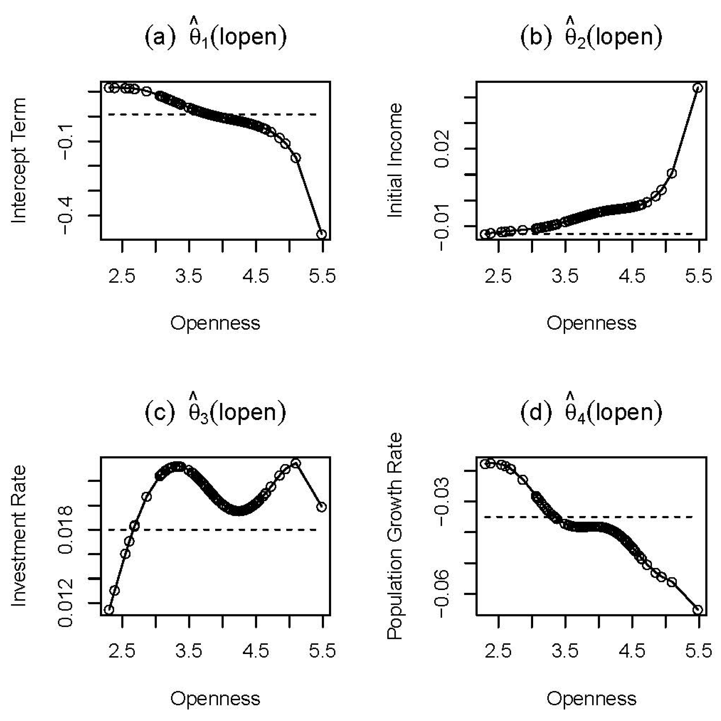The coefficient estimates, ${\tilde{\theta }}_1(·)$, ${\tilde{\theta }}_2(·)$, ${\tilde{\theta }}_3(·)$ and ${\tilde{\theta }}_4(·)$ are presented in Figure 1, where the solid lines with circles display the second-step estimates. The dashed lines represent the estimates of the spatially-augmented Solow growth model of [4] using the inverse power spatial weight function, which we include as a baseline. We interpret Figure 1 as follows. First, in Figure 1b, we see that there is a negative relation between the initial level of income and the economic growth rate, except for Mauritius, Hong Kong, Zambia, Cameroon and Singapore, which confirms a conditional β-convergence hypothesis. Moreover, we observe that ${\tilde{\theta }}_2(·)$ is increasing in openness, which, however, results in a gradually declining degree of convergence. In addition, we see that the nonparametric model reveals slightly weaker conditional economic growth convergence as compared to the parametric model.

Figure 1. Estimated coefficient curves.

Figure 1. Estimated coefficient curves.

Second, in Figure 1c, we see that ${\tilde{\theta }}_3(·)$ exhibits a positive, but not a monotonic, relation between the real investment rate and the real GDP per capita growth rate. Our estimate of the coefficient of the investment rate fluctuates as the trade openness of countries increases. For the economies with a trade openness higher than 15% of GDP, our result indicates that the nonparametric model sees stronger positive impact of the investment rate on the real GDP per capita growth rate than the parametric model does. Third, in Figure 1d, it is observed that the population growth rate has a negative impact on the real GDP per capita growth rate. For the countries whose trade openness ranges between 29% and 65%, our estimates for the coefficient of the population growth rate are relatively flat. Moreover, we note that the magnitude of the negative effect of the population growth rate is getting larger as the trade openness of countries increases, especially when the trade openness is over 65% of GDP. Overall, Figure 1 can be interpreted as the fact that an open economy suffers from higher negative impact of the population growth rate, but at the same time takes the advantage of high initial real GDP per capita.

Next, due to the cross-country interactions through spatial weights, the functional coefficient estimates have a different interpretation than the one obtained from the non-spatial model. In order to correctly interpret these estimates, we rewrite the estimated model in a reduced from as follows:

$$\begin{array}{ccc}\hfill Y& =& {(I_n-{\widehat{G}}_n)}^{-1}[{\widehat{M}}_{n}ln\left(y60\right)+{\tilde{\theta }}_1\left(lopen\right)+{\tilde{\theta }}_2\left(lopen\right)\odot ln\left(y60\right)\hfill \\ & & +{\tilde{\theta }}_3\left(lopen\right)\odot ln\left(s\right)+{\tilde{\theta }}_4\left(lopen\right)\odot ln(n+0.05)+\tilde{U}],\hfill \end{array}$$

(20)

where $\tilde{U}$ is the $n\times 1$ vector of residuals. Then, from Equation (20), the marginal effects are given by the following $n\times n$ matrices:

$$\begin{array}{cc}\hfill \frac{\partial E\left(Y\right|y60,s,n)}{\partial ln\left(y{60}^T\right)}& \equiv {(I_n-G_n)}^{-1}[M_n+diag\left\{{\theta }_2\left(lopen\right)\right\}]\hfill \\ \hfill \frac{\partial E\left(Y\right|y60,s,n)}{\partial ln\left(s^T\right)}& \equiv {(I_n-G_n)}^{-1}diag\left\{{\theta }_3\left(lopen\right)\right\}\hfill \\ \hfill \frac{\partial E\left(Y\right|y60,s,n)}{\partial ln(n^T+0.05)}& \equiv {(I_n-G_n)}^{-1}diag\left\{{\theta }_4\left(lopen\right)\right\}\hfill \end{array}$$

where we define $diag\left\{a\right\}$ as an $n\times n$ diagonal matrix with the elements of an $n\times 1$ vector, a, on the main diagonal. Following LeSage and Pace [10], we label the diagonal elements of each matrix given above as the direct impacts and off-diagonal elements as the indirect impacts.

In Table 2, we report the estimated average direct impact (ADI) and average indirect impact (AII) of the explanatory variables, where the latter can be easily defined as the difference between average total impact 4 and the average direct impact. Average direct and indirect impacts from the parametric model of [4] are denoted as ADI${}_{EK}$ and AII${}_{EK}$, respectively. The interpretation of Table 2 is as follows. Firstly, we observe that a 1% increase in the real initial GDP per capita of an economy, holding other factors fixed, results in a decrease by 0.5% in its own real GDP per capita growth rate. However, this change increases the rest of the economies’ economic growth rates by 0.01% on average due to the spatial dependence. From another point of view, a 1% increase in all of the regions’/nations’ initial real GDP per capita speeds up this economy’s real GDP per capita growth by 0.01%. This result indicates a positive spillover effect of the initial level of income. Secondly, a 1% increase in this economy’s real investment rate increases its own real GDP growth rate by 2.08% on average. However, this change slows down the rest of the nations’ real GDP growth by 0.08% on average. Thirdly, we see that a 1% increase in the population growth rate of this economy retards its own economic growth by 3.8% on average, but helps to improve the rate of economic growth of the rest of the countries by 0.16% on average.

Fourthly, when comparing our results to [4]’s results, we find that both the nonparametric and the parametric model give almost the same average direct effects of the initial per capita income, investment rate and population growth rate on the economic growth rate and that both models result in the same signs in the average direct and indirect effects. However, the AII values from the nonparametric model are much smaller than the results from the parametric model in absolute value, especially for the initial per capita income and the population growth rate. This is not surprising, as the parametric model assumes that all of the spatial weights take non-negative values, while our nonparametric spatial weights are estimated from the data without such a restriction. Although it is popular practice to assume non-negative spatial weights, this is an assumption imposed without support from econometric or economic theory. For example, trade treaties and monetary policies are both double-edged swords that may bring opposite impacts to different national economies, and non-negative spatial weights may not be able to capture the opposite interactions among different economies. As both [4]’s parametric SDM and our proposed semiparametric SDM approximate the unknown true relationships in their own best capacity, however, our model imposes less restrictions than the parametric SDM and is believed to bring a better fit to the data and more reliable inference. Although the numbers are different, both models give the same sign in estimated direct and indirect effects. Overall, we observe that the average direct and indirect effects can take opposite signs, and the effect of the former is much stronger than that of the latter in absolute magnitude.

Table 2. Average direct and indirect impact estimates.

	ln(y60)	ln(s)	ln(n + 0.05)
ADI	−0.0050	0.0208	−0.0381
	(−0.0122, −0.0005)	(0.0089, 0.0341)	(−0.0782, −0.0054)
ADI${}_{EK}$	−0.0119	0.0184	−0.0336
	(−0.0159, −0.0078)	(0.0139, 0.0229)	(−0.0585, −0.0094)
AII	0.0001	−0.0008	0.0016
	(−0.0077, 0.0056)	(−0.0174, 0.0190)	(−0.0347, 0.0289)
AII${}_{EK}$	0.0140	−0.0018	0.0275
	(0.0052, 0.0244)	(−0.0169, 0.0124)	(−0.0321, 0.0860)

Note: A 95% bootstrap percentile confidence interval is given in the parenthesis.

Table 2. Average direct and indirect impact estimates.

	ln(y60)	ln(s)	ln(n + 0.05)
ADI	−0.0050	0.0208	−0.0381
	(−0.0122, −0.0005)	(0.0089, 0.0341)	(−0.0782, −0.0054)
ADI${}_{EK}$	−0.0119	0.0184	−0.0336
	(−0.0159, −0.0078)	(0.0139, 0.0229)	(−0.0585, −0.0094)
AII	0.0001	−0.0008	0.0016
	(−0.0077, 0.0056)	(−0.0174, 0.0190)	(−0.0347, 0.0289)
AII${}_{EK}$	0.0140	−0.0018	0.0275
	(0.0052, 0.0244)	(−0.0169, 0.0124)	(−0.0321, 0.0860)

Note: A 95% bootstrap percentile confidence interval is given in the parenthesis.

LeSage and Pace [10] (p. 39) explain how to obtain the standard errors for the ADI and AII estimates via a simulation method. In the parametric setup, as the spatial weight matrices are known, theoretically, one can apply the delta method to obtain the standard errors, and the simulation method tends to provide at best an approximation as one does not know the exact distribution of the estimated coefficients in finite samples; however, this method is feasible as the average direct and indirect impacts only depend on a finite number of unknown parameters. As our proposed semiparametric model contains both unknown spatial weights and unknown coefficient curves, the simulation method would involve simulating from a joint distribution with dimension equal to $2n\left(n-1\right)$ (two spatial weight matrix estimates) plus $4n$ (four coefficient curve estimates) or 16,744 in our empirical application. Therefore, the simulation method is infeasible for our empirical interest here. As both the ADI and AII are in the form of sample averages and it is well known that the bootstrap method can be used to estimate the sample average and its standard error well (e.g., [49]), we decide to report our bootstrap estimates of the confidence intervals for the ADI and AII.

Below, we explain a residual-based bootstrap method to test whether the ADI and AII are significantly different from zero at the 5% significance level. We use the nonparametric bootstrap percentile method to construct a 95% confidence interval. Following [50,51], we first estimate the functional coefficients using an oversmoothed bandwidth, which tends to zero at a slower speed than the optimal bandwidth. Then, we obtain estimated residuals. The rest of the bootstrap procedure is given below.

• Resample the estimated residuals and obtain the bootstrap errors, $U^b$.
• Calculate:

  $$\begin{array}{c}{Y}^b={(I_n-{\widehat{G}}_n)}^{-1}[{\widehat{M}}_{n}ln\left(y60\right)+{\tilde{\theta }}_1^{*}\left(lopen\right)+{\tilde{\theta }}_2^{*}\left(lopen\right)\odot ln\left(y60\right)+\hfill \\ \hfill {\tilde{\theta }}_3^{*}\left(lopen\right)\odot ln\left(s\right)+{\tilde{\theta }}_4^{*}\left(lopen\right)\odot ln(n+0.05)+U^b],\end{array}$$

  where ${\tilde{\theta }}_k^{*}(·)$, $k=1,2,3,4$ are coefficient estimates using a larger bandwidth than the optimal bandwidth. Call ${\left\{ln\left(y{60}_i\right),ln\left(s_i\right),ln(n_i+0.05),Y^b\right\}}_{i=1}^n$ the bootstrap sample.
• Estimate Model (19) from the bootstrap sample, and record ${\tilde{\theta }}_1^b(·)$, ${\tilde{\theta }}_2^b(·)$, ${\tilde{\theta }}_3^b(·)$ and ${\tilde{\theta }}_4^b(·)$, the bootstrap estimates of the functional coefficients.
• Calculate the bootstrap value of average direct and indirect impacts of the explanatory variables, $AD{I}^b$ and $AI{I}^b$, respectively.
• Repeat Steps 1–4 for 999 times.
• Find the 0.025th and 0.975th empirical percentile of the 999 bootstrap values of ADI and AII and the point estimates given in Table 2 to establish the 95% bootstrap percentile confidence interval.

The confidence intervals are reported in Table 2. We see that the ADI values are statistically significantly different from zero at the 5% significance level. Moreover, we find that there is no significant effect on average from neighbouring countries per capita initial income, savings rate and population growth rate on economic growth rate of the country of interest. The same inference is obtained for the parametric model, except that the parametric model sees a significant average indirect impact of initial per capita income. Note that insignificant AIIs do not imply that the indirect impact from economy i on economy j is insignificant for all $\left(i,j\right)$.

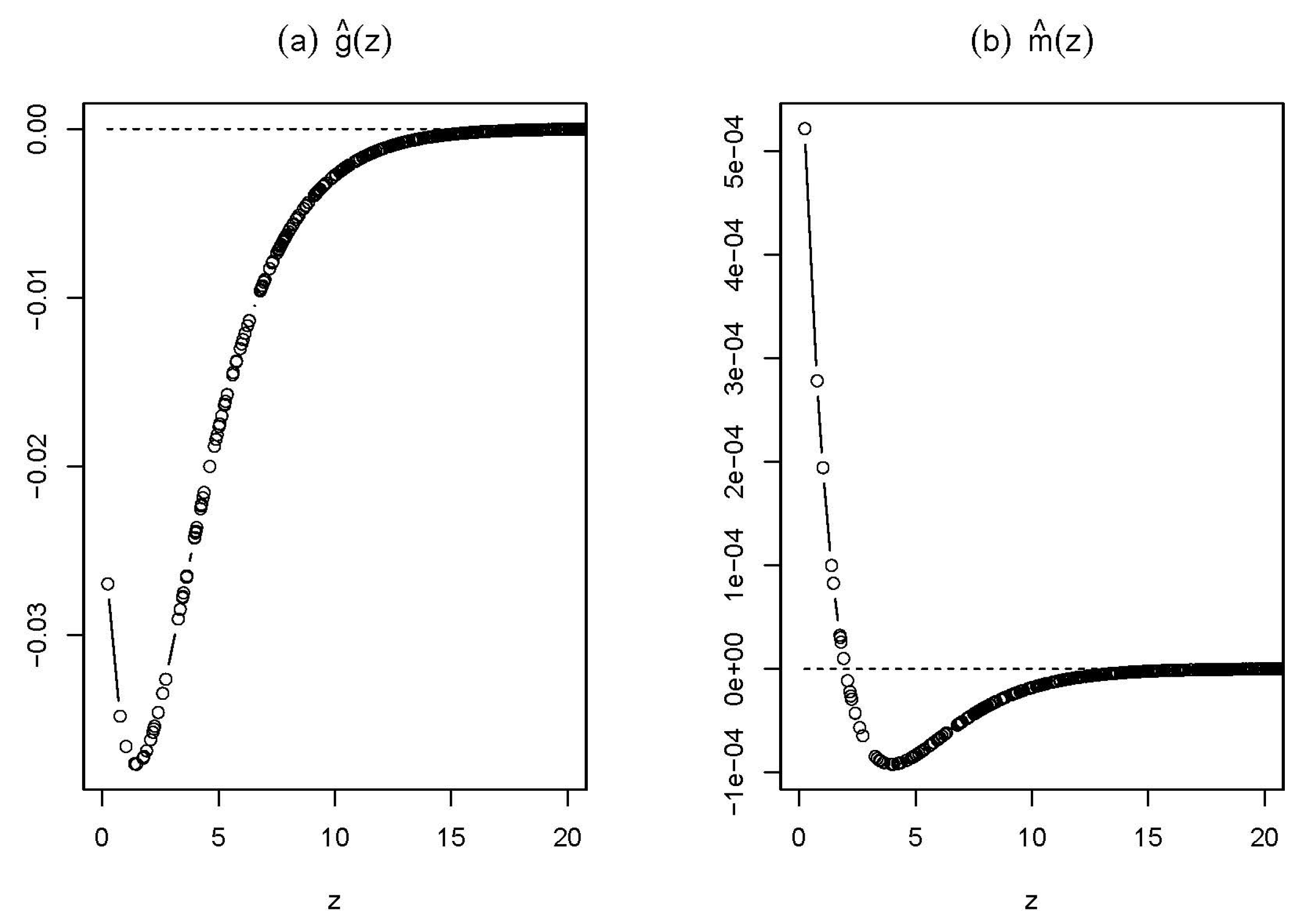
Figure 2 presents estimated spatial weighting functions. We plot both estimated spatial weighting functions, $\widehat{g}\left(·\right)$ and $\widehat{m}\left(·\right)$, for the geographic distances ranging from zero to 20 in 100 km, as the estimated spatial weights in the absolute value have an average of 5.069 × 10${}^{-7}$ and 3.893 × 10${}^{-9}$, respectively, when $z>20$. In Figure 2a,b, firstly, we see negative spatial weights, which greatly contradicts traditional parametric spatial regression models, which often assume non-negative spatial weights. Negative spatial interactions are indeed common in practice, especially in social networks; see [52,53] for strategic interactions within the monetary policy committee of the Bank of England. Secondly, both spatial weight functions are not strictly monotonic and exhibit convexity among nations that are not very far apart, concavity among nations with moderately far distances and a zero spatial weight function among nations that are far away. Moreover, the spatial weight functions take bigger absolute values among nations with smaller distance apart and smaller absolute values among far-away nations, which implies a relatively larger economic interaction among nearby nations than among far-away nations. Lastly, in Figure 2b, we observe positive estimated spatial weights when the distance ranges between 0.229 and 1.894, which correspond to 22.9 and 189.4 km, respectively. For the distances greater than 189.4 km, negative spatial weights are getting closer to zero as the distance between two countries increases. As the turning point 1.894 is really small and occurs for countries with a small area, our results imply that spatial interaction is very strong and different between two nearby small countries with small areas than between two countries with longer distances when at least one country has a large area.

Figure 2. Estimated spatial weighting functions.

Figure 2. Estimated spatial weighting functions.

6. Conclusions

We employ a spatial Durbin model combined with the nonparametric spatial weighting functions, as well as the unknown functional coefficients to estimate the augmented Solow growth model with a sample of 91 countries over the period 1960 to 1995. We find a negative spatial lag effect of neighbouring country’s GDP per capita growth rate and initial GDP per capita on the economic growth rate of country i. These effects are declining in magnitude as the geographical distance between the two countries increases. Finally, allowing coefficients as a function of trade openness of a country enables us to see the true country-specific effect of each determinant of economic growth. Moreover, we find significant average direct impact from each production factors. However, our findings show that the average indirect impact of these variables is insignificant at the 5% significance level.