Measurement Errors Arising When Using Distances in Microeconometric Modelling and the Individuals’ Position Is Geo-Masked for Confidentiality

Abstract

In many microeconometric models we use distances. For instance, in modelling the individual behavior in labor economics or in health studies, the distance from a relevant point of interest (such as a hospital or a workplace) is often used as a predictor in a regression framework. However, in order to preserve confidentiality, spatial micro-data are often geo-masked, thus reducing their quality and dramatically distorting the inferential conclusions. In particular in this case, a measurement error is introduced in the independent variable which negatively affects the properties of the estimators. This paper studies these negative effects, discusses their consequences, and suggests possible interpretations and directions to data producers, end users, and practitioners.

1. Introduction

In many microeconometric studies we often use distances. For instance in labor, in schooling, or in health studies, the distance between each observed individual and a conspicuous point (e.g., a hospital or the workplace or a school) is often used as a predictor in a regression model. Furthermore, if our aim is to take into account the interacting effects between individuals using econometrics methods [1], we often build up weight matrices based on some inverse-distance function, using the two by two distances between individuals as the basis for the calculation. When analyzing granular micro spatial data (like e.g., household surveys), in order to preserve confidentiality the coordinates of each individual are often displaced according to some random method. For instance some recent DHS surveys coordinates are first collected in the field using GPS receivers with an accuracy of less than 15 m, but then, in order to ensure that respondent confidentiality is maintained, the observed points are geo-masked along a random distance and a random angle (see, e.g., [2]) using different maximum error distances in urban and rural areas (see [3,4,5] for details). A second method is the Gaussian geo-masking which consists in randomly reallocating the point in the neighborhood of the true location, with a probability described by a Gaussian bivariate density function centered on the true point. This paper’s contribution consists in analyzing the problems induced by geo-masking in econometric models as a problem of measurement error. In Section 2 we will consider the measurement error induced by geo-masking in case the distance is used as a predictor in a regression model. Section 3 concludes with some practical comments and directions to assist the statistics producers to calibrate the geo-masking procedures before delivering the data to the public.

2. Effects of Geo-Masking When We Use the Distance as a Predictor in a Regression

2.1. Generalities

Let us consider the case of the estimation of a linear regression when the true individuals’ coordinates are not disclosed for confidentiality and a distance from a relevant point is used as a predictor. For instance, in health economics it is common practice to postulate a relationship between a health outcome for each individual (such as the effect of a health policy), say y, and the individual’s distance (say d) from a clinic or a hospital. To illustrate the essence of the problem we will restrict ourselves to the case, admittedly unrealistic, of a simple regression without any further predictors. Furthermore, to simplify the algebra without compromising the generality of the results, we will postulate a relationship between the health outcome and the squared distance from a relevant point. When data are geo-masked, the distance between each individual and a conspicuous point will be upward biased (as shown, e.g., by Arbia et al., 2015 [5] and Elkies, et al., 2015 [6]). This paper shows that, when the masking procedure is disclosed, this information can be taken into account for the benefit of the analysis.

To start with, let us recall that the classical error measurement theory (e.g., [7]) defines the true model as:

$$y_{ij}=\text{α}+\text{β}{d}_{ij}^2+v_{ij}$$

(1)

for each individual observed in the point of coordinates (i,j), with $d_{ij}$ the distance between point (i,j) and the point of interest and $v_{ij}\approx n.i.d.(0,{\sigma }_v^2)$. The distance is observed with an error due to geo-masking and the measurement error is defined as:

$$u_{ij}={\overline{d}}_{ij}^2-d_{ij}^2$$

with ${\overline{d}}_{ij}^2$ the squared distance observed after geo-masking. Following the classical theory, as it is known, u_ij should be assumed to be such that: $E(u_{ij})=0$, $Var(u_{ij})={\sigma }_u^2=$ constant, and u_ij independent of v_ij and of $d_{ij}^2$. Normality of u is also often assumed. In these conditions, having called $\widehat{\text{β}}$ the OLS estimator of β, such estimator will be still unbiased, but less efficient, since its variance can now be expressed as:

$$Var(\widehat{\text{β}})=\frac{{\text{β}}^2{\sigma }_u^2+{\sigma }_v^2}{n{\sigma }_{d^2}^2}>\frac{{\sigma }_v^2}{n{\sigma }_{d^2}^2}$$

(2)

The estimator will also be inconsistent with a downward asymptotic bias towards zero (called attenuation) quantified by the expression [7]:

$$p\lim \widehat{\text{β}}=\text{β}\left(\frac{{\sigma }_{d^2}^2}{{\sigma }_u^2+{\sigma }_{d^2}^2}\right)<\text{β}$$

(3)

with ${\sigma }_{d^2}^2$ the variance of the squared uncontaminated distances.

However, in the case of a measurement error induced by geo-masking, the results are quite different from the classical, as we will illustrate in the next sections.

2.2. Gaussian Geo-Masking within a Circle

Let us start considering the effect of geo-masking when using a distance as a regressor in an econometric model, in the case of Gaussian geo-masking, that is when the true individuals’ location is perturbated with a bivariate Gaussian distribution centered on the true point. More formally let us consider the point of coordinates (i,j) and let us geo-mask this point by disclosing, instead, the coordinates $\overline{i}=i+{\text{ε}}_i$ and $\overline{j}=j+{\text{ε}}_j$ with ${\text{ε}}_i\approx n.i.d.(0,{\sigma }_{\text{ε}}^2)$. Let us further consider, for each individual point, its distance from a conspicuous point that, without loss of generalities, we can allocate at the origin of the Cartesian system. In this case the true squared distance of the point of coordinates (i,j) from the conspicuous point is given by:

$$d_{ij}^2=i^2+j^2$$

while, after geo-masking we observe instead

$${\overline{d}}_{ij}^2={\overline{i}}^2+{\overline{j}}^2=d_{ij}^2+({\text{ε}}_i^2+{\text{ε}}_j^2)+2(i{\text{ε}}_i+j{\text{ε}}_j)=d_{ij}^2+u_{ij}$$

(4)

because of our definitions.

So the term u defines the measurement error on the independent variable of the model as in the classical theory. However, in contrast with the classical theory, in this case we have:

$$E(u_{ij})=2{\sigma }_{\text{ε}}^2\ne 0\forall i,j$$

(5)

and

$$Var(u_{ij})=4{\sigma }_{\text{ε}}^2\left({\sigma }_{\text{ε}}^2+d_{ij}^2\right)$$

(6)

Thus the measurement error has non-zero mean and non-constant variances. (See Appendix A for the proof). The non-zero mean does not affect the point estimate of the parameter β, but only the constant term. Equation (6) shows that the procedure of geo-masking also induces heteroscedasticity.

Furthermore from Equation (4) we have:

$$u_{ij}={\overline{d}}_{ij}^2-d_{ij}^2={\left(i+{\text{ε}}_i\right)}^2+{\left(j+{\text{ε}}_j\right)}^2-d_{ij}^2$$

(7)

As a consequence (since $d_{ij}^2$, i and j are constant terms and ${\text{ε}}_i\approx n.i.d.(0,{\sigma }_{\text{ε}}^2)$) $u\approx {\chi }_2^2(\lambda )$ is a non-central Chi-squared with 2 degrees of freedom and non-centrality parameter $\lambda =\frac{d_{ij}^2}{{\sigma }_{\text{ε}}^2}$. The proof is left to Appendix B.

Following the classical theory, the OLS estimator will be less efficient and inconsistent recalling Equations (2) and (3). In particular, in the case of Gaussian geo-masking, the variance of the OLS estimator will be:

$$Var{(\widehat{\text{β}})}_{ij}=\frac{4{\text{β}}^2{\sigma }_{\text{ε}}^2\left({\sigma }_{\text{ε}}^2+d_{ij}^2\right)+{\sigma }_v^2}{n{\sigma }_{d^2}^2}>\frac{{\sigma }_v^2}{n{\sigma }_{d^2}^2}$$

(8)

Thus, the larger are ${\sigma }_{\text{ε}}^2$ and the larger the distance from the conspicuous point is, the lower the precision of the estimate will be. The precision also depends on the square of the true value of β. Furthermore, using Equation (6) to evaluate the attenuation, we have:

$$p\lim \widehat{\text{β}}=\text{β}\left(\frac{{\sigma }_{d^2}^2}{{\sigma }_u^2+{\sigma }_{d^2}^2}\right)=\text{β}\left(\frac{{\sigma }_{d^2}^2}{4{\sigma }_{\text{ε}}^2\left({\sigma }_{\text{ε}}^2+d_{ij}^2\right)+{\sigma }_{d^2}^2}\right)$$

(9)

which shows that the attenuation effect on the OLS estimator is greater in the presence of a larger geo-masking variance of higher distances.

In practical cases, to communicate with practitioners, it is useful to introduce the Gaussian geo-masking mechanism with reference to a maximum displacement distance which is easier to interpret than a variance for non-specialists. Since in a Gaussian distribution $P(-3\sigma \le x\le 3\sigma )=0.9973$, with a probability close to 1 we can assume that the maximum displacement distance is 3σ. If we call θ* such maximum distance, we have that 3σ = θ*. So the expected measurement error is $E(u)=2{\sigma }_{\text{ε}}^2=\frac{2}{9}{\text{θ}}^{*2}$ and the bias can be seen as a fraction of the maximum squared displacement distance. Furthermore its variance can be expressed as $Var(u)=\frac{4}{81}{\text{θ}}^{*4}+\frac{8}{9}{\text{θ}}^{*2}{d}_{ij}^2$ which shows that uncertainty increases with the maximum displacement distance and with the absolute position of the individual with respect to the conspicuous point. By using this alternative expression, the variance of the OLS estimator can be expressed as:

$$Var{(\widehat{\text{β}})}_{ij}=\frac{{\text{β}}^2\left(\frac{4}{81}{\text{θ}}^{*4}+\frac{4}{9}{\text{θ}}^{*2}{d}_{ij}^2\right)+{\sigma }_v^2}{n{\sigma }_{d^2}^2}$$

(10)

and the attenuation effect as:

$$p\lim \widehat{\text{β}}=\text{β}\left(\frac{{\sigma }_{d^2}^2}{{\sigma }_u^2+{\sigma }_{d^2}^2}\right)=\text{β}\left(\frac{{\sigma }_{d^2}^2}{\frac{4}{81}{\text{θ}}^{*4}+\frac{4}{9}{\text{θ}}^{*2}{d}_{ij}^2+{\sigma }_{d^2}^2}\right)$$

(11)

which shows more intuitively the negative effects of geo-masking on the OLS estimates. The greater the maximum displacement distance is, the larger both the loss in efficiency and the attenuation effect will be.

2.3. Uniform Geo-Masking within a Circle

Let us now turn to analyze the effects of a uniform geo-masking (such as the one employed, e.g., by DHS, 2013 [4]), that is a mechanism which transforms the coordinates displacing them along a random angle (say δ) and a random distance (say θ) both obeying a uniform probability law. The mechanism can be formally expressed through the following hypotheses:

HP1:

$\text{θ}\stackrel{iid}{{\displaystyle \approx }}U(0,{\text{θ}}^{*})$ and $\delta \stackrel{iid}{{\displaystyle \approx }}U(0,360°)$, with θ* the maximum distance error, and

HP2:

θ and δ are independent.

Assuming again, without loss of generality, that the conspicuous point is located in the origin, the true squared distance between point of coordinates (i,j) and the conspicuous point before geo-masking is measured by $d_{ij}^2=(i^2+j^2)$, while, after geo-masking, it can be expressed, using the polar coordinates, as:

$${\overline{d}}_{ij}^2={(i+\text{θ}Cos\delta )}^2+{(j+\text{θ}Sin\delta )}^2$$

(12)

Expanding Equation (12) we obtain:

$${\overline{d}}_{ij}^2=(i^2+2i\text{θ}Cos\delta +{\text{θ}}^{2}Co{s}^2\delta +j^2+2j\text{θ}Sin\delta +{\text{θ}}^{2}Si{n}^2\delta )$$

so that we can now express the measurement error as:

$$u_{ij}={\overline{d}}_{ij}^2-d_{ij}^2=2\text{θ}\left(iCos\delta +jSin\delta \right)+{\text{θ}}^2\left(Co{s}^2\delta +Si{n}^2\delta \right)$$

(13)

Similarly to the Gaussian case we have a non-zero mean and a non-constant variance, given by:

$$E(u_{ij})=\frac{{\theta }^{*}}{3}\ne 0$$

(14)

and

$$Var(u_{ij})=\frac{17}{180}{\text{θ}}^{*4}+\frac{2}{3}{\text{θ}}^{*2}{d}_{ij}^2$$

(15)

Again the proofs are left to the appendices, specifically to Appendix C.

So, consistently with the results obtained with a Gaussian geo-masking and according with the intuition, the measurement error increases its variance as the maximum displacement distance θ* increases and as we move away from the conspicuous point.

If we use this result again to provide an explicit expression to the estimation variance and to the attenuation effect, we have, respectively:

$$Var{(\widehat{\text{β}})}_{ij}=\frac{{\text{β}}^2\left(\frac{17}{180}{\text{θ}}^{*4}+\frac{2}{3}{\text{θ}}^{*2}{d}_{ij}^2\right)+{\sigma }_v^2}{n{\sigma }_{d^2}^2}$$

(16)

and

$$p\lim \widehat{\text{β}}=\text{β}\left(\frac{{\sigma }_{d^2}^2}{{\sigma }_u^2+{\sigma }_{d^2}^2}\right)=\text{β}\left(\frac{{\sigma }_{d^2}^2}{\frac{17}{180}{\text{θ}}^{*4}+\frac{2}{3}{\text{θ}}^{*2}{d}_{ij}^2+{\sigma }_{d^2}^2}\right)$$

(17)

which lead to very similar conclusions to those found for the Gaussian geo-masking (see Equations (10) and (11)). The greater the maximum displacement distance is, the lower the precision and the larger the attenuation effects are.

3. Discussion and Conclusions

In this paper we examined the measurement error on distances introduced by the procedure of geo-masking the individuals’ true location to protect their confidentiality, when such distances are used as predictors in a linear regression. The formal expressions that we derived for the loss in efficiency and for the attenuation in the case of Gaussian and uniform geo-masking, are very important under the practical point of view. In fact, the true location of each of the observed individuals is known to the producer of the official statistics before the displacement is introduced and so it is the variance term ${\sigma }_{d^2}^2$. So, in principle, the data producers could calculate the appropriate expression before geo-masking the data when choosing the maximum location error (θ*) so as to limit the negative consequences on the subsequent analysis. Furthermore, the data producer could disclose to the end users and to the practitioners the level of attenuation which is expected given the chosen geo-masking procedure. In fact, for any given dataset, Expressions (11) and (17) are just functions of the maximum displacement distance θ*.

To illustrate this point, suppose, for instance, that n = 100 individuals have been observed in a unitary squared study area as it is shown in Figure 1.

Taking these points as given we have that $d_{ij}^2$ = 0.520151 (considering for operational reasons the mean of all squared distances from the origin) and ${\sigma }_{d^2}^2$ = 0.1592879. Figure 2 reports the behavior of the attenuation effect for Gaussian and uniform geo-masking for the values of the maximum displacement distance θ* ranging between 0 and 1.44 (1.44 being the theoretical maximum possible distance in a unitary square).

Two features emerge from the inspection of the graph. First, the attenuation increases dramatically already at small levels of θ*. Secondly, the Gaussian geo-masking, other things being constant, produces more severe consequences on the estimation of β than the uniform geo-masking. This graph could be used by the data producers to calibrate the optimal value of θ* and to communicate to the practitioners the resulting level of attenuation they should expect from a regression analysis.

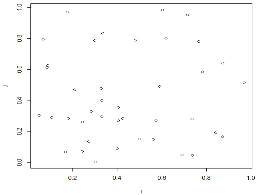
Figure 1. Spatial coordinates of n = 100 individuals located in a unitary square.

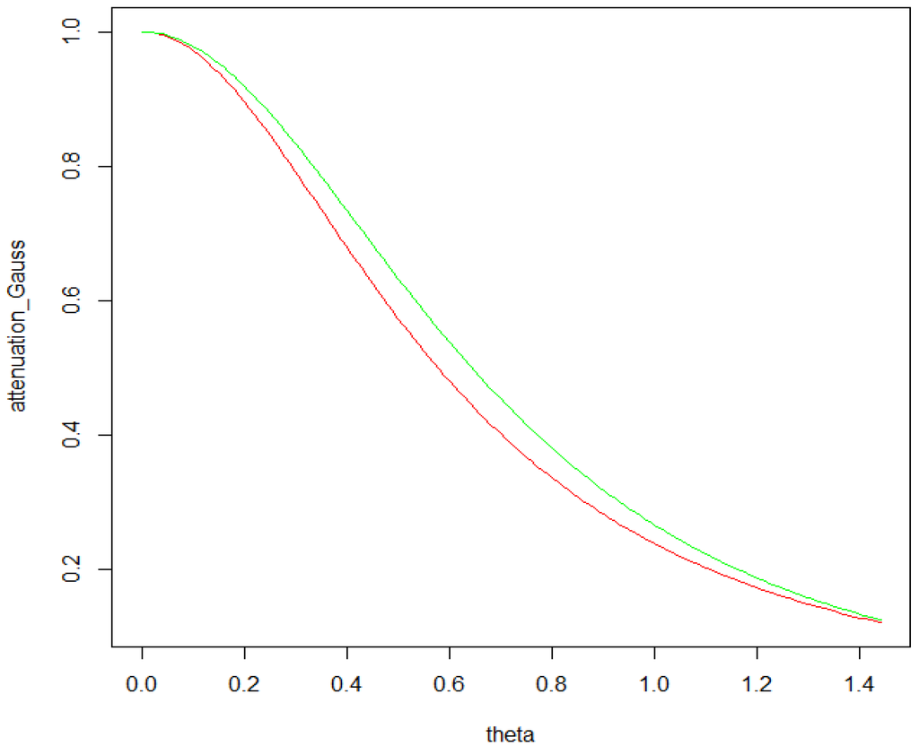
Figure 1. Spatial coordinates of n = 100 individuals located in a unitary square.

Figure 2. Attenuation effect in the presence of geo-masking as a function of the maximum displacement distance θ*. Gaussian geo-masking (red line). Uniform geo-masking (green line).

Figure 2. Attenuation effect in the presence of geo-masking as a function of the maximum displacement distance θ*. Gaussian geo-masking (red line). Uniform geo-masking (green line).

References

- G. Arbia. A Primer for Spatial Econometrics. London, UK: Palgrave Mac Millan, 2014. [Google Scholar]
- B. Collins. Boundary Respecting Point Displacement. Python Script; Arlington, VA, USA: Blue Raster, LLC, 2011. [Google Scholar]
- C.R. Burgert, J. Colston, T. Roy, and B. Zachary. “Geographic displacement procedure and georeferenced data release policy for the Demographic and Health Surveys.” In DHS Spatial Analysis Report No. 7. Calverton, MA, USA: ICF International, 2013. [Google Scholar]
- DHS. Spatial Analysis Report 8. Guidelines on the Use of GPS DHS Data. Calverton, MD, USA: ICF Interactional, September 2013. [Google Scholar]
- G. Arbia, G. Espa, and D. Giuliani. “Dirty spatial econometrics.” Ann. Reg. Sci., 2015. submitted. [Google Scholar]
- N. Elkies, G. Fink, and F.G. Baernighausen. “Scrambling geo-referenced data to protect privacy induces bias in distance estimation.” Popul. Environ. 37 (2015): 83–98. [Google Scholar] [CrossRef]
- M. Verbeek. A guide to Modern Econometrics. Chichester, UK: Wiley, 2004. [Google Scholar]
© 2015 by the authors; licensee MDPI, Basel, Switzerland. This article is an open access article distributed under the terms and conditions of the Creative Commons Attribution license ( http://creativecommons.org/licenses/by/4.0/).