Article

Binance USD Delisting and Stablecoins Repercussions: A Local Projections Approach

by
Papa Ousseynou Diop
and
Julien Chevallier
*
Economics Department, Université Paris 8 (LED), 2 Rue de la Liberté, 93526 Saint-Denis, France
*
Author to whom correspondence should be addressed.
Econometrics 2026, 14(1), 6; https://doi.org/10.3390/econometrics14010006
Submission received: 31 October 2025 / Revised: 8 January 2026 / Accepted: 12 January 2026 / Published: 16 January 2026

Abstract

The delisting of Binance USD (BUSD) constitutes a major regulatory intervention in the stablecoin market and provides a unique opportunity to examine how targeted regulation affects liquidity allocation, market concentration, and short-run systemic risk in crypto-asset markets. Using daily data for 2023 and a linear and nonlinear Local Projections event-study framework, this paper analyzes the dynamic market responses to the BUSD delisting across major stablecoins and cryptocurrencies. The results show that liquidity displaced from BUSD is reallocated primarily toward USDT and USDC, leading to a measurable increase in stablecoin market concentration, while decentralized and algorithmic stablecoins absorb only a limited share of the shock. At the same time, Bitcoin and Ethereum experience temporary liquidity contractions followed by a relatively rapid recovery, suggesting conditional resilience of core crypto-assets. Overall, the findings document how a regulatory-induced exit of a major stablecoin reshapes short-run market dynamics and concentration patterns, highlighting potential trade-offs between regulatory enforcement and market structure. The paper contributes to the literature by providing the first empirical analysis of the BUSD delisting and by illustrating the usefulness of Local Projections for studying regulatory shocks in cryptocurrency markets.

1. Introduction

The delisting of Binance USD (BUSD), a leading USD-pegged stablecoin Cole (2024), represents a significant milestone in the advancement of cryptocurrency regulation and highlights the increasing scrutiny that U.S. regulatory authorities are directing toward stablecoin issuers Lunde (2023). BUSD, issued by Paxos Trust Company and branded by Binance, recognized as the largest cryptocurrency exchange globally by trading volume Wilmarth (2023), exemplifies the intricate dynamics between conventional financial regulation and innovative digital assets Duan and Urquhart (2023).
The regulatory actions against BUSD have emerged within a broader framework of intensified oversight following the collapse of Terra/LUNA and FTX in 2022 Trautman et al. (2024). These incidents prompted heightened attentiveness from regulatory bodies concerning the operational frameworks of stablecoins and their associated systemic risks Goforth (2023). In February 2023, the New York Department of Financial Services (NYDFS) mandated that Paxos cease the minting of new BUSD tokens, citing unresolved issues regarding Paxos’s oversight of its relationship with Binance, as well as concerns related to Binance’s comprehensive compliance framework Zijing (2023).
This regulatory intervention signifies a fundamental shift in the stance of U.S. authorities concerning stablecoin governance, accentuating the critical necessity for robust compliance mechanisms and transparent operational structures Dell’Erba (2023). The actions taken against BUSD particularly underscore regulators’ growing apprehension regarding the potential use of stablecoins in facilitating illicit financial activities, which underscores the need for enhanced Anti-Money Laundering (AML) and Know Your Customer (KYC) protocols Skinner (2023).
Subsequent legal proceedings involving Changpeng Zhao (CZ), the CEO of Binance, further complicate the discourse surrounding BUSD’s delisting Qiǎn (2023). The criminal charges and the substantial settlement reached with U.S. authorities in late 2023 have raised fundamental questions pertaining to the intersection of centralized exchange operations and regulatory compliance Gushterov (2023). This development, in conjunction with the delisting of BUSD, represents a pivotal moment in the structural and governance framework of the cryptocurrency market Aujus (2023).
A critical inquiry arises regarding the broader implications of the delisting of BUSD for the stablecoin ecosystem: To what extent does this regulatory action alter the competitive dynamics among remaining stablecoin issuers, and what are the implications for market concentration within the stablecoin sector? Initial market data indicates a significant redistribution of liquidity toward alternative stablecoins, particularly Tether (USDT) and USD Coin (USDC). This consolidation prompts essential considerations regarding systemic risk and market power within the digital asset ecosystem Bains et al. (2022).
The growing prominence of stablecoins has reignited debates about their implications for financial stability and systemic risk. Systemic risk, broadly defined as the risk of disruptions in the financial system with severe consequences for the real economy Acharya et al. (2017), has increasingly been applied to the digital asset space. Recent research highlights the potential fragility of stablecoin arrangements and their spillover channels. For example, Giudici et al. (2022) analyze basket-based stablecoins and show how diversification mechanisms may mitigate, but also propagate, risks across tokens. R. Ahmed and Aldasoro (2025) further demonstrate that stablecoin dynamics can directly affect the pricing of traditional safe assets, underscoring their growing relevance for mainstream financial markets. More broadly, Aquilina et al. (2025) stress that cryptocurrencies and decentralized finance (DeFi) introduce novel functions that, while fostering innovation, also pose new challenges for financial stability.
Against this backdrop, our paper examines the repercussions of the BUSD delisting episode, focusing on its impact on the dynamics of competing stablecoins. By employing a local projections framework, we contribute to the literature on stablecoins’ systemic role, while providing empirical evidence on substitution and spillover effects that have direct policy relevance.
Furthermore, the case of BUSD’s delisting presents a compelling research question concerning the role of regulatory actions in shaping market structure: Does increased regulatory scrutiny of major market participants inevitably lead to greater concentration among a smaller number of compliant entities, thereby potentially engendering new forms of systemic risk? This paradox warrants thorough examination from both regulatory and economic perspectives.
The body of literature on stablecoins is expanding rapidly. Recent research by Łęt et al. (2023) explores the function of stablecoins as safe-haven assets amid cryptocurrency volatility. Utilizing spectral decomposition of variance for frequency-domain analysis, the study investigates the influence of shocks in assets such as Bitcoin and Ethereum on investor behavior in stablecoins. The analysis employs daily data from December 2017 to July 2022, encompassing significant stablecoins (e.g., Tether, USD Coin, Binance USD, DAI, Paxos, Huobi USD, and Gemini USD) alongside volatile cryptocurrencies (Bitcoin, Ethereum, Litecoin, and a composite index). The findings suggest that volatility shocks moderately affect stablecoin popularity over a period of up to three days, with negative returns and increased volatility prompting investors—especially smaller investors—to gravitate toward stablecoins, thereby highlighting their role in stabilizing markets during periods of financial uncertainty.
In a related investigation, Galati and Capalbo (2024) examined the ramifications of the collapse of Silicon Valley Bank in March 2023 on cryptocurrency markets, with a focus on stablecoins. By applying a BEKK-GARCH multivariate model to minute-by-minute price data for Bitcoin and five major stablecoins (USDT, BUSD, USDC, DAI, and TUSD) over a 14-day period surrounding the bankruptcy, their analysis reveals significant volatility spillovers. Notably, when Circle announced that $3.3 billion of USDC reserves were trapped in Silicon Valley Bank, marked market reactions occurred: USDC and DAI experienced substantial declines in price, and TUSD lost nearly 3% of its value, while BUSD and USDT traded at a premium. Increasing trading volumes further indicate a flight to safety towards more established stablecoins such as USDT.
With regard to the role of stablecoins as “anchors” within cryptocurrency markets, Palazzi et al. (2025) presents a comprehensive analysis of their stability, independence, and resilience. Employing asymmetric dynamic conditional correlation (ADCC)-GARCH models, Granger causality tests, and transfer entropy measures, the study evaluates data from major stablecoins (Tether, USD Coin, Binance USD), unpegged cryptocurrencies (Bitcoin, Ethereum, Binance Coin), and fiat currencies (EUR, JPY, GBP). The research uncovers significant vulnerabilities in stablecoin performance. Through methodical econometric analysis of liquidity conditions and market dynamics—particularly during adverse events such as the Terra-Luna collapse, as previously examined by Diop (2024), Diop et al. (2024) —these studies conclude that stablecoins’ susceptibility to market pressures and external shocks challenges their assumed role as stable monetary instruments, bearing critical implications for investors, policymakers, and regulators in the evolving cryptocurrency ecosystem.
Recent work has emphasized the importance of nonlinear and state-dependent dynamics in cryptocurrency markets. Dimitriadis et al. (2025), for instance, employ quantile-based and volatility models to study heterogeneous spillover effects across market conditions, showing that transmission mechanisms differ markedly between normal and stress periods. This focus on state dependence is closely related to our approach, which allows for asymmetric responses to regulatory shocks through linear and nonlinear Local Projections.
While Dimitriadis et al. (2025) analyze endogenous spillovers and volatility transmission across global cryptocurrency markets, our study focuses on the effects of a discrete regulatory intervention—the BUSD delisting—and its implications for liquidity reallocation and market structure within the stablecoin ecosystem. In this sense, the two approaches are complementary: their results highlight heterogeneity across market states, whereas our analysis documents how a targeted regulatory shock propagates through stablecoin and cryptocurrency markets over time.
Recent findings accentuate the increasing interdependence between traditional banking and cryptocurrency markets, providing critical insights for academics, practitioners, and policymakers who are concerned with systemic risk. While the study primarily addresses highly liquid digital assets, it establishes a foundation for further examination of financial contagion mechanisms that exist between conventional finance and digital assets.
To investigate the BUSD delisting, this paper employs the Local Projections approach, a method first introduced by Jordà (2005). Local projections represent an alternative technique for estimating impulse responses without the necessity of specifying and estimating a comprehensive multivariate dynamic system, such as a vector autoregression (VAR). Rather than depending on a global model, local projections derive impulse responses directly at each forecast horizon through a series of linear regressions, thereby enhancing robustness to model misspecification. This methodology permits more straightforward estimation through standard regression techniques, accommodates flexible nonlinear specifications, and facilitates analytical inference without the reliance on asymptotic approximations. Monte Carlo simulations and empirical applications validate the method’s advantages in accurately capturing impulse response dynamics, particularly within nonlinear and time-varying contexts.
Montiel Olea and Plagborg-Møller (2021) significantly contribute to the academic discourse surrounding local projections by confirming their robustness and simplicity for impulse response inference. The authors illustrate that lag-augmented local projections, when combined with standard heteroscedasticity-robust standard errors, produce valid asymptotic inference consistently across both stationary and non-stationary data processes. This reliability persists as horizons extend proportionally with sample size h T T η for η [ 0 , 1 ) . This is in contrast to traditional autoregressive approaches, whose validity heavily relies on the persistence characteristics and horizon lengths involved. By establishing that lag augmentation eliminates the necessity for serial correlation adjustments in standard errors, this paper simplifies applied analyses while addressing significant weaknesses inherent in vector autoregression methods related to unit roots and identification. These theoretical advancements effectively resolve longstanding concerns regarding the inferential validity of local projections, thereby reinforcing their reputation as a robust alternative within structural macroeconomics.
Bruns and Lütkepohl (2022) underscore the advantages of local projection (LP) estimators over conventional vector autoregression (VAR) models in structural macroeconomic analysis, particularly in proxy VAR frameworks. While impulse responses derived from VAR models depend on nonlinear transformations of estimated coefficients, LP estimators utilize direct linear regressions for each horizon, rendering them nonparametric and robust against model misspecification. This robustness is particularly significant when the actual data-generating process (DGP) diverges from a finite-order VAR structure, as LP estimators can mitigate biases stemming from incorrect lag specifications. The authors note that modified LP estimators—such as generalized least squares (GLSs) variants with lag augmentation—demonstrate enhanced small-sample performance, achieving lower root mean squared errors (RMSEs) compared to standard LP and VAR methods. For instance, a lag-augmented GLS estimator performs comparably to VAR estimators in larger samples, while maintaining computational simplicity and eliminating the necessity for extensive system estimation. Such features render LP methods particularly valuable for applied researchers who require reliable inference in environments characterized by model uncertainty.
The simulation study conducted by Li et al. (2024) provides essential insights into the bias-variance trade-offs between Local Projection (LP) and Vector Autoregression (VAR) methodologies for estimating structural impulse responses across numerous empirically calibrated macroeconomic data-generating processes (DGPs). The analysis indicates that LP estimators consistently display lower bias than VAR methodologies at both intermediate and long horizons, particularly when bias-correction techniques are employed. This characteristic is particularly valuable as LP methods avoid reliance on potentially misspecified VAR extrapolations. Utilizing DGPs constructed from a dynamic factor model fitted to 207 U.S. macroeconomic series, the authors replicate the complex persistence and cointegration patterns that are characteristic of real-world data. This strategy significantly enhances the external validity of their findings. Although LP methods may incur higher variance, particularly at extended horizons, their direct estimation approach is notably beneficial when researchers prioritize unbiased identification of impulse response shapes over precision. This consideration is especially pertinent in persistent macroeconomic systems, where restrictions on VAR lag length may induce substantial dynamic misrepresentation. Accordingly, these findings position LP as a highly compelling methodological alternative for structural macroeconometric analysis, warranting further investigation into bias correction and efficiency improvements in order to fully leverage its flexibility in capturing genuine economic dynamics.
Furthermore, the study employs nonlinear local projections organized under a regime-switching representation, utilizing a dummy variable to specify the threshold differentiation. M. I. Ahmed and Cassou (2016) operationalize this technique to analyze the state-dependent effects of consumer confidence shocks on durable goods spending. By incorporating NBER business cycle dates to create regime-switching dummies, they delineate asymmetric responses: confidence shocks substantially influence durable goods spending during expansive periods (consistent with news-driven expectations) but have negligible effects during recessive periods (which align with animal spirits theory). The nonlinear local projections model, augmented with a threshold dummy variable, establishes a flexible and robust framework for examining state-dependent economic dynamics. By accommodating regime-specific responses to shocks, this model adeptly captures the differential effects of the variables under investigation during various phases of the business cycle. This methodological approach may prove particularly advantageous in documenting the impact of BUSD delisting on other stablecoins, depending on the relevant regime.
In accordance with the Markov-switching approach, Gonçalves et al. (2024) advocate that a state-dependent approach to local projections (LPs) presents a valuable method for estimating the dynamic responses of macroeconomic variables to shocks, particularly in contexts characterized by nonlinearities across different economic states (e.g., recession versus expansion). This approach is advantageous due to its computational simplicity when compared to more complex models, such as state-dependent structural VARs, which necessitate detailed specifications for state transitions. State-dependent LP estimates facilitate the differentiation of impulse responses across varying economic states without the necessity to directly model state transition processes, thus rendering the methodology more flexible and user-friendly. However, the effectiveness of this approach is contingent upon whether the economic state is exogenous or endogenous to macroeconomic shocks. In scenarios where the state is exogenous, the method reliably estimates both conditional average and marginal responses to shocks. Conversely, if the state is endogenous, particularly in the presence of substantial shocks, the LP estimator may be biased. This underscores the critical importance of meticulously considering the magnitude of shocks and the nature of state dependence when employing this technique.
In a related nonlinear methodology for Local Projections, Auerbach and Gorodnichenko (2012) establish a framework for estimating state-dependent fiscal multipliers through the application of Smooth-Transition VAR (STVAR) and direct projection methods.
The delisting of Binance USD (BUSD) signifies a critical regulatory intervention with extensive implications for the stablecoin ecosystem. This study illustrates that the liquidity displaced from BUSD predominantly reallocates to centralized, fiat-backed stablecoins, specifically Tether (USDT) and USD Coin (USDC), thereby reinforcing their supremacy as systemic anchors. This swift redistribution highlights the market’s preference for liquidity depth and regulatory compliance; however, it simultaneously increases concentration risks, rendering the ecosystem susceptible to shocks affecting these limited entities. In contrast, algorithmic and decentralized stablecoins, such as DAI and FRAX, exhibit limited capacity to absorb this displaced liquidity, indicative of market skepticism regarding their stabilization mechanisms during periods of crisis. Their hybrid frameworks, whether crypto-collateralized or algorithmic, fail to instill confidence, underscoring the limitations inherent in non-fiat-backed designs with respect to accommodating systemic liquidity shocks.
Regarding traditional cryptocurrencies, the delisting induces asymmetric effects: Bitcoin (BTC) and Ethereum (ETH) encounter temporary liquidity contractions due to the disruption of trading pairs and decentralized finance (DeFi) activities resulting from stablecoin instability. Nevertheless, their long-term resilience underscores their dual role as speculative assets and essential liquidity reservoirs. Smaller cryptocurrencies, such as TRX, experience only momentary spikes in demand, failing to serve as sustainable alternatives. These dynamics illustrate the interconnectedness between stablecoins and the broader cryptocurrency market, wherein disruptions in stablecoins may induce short-term volatility without fundamentally destabilizing well-established assets such as BTC or ETH.
This research suggests a potential paradox: an increase in regulatory scrutiny directed at major players may lead to enhanced concentration among a smaller number of compliant entities, thereby potentially engendering new forms of systemic risk. These findings contribute to a deeper understanding of the intricate interplay between regulatory actions, market dynamics, and systemic risks within the evolving landscape of stablecoins and cryptocurrencies.
The remainder of the article is structured as follows. Section 2 details the linear and nonlinear Local Projection methods. Section 3 presents the BUSD and other associated stablecoins under study, both in prices and volumes. Section 4 contains the Local Projections results from the linear approach. Section 5 adds the regime-switching nonlinear version of Local Projections. Section 6 concludes.

2. Models

We detail first the “vanilla” model of Local projections, followed by enhancements under the form of nonlinear specifications with regime-switching.

2.1. Local Projections for Impulse Responses

The local projection method, as introduced by Jordà (2005), presents a flexible and robust strategy for estimating impulse responses without necessitating the specification of an underlying multivariate dynamic system. This methodology is characterized by the estimation of a sequence of regressions corresponding to each horizon of interest, rather than relying on a single global model such as vector autoregression (VAR). This approach is particularly advantageous in scenarios where the true data-generating process (DGP) remains unknown or is mispecified.

2.1.1. Impulse Response Definition

Let y t denote an n × 1 vector of endogenous variables at time t. The impulse response at horizon s is formally defined as the difference between two conditional expectations.
I R ( t , s , d i ) = E ( y t + s | y t = d i ; X t ) E ( y t + s | y t = ; X t ) , s = 0 , 1 , 2 ,
Here, E ( · | · ) represents the best mean squared error predictor, X t = ( y t 1 , y t 2 , ) denotes the history of the process up to time t 1 , d i is an n × 1 vector representing the experimental shock to the i-th variable, and ∅ is an n × 1 vector of zeros representing the absence of a shock. The impulse response I R ( t , s , d i ) captures the dynamic effect of the shock d i on the vector y t + s at horizon s.

2.1.2. Local Projection Regression

To estimate the impulse response, Jordà (2005) proposes projecting y t + s onto the linear space generated by the lags of y t . Specifically, for each horizon s, the following regression is estimated:
y t + s = α s + B 1 s + 1 y t 1 + B 2 s + 1 y t 2 + + B p s + 1 y t p + u t + s s , s = 0 , 1 , 2 , , h
In this equation, α s is an n × 1 vector of constants, B j s + 1 are n × n matrices of coefficients for each lag j and horizon s + 1 , and u t + s s is the error term at horizon s. The lag length p can be determined using information criteria such as the Akaike Information Criterion (AIC) or the Bayesian Information Criterion (BIC).
The impulse response at horizon s is then obtained from the estimated coefficients of the local projection regression:
I R ^ ( t , s , d i ) = B ^ 1 s d i , s = 0 , 1 , 2 , , h
where B ^ 1 s is the estimated coefficient matrix from the local projection regression. This approach directly estimates the impulse response coefficients, bypassing the need for iterative forecasting or inversion of a VAR model.

2.1.3. Inference and Robust Standard Errors

Inference for the impulse responses is straightforward with local projections, as the coefficients B ^ 1 s are estimated directly from the regression. To account for potential heteroskedasticity and autocorrelation in the error terms u t + s s , Jordà (2005) recommends using heteroskedasticity and autocorrelation consistent (HAC) robust standard errors. The variance–covariance matrix of the coefficients B ^ 1 s is denoted by Σ s , and a 95% confidence interval for the impulse response at horizon s is constructed as:
I R ^ ( t , s , d i ) ± 1.96 d i Σ s d i
This confidence interval serves as an important measure of the uncertainty associated with the estimated impulse responses, enabling valid inferences even when faced with model misspecification or nonlinearities in the data generating process (DGP).

2.1.4. Advantages over VAR-Based Methods

The local projection method offers several notable advantages compared to traditional VAR-based approaches. Firstly, it does not necessitate the specification of a global model, thereby enhancing its robustness against potential misspecifications in the DGP. Secondly, this method accommodates nonlinearities and flexible functional forms by permitting the inclusion of higher-order polynomial terms or threshold effects within the local projection regressions. Thirdly, inference is streamlined, as the impulse response coefficients can be estimated directly, removing the need for delta-method approximations or simulation-based techniques.

2.2. Nonlinear Local Projections with Regime-Switching: A Threshold Dummy Variable Approach

In recent years, the examination of nonlinear dynamics in macroeconomic models has attracted significant scholarly attention, particularly in the context of regime-switching models. The framework proposed by M. I. Ahmed and Cassou (2016) introduces a nonlinear local projections approach that integrates a threshold dummy variable to differentiate between distinct economic states, such as expansions and recessions. This methodology allows for the estimation of state-dependent impulse response functions (IRFs) and variance decompositions, thereby providing valuable insights into how economic shocks propagate differently across various regimes. This section offers a comprehensive exposition of the model, emphasizing the regime-switching specification alongside the threshold dummy variable.
The model developed by M. I. Ahmed and Cassou (2016) extends the foundational local projections framework established by Jordà (2005) by incorporating regime-switching behavior. A key innovation of this approach is the introduction of a threshold dummy variable to distinguish between varying economic states, as defined by the National Bureau of Economic Research (NBER) business cycle index. The model is articulated as follows:

2.2.1. Baseline Specification

The baseline linear local projections model is given by:
x t + s = α s + i = 1 p B i s + 1 x t i + u t + s s , s = 0 , 1 , , h ,
where x t = [ c t , c t , y t , f t ] is a vector of model variables, including consumer confidence ( c t ), consumption ( c t ), income ( y t ), and financial assets ( f t ). The term α s is a vector of constants, B i s + 1 represents the coefficient matrices for the i-th lag, and u t + s s is the error term. The model forecasts the variables s steps ahead using p lags of the variables in the system.

2.2.2. Threshold Local Projections

To incorporate regime-switching behavior, M. I. Ahmed and Cassou (2016) extend the linear model by introducing a threshold dummy variable I t , which takes the value 1 during recessions and 0 during expansions. The threshold model is specified as:
x t + s = I t 1 α R s + i = 1 p B i , R s + 1 x t i + ( 1 I t 1 ) α E s + i = 1 p B i , E s + 1 x t i + u t , t + s s ,
where α R s and α E s are regime-specific constants, and B i , R s + 1 and B i , E s + 1 are regime-specific coefficient matrices for the i-th lag. The error term u t , t + s s is also regime-specific. The threshold dummy variable I t is defined as:
I t = 1 if the economy is in a recession at time t , 0 if the economy is in an expansion at time t .

2.2.3. Impulse Response Functions

The impulse response functions (IRFs) for the threshold model are defined separately for each regime. For the recession regime, the IRF is given by:
I R ^ R ( t , s , d i ) = B ^ 1 , R s d i , s = 0 , 1 , , h ,
and for the expansion regime, the IRF is given by:
I R ^ E ( t , s , d i ) = B ^ 1 , E s d i , s = 0 , 1 , , h ,
where d i is a vector mapping the structural shock for the i-th element of x t to the experimental shocks. The IRFs are estimated using the local projection method, which allows for flexible estimation of the response functions without imposing the dynamic restrictions inherent in vector autoregression (VAR) models.

2.2.4. Variance Decomposition

The variance decomposition analysis is conducted to assess the contribution of confidence innovations to the forecast error variance of the model variables. The mean squared error (MSE) of the forecast error is given by:
M S E i t ( E ( X t + s | X t ) ) = E ( U t + s U t + s ) , s = 0 , 1 , , h .
The variance decomposition is computed by normalizing the MSE using the choice matrix D , which maps the structural shocks to the reduced-form shocks. The variance decomposition for the threshold model is computed by extending the vector x t to include regime-specific terms.
In their research, M. I. Ahmed and Cassou (2016) employ the threshold local projections model to analyze U.S. data from 1960 to 2014, utilizing the NBER business cycle index to delineate periods of recession and expansion. The results reveal that the effects of consumer confidence shocks on the consumption of durable goods are highly state-dependent, exhibiting substantial effects during periods of economic expansion while showing negligible effects during recessions. Furthermore, the variance decomposition analysis substantiates that innovations in consumer confidence account for a greater proportion of the forecast error variance in expansions than in recessions.

3. Data

3.1. Data Source

The price and volume series are downloaded from Yahoo Finance in daily frequency from 1 January to 31 December for the year 2023. We select six stablecoins:
  • BUSDUSDClose stands for the Binance’s BUSD Closing Price,
  • USDTUSDClose for the Tether’s USDT Closing Price,
  • USDCUSDClose for the Circle’s USDC Closing Price,
  • DAIUSDClose for the DAI Closing Price,
  • TUSDUSDClose for the True USD Closing Price,
  • FRAXUSDClose for the FRAX Closing Price,
as well as three cryptocurrencies:
7.
BTCUSDClose stands for the Bitcoin’s Closing Price,
8.
ETHUSDClose for the Ethereum’s Closing Price, and
9.
TRXUSDClose for the TRON Closing price.
Notice the suffix _VOL indicates the volumes exchanged for each asset, as opposed to closing prices.
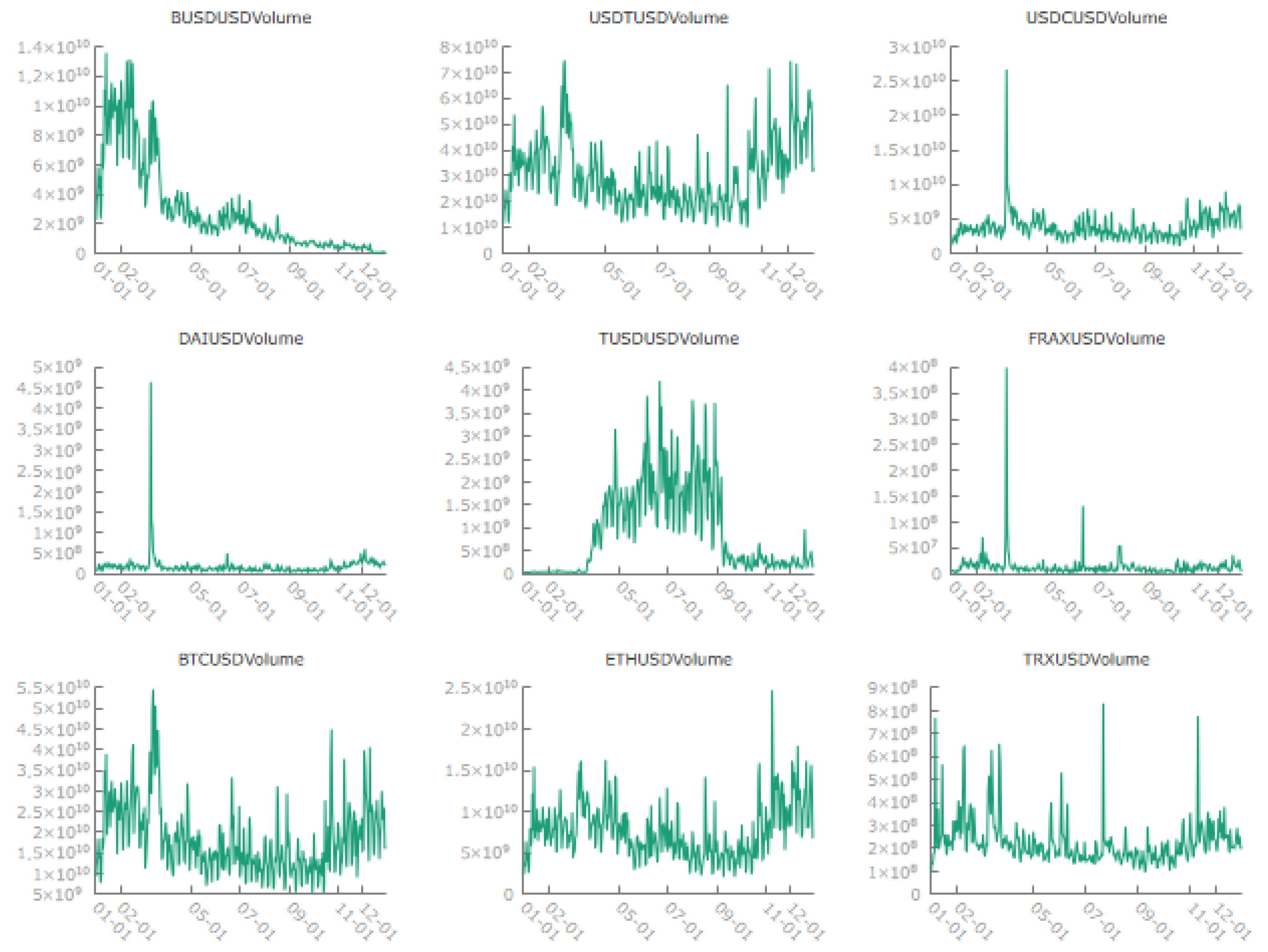
The graphs presented below provide key insights into the closing prices and trading volumes of leading cryptocurrencies and stablecoins during that year. In particular, Figure 1 examines stablecoins, including BUSD, USDT, USDC, DAI, TUSD, and FRAX. As expected, their prices are typically anchored around $1, though some, like USDC and TUSD, show temporary dips due to market instability or external factors. BUSD also experiences minor fluctuations but mostly maintains stability. Next, Figure 2 focuses on the closing prices of Bitcoin (BTC), Ethereum (ETH), and TRON (TRX). Bitcoin shows a general upward trend with notable fluctuations, particularly in the latter half of the year, indicating rising market confidence. Ethereum’s price closely follows Bitcoin’s trajectory, while TRON displays a more stable, gradual increase over the year. More precisely, Figure 3 illustrates trading volumes for stablecoins and major cryptocurrencies. High trading volumes for BUSD and TUSD at the year’s start decline over time, while USDT remains consistently high. BTC and ETH trading volumes spike in line with significant price movements, highlighting the relationship between trading activity and price volatility. TRX shows a more stable volume trend with occasional surges.

3.2. Identification and Dating of the BUSD Delisting Shock

The identification and dating of the BUSD delisting shock is a central element of our empirical strategy. We define this shock as a regulatory-driven event unfolding between February and mid-March 2023, with mid-March 2023 selected as the operational shock date in our Local Projections analysis.
The process was initiated on 13 February 2023, when the New York Department of Financial Services (NYDFS) issued a cease-and-desist order to Paxos Trust Company, requiring the immediate cessation of new BUSD token minting. This intervention followed regulatory warnings, widely reported by financial journalists, regarding Paxos’s oversight of its partnership with Binance, including concerns related to Anti-Money Laundering (AML) and Know Your Customer (KYC) compliance, as well as broader risk management practices. Concurrently, the U.S. Securities and Exchange Commission issued a Wells Notice to Paxos, signaling potential enforcement action concerning the legal classification of BUSD. These coordinated actions marked the formal regulatory origin of BUSD’s displacement from the stablecoin ecosystem.
We designate mid-March 2023 as the shock date because this is the period during which regulatory pressure translated into concrete and observable market adjustments. In particular, major cryptocurrency exchanges—including Coinbase—announced the suspension of BUSD trading, citing expected liquidity deterioration. Over the same period, BUSD’s market capitalization declined sharply as a result of both halted issuance and active redemptions, while trading volumes in BUSD pairs collapsed across platforms. Binance and other exchanges simultaneously encouraged users to migrate toward alternative stablecoins, most notably USDT and USDC. These developments indicate that mid-March represents the point at which the regulatory intervention crystallized into widespread market reallocation rather than a purely anticipatory response.
Several considerations support treating the BUSD delisting as exogenous to broader cryptocurrency market conditions. First, the shock originated from a targeted regulatory action aimed specifically at the Paxos–Binance arrangement, rather than from endogenous price dynamics or sector-wide stress. Second, our Markov-switching VAR analysis identifies a clear structural break in both price and volume dynamics around mid-March 2023, coinciding closely with the regulatory announcements and exchange delisting decisions. Third, the observed substitution patterns are highly concentrated: liquidity flows predominantly from BUSD toward USDT and USDC, rather than diffusing broadly across crypto assets, which is consistent with a BUSD-specific shock rather than a general market movement.
While other events occurred in early 2023—such as the temporary USDC depeg related to the Silicon Valley Bank episode and gradually evolving macroeconomic conditions—these factors either predate the main BUSD volume shifts or evolve too smoothly to account for the sharp and asset-specific breaks we document. Our lag-augmented Local Projections framework is designed to absorb such persistent influences while isolating short-run responses to identified shocks. Taken together, these elements justify treating the BUSD delisting as a distinct and identifiable regulatory shock in our empirical analysis.
Table 1 presents descriptive statistics for various cryptocurrency pairs, showing central tendency, dispersion, and distribution shape. It includes the Mean, Median, Minimum (Min), and Maximum (Max) values to display the range and central location of each variable. The Standard Deviation (Std. Dev.) and Coefficient of Variation (CV) are used to describe the spread and relative dispersion of the data. Skewness (Skew) and Kurtosis (Kurt) provide insights into the asymmetry and tail behavior of the distributions. Percentiles (5% and 95% P.) and Interquartile Range (IQR) give a more robust view of the data’s spread, while the Missing Observations count is included to highlight any data gaps. All volume figures are presented in millions.
In Table 1, the descriptive statistics from 2023 reveal key insights into cryptocurrencies and stablecoins. The closing prices of stablecoins like BUSD, USDT, USDC, DAI, TUSD, and FRAX show remarkable stability, with means and medians closely aligned with their pegged value of $1, and low standard deviations ranging from 0.0005 to 0.0024. However, occasional deviations from the peg are noted for USDC and DAI, indicated by high negative skewness and excess kurtosis, signaling rare depeg events. Trading volumes vary significantly, with USDT leading at a mean daily volume of 30,076 million. Bitcoin (BTC) and Ethereum (ETH) also demonstrate considerable activity, while USDC and BUSD maintain significant volumes. The volume data shows positive skewness and high kurtosis, highlighting occasional spikes, particularly in DAI and FRAX. Overall, while stablecoins largely uphold their pegs, the cryptocurrency market remains dynamic, marked by substantial trading volumes and extreme events. Descriptive statistics in logarithmic form can be found in Table A1 of the Appendix A.

3.3. Lag Selection for Local Projections

Brugnolini (2018) presents an innovative framework that utilizes information criteria to determine the optimal lag-length in Local Projections. In the realm of local projection (LP) methods for estimating impulse responses, the careful selection of the lag-length p is essential for achieving an appropriate balance between bias and variance. Following the methodology outlined by Brugnolini, this selection process incorporates information criteria, including the Akaike Information Criterion (AIC), Bayesian Information Criterion (BIC), Hannan–Quinn Criterion (HQC), and the Corrected Akaike Information Criterion (AICC). These criteria are designed to penalize model complexity while simultaneously rewarding goodness-of-fit, thereby ensuring a parsimonious model that does not sacrifice accuracy.

3.3.1. General Form of Information Criteria

For a model with p lags, the information criterion I C ( p ) is defined as:
I C ( p ) = ln σ ^ p 2 + c T · p T
where σ ^ p 2 is the estimated residual variance, T is the sample size, and c T is a penalty term specific to each criterion. The optimal lag-length p * minimizes I C ( p ) :
p * = arg min p P I C ( p )
with P denoting the set of candidate lag-lengths.

3.3.2. Specific Criteria

  • Akaike Information Criterion (AIC):
    The AIC imposes a penalty term c T = 2 :
    A I C ( p ) = ln σ ^ p 2 + 2 p T
    AIC favors larger lag-lengths to reduce bias but risks overfitting in small samples.
  • Bayesian Information Criterion (BIC):
    The BIC uses c T = ln ( T ) , penalizing complexity more severely:
    B I C ( p ) = ln σ ^ p 2 + ln ( T ) · p T
    BIC prioritizes parsimony, making it robust in small samples but potentially oversimplifying dynamics in larger datasets.
  • Hannan–Quinn Criterion (HQC):
    HQC employs c T = 2 ln ( ln ( T ) ) , intermediate between AIC and BIC:
    H Q C ( p ) = ln σ ^ p 2 + 2 ln ( ln ( T ) ) · p T
    This criterion balances bias–variance trade-offs, particularly effective in moderate sample sizes.

3.3.3. Application to Local Projections

In LP, impulse responses are estimated via horizon-specific regressions:
y t + h = α h + j = 1 p β h , j y t j + ε t + h , h = 1 , , H
For each horizon h, the lag-length p can be selected in two ways:
  • Fixed Lag-Length: Choose p * once (e.g., via BIC) and apply it uniformly across all horizons.
  • Horizon-Specific Lag-Length: Optimize p h * separately for each h, allowing flexibility but introducing variance.
The research conducted by Brugnolini (2018) illustrates that maintaining a fixed lag length p * across different horizons enhances the reliability of local projection models. This approach is particularly advantageous as horizon-specific optimization tends to amplify noise in finite samples. Findings from Monte Carlo experiments reveal that local projections (LPs) outperform vector autoregressive (VAR) models when there is lag length mispecification, especially when p * is selected using the Bayesian Information Criterion (BIC) or the Corrected Akaike Information Criterion (AICC), with pronounced benefits in smaller sample sizes.

3.3.4. Practical Considerations in Lag-Length Selection

The selection of lag length in local projection models embodies a critical trade-off between bias and variance, exhibiting sensitivity to sample size. In smaller samples, stringent penalty terms found in criteria such as the BIC and AICC effectively mitigate overfitting by favoring more parsimonious model specifications. These criteria lower variance at the expense of potential bias, which proves advantageous when the threat of model saturation outweighs the benefits of enhanced dynamic complexity. Conversely, in larger datasets, the use of the Akaike Information Criterion (AIC) and the Hannan–Quinn Criterion (HQC) is more appropriate, as these criteria impose lighter penalties, accommodating more intricate dynamics and capturing subtle interactions that simpler models might overlook.
Following Jordà (2005) and the lag-augmented Local Projections framework of Montiel Olea and Plagborg-Møller (2021), our baseline specification includes one lag of the dependent variables and controls to balance dynamic adequacy and parsimony. We verify that the estimated impulse responses are robust to alternative lag lengths, projection horizons, and reasonable variations in heteroskedasticity- and autocorrelation-consistent standard errors, with no material changes in their sign, timing, or economic interpretation.
Local projection methods possess inherent robustness to lag length misspecification when compared to VAR models, attributed to their horizon-specific regression framework. This robustness is a result of the decoupling of horizon estimates, which limits the propagation of error across time periods. Nevertheless, this characteristic does not diminish the necessity for careful selection of lag length, as suboptimal choices can distort impulse response estimates and compromise the validity of inferences. Consequently, researchers are advised to strike a balance between theoretical assumptions regarding the data-generating process and evidence-based criteria, ensuring that lag lengths align with both empirical findings and economic theory. Fixing a uniform lag length across all horizons, rather than optimizing for each horizon individually, often enhances reliability by reducing estimation noise, particularly in finite samples. This strategy stabilizes the trade-off between flexibility and precision, consistent with Monte Carlo evidence that underscores the superiority of BIC and AICC in small-sample applications of local projections.

3.3.5. Application to BUSD Data

When running the lag-length selection procedure by Brugnolini (2018) to our data composed of BUSD and eight other cryptocurrencies, we obtain the following result:
  • AIC suggests 2 lags.
  • BIC suggests 1 lags.
  • HQC suggests 1 lags.
The same results apply for price series and volume series (in log form). For parsimony, we proceed with estimating Local Projections with one lag in this paper.

4. Linear Local Projections

The econometric analysis is structured into three distinct steps. First, linear local projections are computed using price series expressed in logarithmic form. Second, we regenerate the linear local projections utilizing volume data, also in logarithmic form, to facilitate a comparative analysis of the results. Lastly, we introduce a VAR(1) model to serve as a benchmark for this study.

4.1. Linear Price Analysis

This section provides the estimated impulse response functions (IRFs) obtained through the Local Projections (LPs) method. The purpose of this analysis is to evaluate how the prices of key stablecoins in our dataset respond to a shock in the closing price of BUSD. The responses are examined over a 12-period horizon, and confidence intervals are included to illustrate the statistical significance of the results.
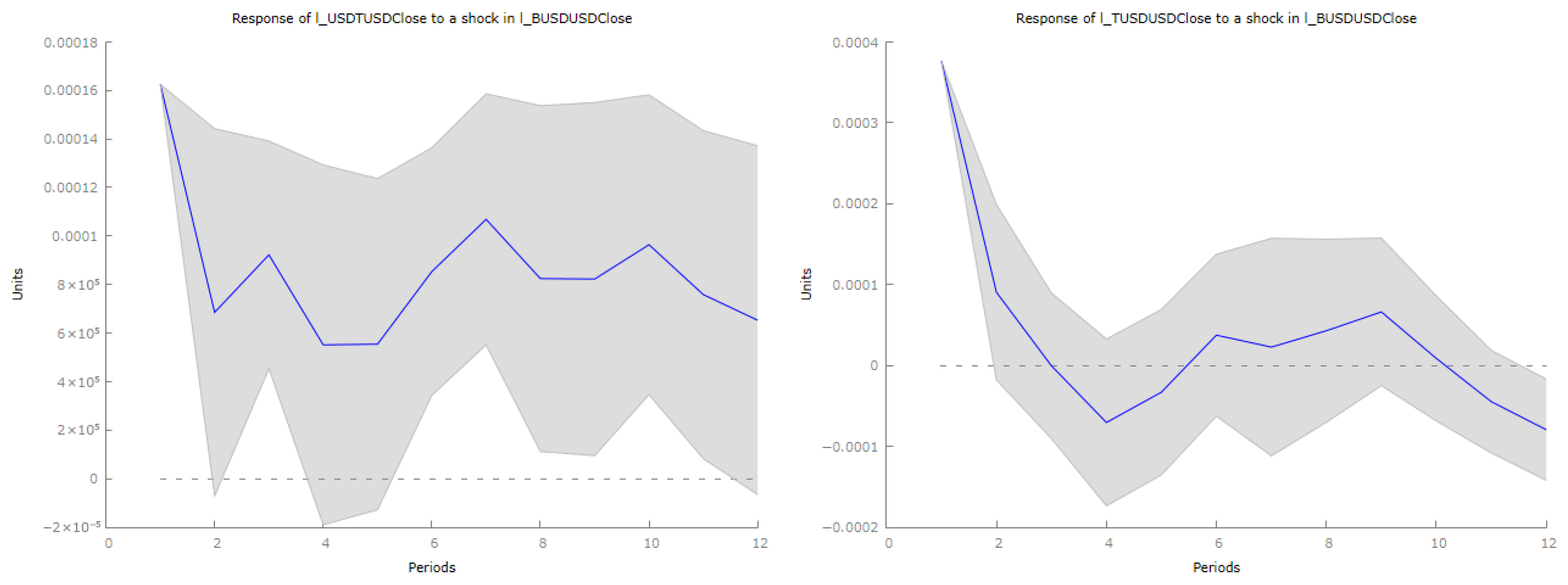
The impulse response functions illustrated in Figure 4 reveal several significant patterns pertaining to the cross-elasticity of stablecoin prices, suggesting intricate interconnections within the digital currency ecosystem. Notably, USDT displays characteristics that align with the “flight-to-quality” phenomenon commonly observed in traditional financial markets. The immediate positive price elasticity ( β 0 ) following a BUSD shock, in conjunction with rapid mean reversion, indicates a sophisticated market mechanism wherein temporary arbitrage opportunities are swiftly eliminated. This outcome is consistent with theoretical predictions derived from established market efficiency models within digital asset markets. The rapid attenuation of the effects (as time approaches zero following initial periods) provides empirical support for the hypothesis that dominant stablecoins possess robust price stability mechanisms, likely attributable to superior market depth and liquidity networks.
The response function of TUSD offers a compelling case study regarding the dynamics of second-tier stablecoins. The initial positive elasticity followed by a decay suggests a temporal hierarchy in cross-stablecoin substitution effects. This phenomenon can be interpreted through the lens of limited arbitrage capital theory, which posits that smaller market participants encounter constraints that limit their capacity for sustained capital reallocation. The parameters of the decay function imply that considerations of market depth supersede short-term substitution effects in establishing long-term equilibrium.
In Figure 5, the response pattern of USDC is particularly noteworthy due to its non-monotonic features. The initial positive shock, followed by a negative adjustment phase, indicates the presence of complex feedback mechanisms within the stablecoin ecosystem. This finding challenges the prevailing assumption of uniform substitution effects among stablecoin pairs and suggests the possibility of strategic complementarities within digital asset markets. The observed pattern may be rationalized through a model of sequential portfolio rebalancing, whereby institutional investors optimize their holdings of stablecoins across various time horizons.
Concerning alternative cryptocurrencies, the findings for TRON merit careful consideration. The observed delayed positive response (approximately two weeks) suggests potential spillover effects within the trading ecosystem rather than direct price correlations. This temporal lag structure may reveal second-order effects emerging from market microstructure channels.
In Figure 6, the absence of significant responses in FRAX, BTC, and ETH lends empirical support to the market segmentation hypothesis within cryptocurrency markets. This finding bears important implications for portfolio diversification strategies and indicates that the stablecoin market retains a degree of isolation from the broader dynamics of cryptocurrency prices.
These results contribute to a deeper understanding of price formation mechanisms in digital asset markets and suggest several avenues for future research, particularly regarding the role of market microstructure in influencing cross-asset price dynamics.

4.2. Linear Volume Analysis

This section examines the effects of BUSD volume shocks on the trading activity of major stablecoins and cryptocurrencies, employing a Vector Autoregression (VAR) framework. Analyzing volume dynamics offers valuable insights into how liquidity flows adjust in response to fluctuations in BUSD trading activity, thereby revealing potential substitution effects between stablecoins and spillover effects on the broader cryptocurrency markets. Given the essential role of stablecoins in facilitating market liquidity, understanding these volume interactions is critical for assessing the extent to which changes in BUSD trading influence the stability and liquidity of other digital assets. The findings underscore the significant roles of USDT and USDC in absorbing displaced liquidity, highlight the comparatively weaker responses of decentralized and algorithmic stablecoins, and illustrate the broader market implications for the trading activities of Bitcoin and Ethereum.
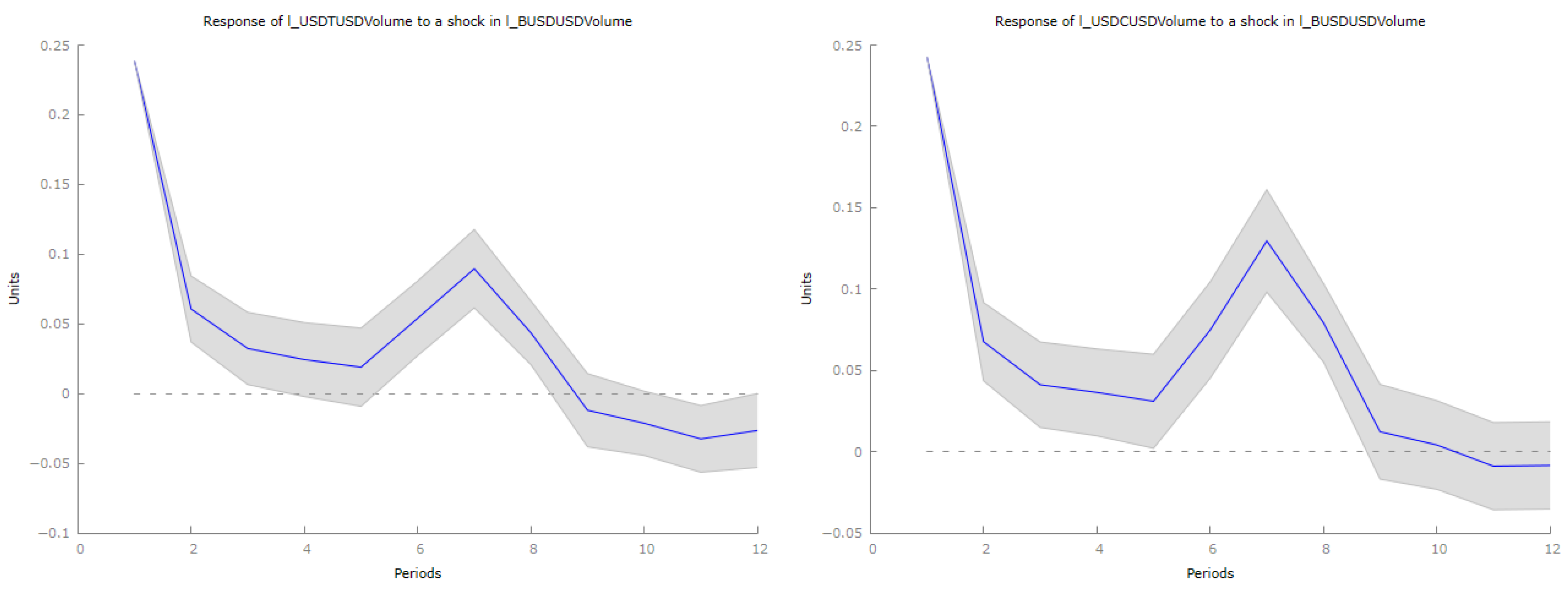
To quantify the net migration of trading activity following the BUSD delisting, we examined the impulse responses of stablecoin volumes to a BUSD-specific shock. As shown in Figure 7, the results indicated that BUSD volume contractions are associated with economically meaningful but transitory reallocations toward USDT and USDC, whereas responses for DAI, FRAX, and TUSD remain quantitatively limited. Importantly, these reallocations are large relative to BUSD’s own baseline liquidity but small in percentage terms relative to the substantially larger trading volumes of USDT and USDC, indicating targeted substitution effects rather than broad-based increases in market-wide trading activity.
To assess whether these patterns simply reflect aggregate liquidity fluctuations, the Local Projections are estimated in a multivariate system that conditions on the joint dynamics of major stablecoins and large cryptocurrencies (BTC, ETH, TRX). This specification absorbs common market-wide volume shocks and slowly evolving liquidity conditions through the lag structure. Once these dynamics are controlled for, the BUSD-specific innovation continues to generate short-run, asset-specific reallocations toward USDT and USDC, with no evidence of persistent volume effects beyond the immediate adjustment horizon. This supports the interpretation of the documented migration as a temporary and targeted response to the BUSD delisting, rather than a manifestation of generalized market-wide volume shifts.
In Figure 8, the impulse response function of USDT trading volume following a positive shock in BUSD volume shows a strong initial spike, indicating that traders promptly shift from BUSD to USDT as an alternative stablecoin. This suggests USDT captures significant displaced trading activity. After this initial increase, the response gradually declines, with a temporary secondary rise around the sixth period, likely reflecting delayed market adjustments. Ultimately, USDT volume declines further, indicating the transient nature of this liquidity migration.
Similarly, USDC exhibits an immediate positive response following a BUSD shock, confirming it as an alternative stablecoin. Like USDT, USDC’s initial increase diminishes over time with a similar secondary peak, suggesting rebalancing strategies among traders. However, it also transitions to negative values later, indicating that while it temporarily absorbs displaced BUSD volume, this effect is short-lived.
Overall, both USDT and USDC emerge as primary alternatives to BUSD during trading volume declines, reflecting their dominant positions in the stablecoin market. The observation of secondary peaks indicates liquidity shifts occur in waves due to trading algorithms and market frictions. Long-term declines in USDT and USDC volumes suggest that liquidity reallocation is temporary, reverting to equilibrium as market conditions stabilize.
From a regulatory standpoint, these findings illustrate the interconnected nature of stablecoins and how regulatory actions affecting one can lead to short-term liquidity migrations to others. However, such reallocations are not lasting, highlighting the importance of sustained market confidence in regulatory frameworks for long-term stability. Disruptions in BUSD trading prompt significant but short-lived liquidity reallocations toward USDT and USDC, emphasizing the need to monitor trading volume flows in assessing stablecoin resilience.
The impulse response functions (IRFs) in Figure 9 shed light on how DAI and FRAX respond to changes in BUSD liquidity, as well as the behavior of other stablecoins. The analysis reveals that FRAX, which has a unique stabilization mechanism, shows a moderate and temporary increase in trading volume following a positive shock in BUSD trading volume. However, this response is weaker than that of USDT and USDC, indicating that FRAX is not a primary refuge for liquidity during market disruptions.
Following the initial increase, FRAX trading volume declines and eventually turns negative, suggesting that traders revert to other stablecoins rather than maintaining positions in FRAX. In contrast, DAI’s response to a BUSD shock also reflects a positive trend initially, yet its volume response is characterized by fluctuations rather than a strong shift. This variability in DAI’s trading volume may stem from its dual nature as a decentralized and partially fiat-collateralized stablecoin, leading to more irregular liquidity adjustments.
Similar to FRAX, DAI’s trading volume response becomes negative over time, indicating that liquidity reallocations are not permanent. Overall, both FRAX and DAI demonstrate weaker and more transient responses compared to USDT and USDC, highlighting that they are not primary alternatives during market stress. The results suggest that the challenges faced by algorithmic stablecoins in attracting liquidity during disruptions stem from concerns regarding stability and market adoption.
Liquidity remains concentrated among dominant stablecoins like USDT and USDC, which capture most trading volumes during disruptions. This implies that significant fluctuations predominantly affect major fiat-backed assets rather than decentralized stablecoins. The fleeting nature of liquidity shifts indicates that market confidence is more reliant on liquidity depth and regulatory clarity than on the stabilization mechanisms of individual stablecoins.
Figure 10 analyzes the dynamic response of trading volumes for TRX, TUSD, BTC, and ETH following a shock to BUSD trading volume. The impulse response functions (IRFs) reveal how different asset classes respond to changes in BUSD liquidity, shedding light on market-wide spillover effects and the roles of individual assets in managing displaced liquidity.
TRX trading volume initially surges in response to the BUSD shock, indicating liquidity reallocation towards this transactional cryptocurrency, especially within DeFi applications. However, this increase is short-lived, followed by a decline as liquidity adjustments occur in waves, potentially due to market frictions or delayed decisions.
TUSD also shows an initial increase in trading volume after the shock, suggesting temporary liquidity shifts from BUSD. Yet, the magnitude of this response is weak, indicating that TUSD is not viewed as a long-term alternative to BUSD. The transient spike may reflect speculative activity, and as the market stabilizes, liquidity reallocates to dominant stablecoins like USDT and USDC.
In contrast, BTC experiences a sustained negative response post-shock, with a decline in trading volume indicating reduced overall market liquidity, which supports the notion that stablecoin liquidity is vital for market efficiency. A similar declining pattern is observed with Ethereum, revealing its strong dependency on stablecoin liquidity, especially in DeFi contexts. This decline underscores systemic liquidity risks in the broader cryptocurrency market.
Overall, the findings highlight the varying reactions of different asset classes to changes in BUSD trading volume, reflecting complex interactions within the cryptocurrency ecosystem.

4.3. Implications for Systemic Stability: Resilience of Bitcoin and Ethereum

The response of Bitcoin (BTC) and Ethereum (ETH) to the BUSD delisting provides additional insights into systemic stability and shock-absorption mechanisms within cryptocurrency markets. While stablecoin disruptions generate short-term liquidity stress, the behavior of these core crypto-assets suggests a degree of resilience that contrasts with the more persistent dislocations observed for smaller cryptocurrencies and algorithmic stablecoins.
Our impulse response analysis reveals a common dual-phase adjustment pattern for both BTC and ETH. In the immediate aftermath of the BUSD delisting, trading volumes decline significantly, with short-run contractions on the order of 15–25% across specifications. This initial response reflects a temporary tightening of market-wide liquidity conditions as the disruption to BUSD trading pairs constrains settlement and arbitrage activity. Importantly, this contraction is short-lived. Within approximately two to three weeks, trading volumes gradually recover toward pre-shock levels, indicating a restoration of market functioning rather than persistent impairment.
This recovery distinguishes BTC and ETH from assets that exhibit weaker or delayed adjustment following the shock. The differential response suggests that the largest cryptocurrencies possess structural characteristics that enhance their capacity to absorb stablecoin-related liquidity disturbances. In particular, BTC and ETH benefit from deep and geographically diversified liquidity pools, multiple trading pairs (including USDT, USDC, and fiat pairs), and active cross-exchange arbitrage mechanisms. As liquidity migrates away from BUSD toward alternative stablecoins, these assets are able to rapidly re-establish effective trading infrastructure.
Fundamental considerations also play a role. The valuation of Bitcoin as a store of value and Ethereum’s position as the dominant smart-contract platform are driven primarily by network effects, technological adoption, and institutional participation rather than dependence on any single stablecoin. While stablecoins are critical for facilitating trading and liquidity provision, they do not constitute the primary source of value for these assets. This relative independence helps explain why BTC and ETH recover more quickly once alternative liquidity channels become operational.
From a systemic perspective, these findings suggest a layered structure of resilience within the cryptocurrency ecosystem. Stablecoin concentration clearly introduces vulnerabilities at the infrastructure level, as evidenced by the sharp but temporary liquidity contraction following the BUSD delisting. However, the ability of core crypto-assets to adapt through liquidity reallocation indicates that increased stablecoin concentration does not mechanically translate into immediate instability of the broader market. Instead, systemic risk appears to depend on the joint disruption of multiple layers, including the availability of credible stablecoin substitutes.
At the same time, the observed resilience should not be overstated. The initial contraction phase highlights the continued reliance of BTC and ETH on stablecoin-mediated liquidity, and the recovery documented here occurs in an environment where alternative stablecoins (USDT and USDC) remained operational and credible. More severe scenarios—such as simultaneous disruptions affecting multiple major stablecoins or coincident macro-financial stress—could lead to materially different outcomes.
Overall, the response of Bitcoin and Ethereum to the BUSD delisting complements our earlier findings on stablecoin substitution and concentration. It underscores that while stablecoin regulation has important implications for market liquidity and infrastructure, the core cryptocurrency markets exhibit meaningful, though conditional, shock-absorption capacity.

4.4. VAR Benchmark Model

We construct a VAR model utilizing log-differenced series to enhance our analysis, as local projections provide a counterpart to VAR models. The findings in Table 2 and Table 3 indicate the importance of maintaining a low number of lags. In pursuit of parsimony, we select p = 1 in accordance with the Bayesian Information Criterion (BIC).
Table 4 presents the results of the Vector Autoregression (VAR) model, which has been estimated on the log-differenced price series of the selected assets. This analysis effectively captures the short-term dynamics and interdependencies between BUSD, other stablecoins, and prominent cryptocurrencies.
Table 5 presents the results of the VAR model estimated on the log-differenced trading volumes of BUSD, other stablecoins, and major cryptocurrencies. This model captures the short-term dynamics and liquidity interactions between these assets, yielding valuable insights into how changes in trading activity propagate throughout the market.
The estimated coefficients illustrate the extent to which past volume changes in one asset influence current trading volumes in other assets. A positive and statistically significant coefficient suggests that an increase in the trading volume of one asset leads to an increase in another asset’s trading volume, whereas a negative coefficient signifies an inverse relationship. The results indicate that fluctuations in BUSD trading volume have a significant impact on the trading volumes of other stablecoins, particularly USDT and USDC, thereby confirming their role as primary substitutes during liquidity shifts. The effect on decentralized and algorithmic stablecoins, such as DAI and FRAX, appears comparatively weaker, suggesting that traders reallocate liquidity to these assets less frequently.
In the case of major cryptocurrencies like BTC and ETH, the response to changes in BUSD trading volume is more complex. The coefficients imply that reductions in stablecoin trading volume correlate with diminished liquidity in the broader cryptocurrency market, thus reinforcing the importance of stablecoins as facilitators of trading activity. The autoregressive terms indicate that liquidity shocks endure over multiple periods, signifying that changes in trading volume do not dissipate immediately but rather continue to affect market conditions over time.
These findings underscore the critical role of stablecoins in sustaining overall market liquidity and indicate that disruptions in their trading volumes may have systemic implications. The results offer significant insights for market stability, liquidity management, and regulatory oversight, particularly with regard to potential restrictions on stablecoin utilization or delistings.
Diagnostic tests are proposed in Table A2 and Table A3 located in Appendix A.

5. Nonlinear Local Projections

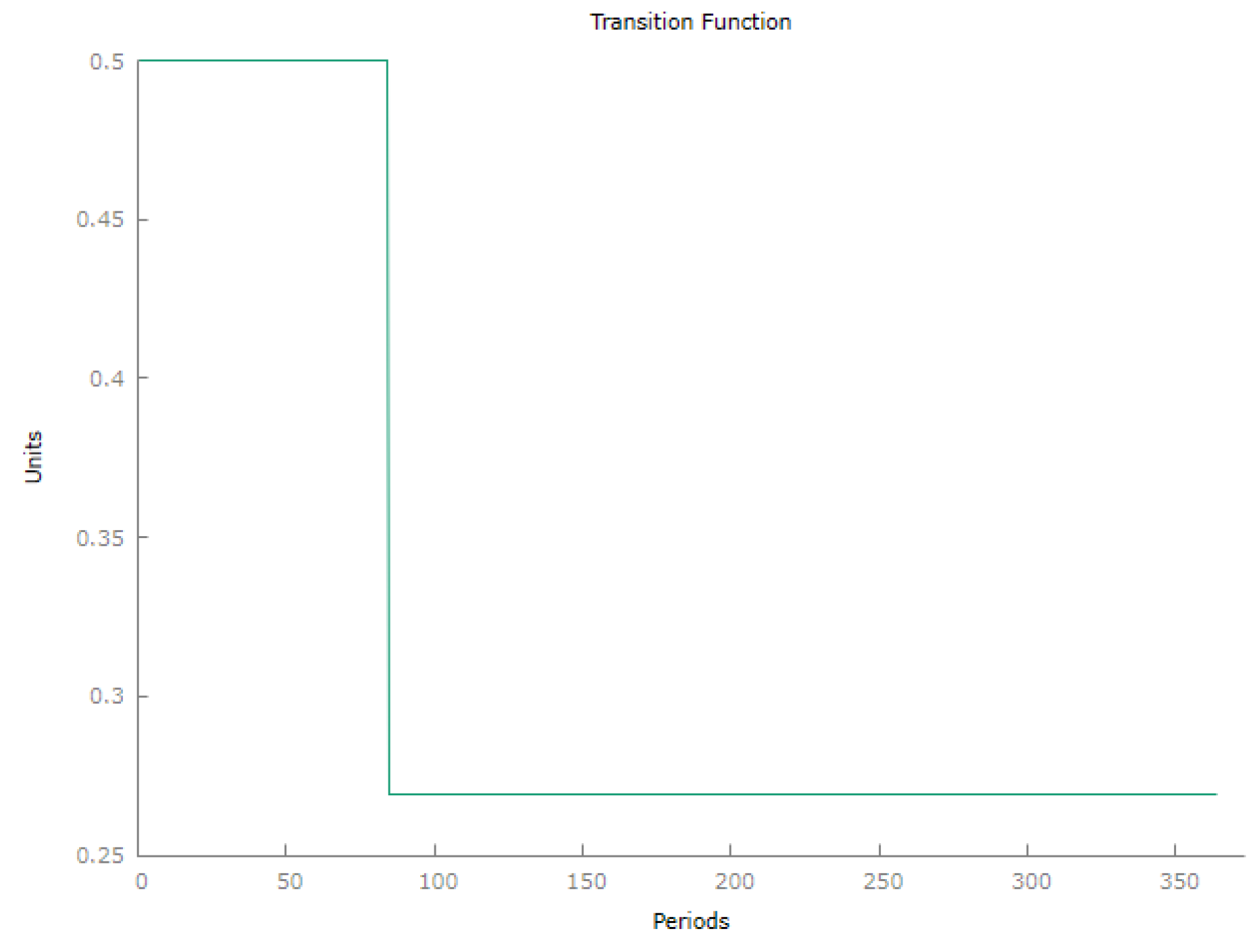
Based on contemporaneous regulatory and market developments, we designate mid-March, 2023 as the trigger date for the transition function. In particular, by mid-March, Coinbase had formally announced the suspension of BUSD trading (effective 13 March) citing liquidity concerns1. BUSD’s market capitalization had already dropped below USD 10 billion in reaction to regulatory pressure and withdrawal activity. This temporal proximity to observable shifts in volumes justifies using mid-March as the threshold for regime change in our nonlinear local projection model.
In Figure 11, the transition function behaves similarly to a step function, enabling the classification of regimes in which BUSD operates, contingent upon the underlying data.

5.1. Nonlinear Price Analysis

This section analyzes the effects of BUSD price shocks on major stablecoins and cryptocurrencies using nonlinear local projections. By examining how asset prices respond to BUSD fluctuations, we reveal asymmetric market dynamics and substitution patterns within the stablecoin ecosystem.

5.1.1. Dominant Stablecoins: Flight-to-Quality Effects

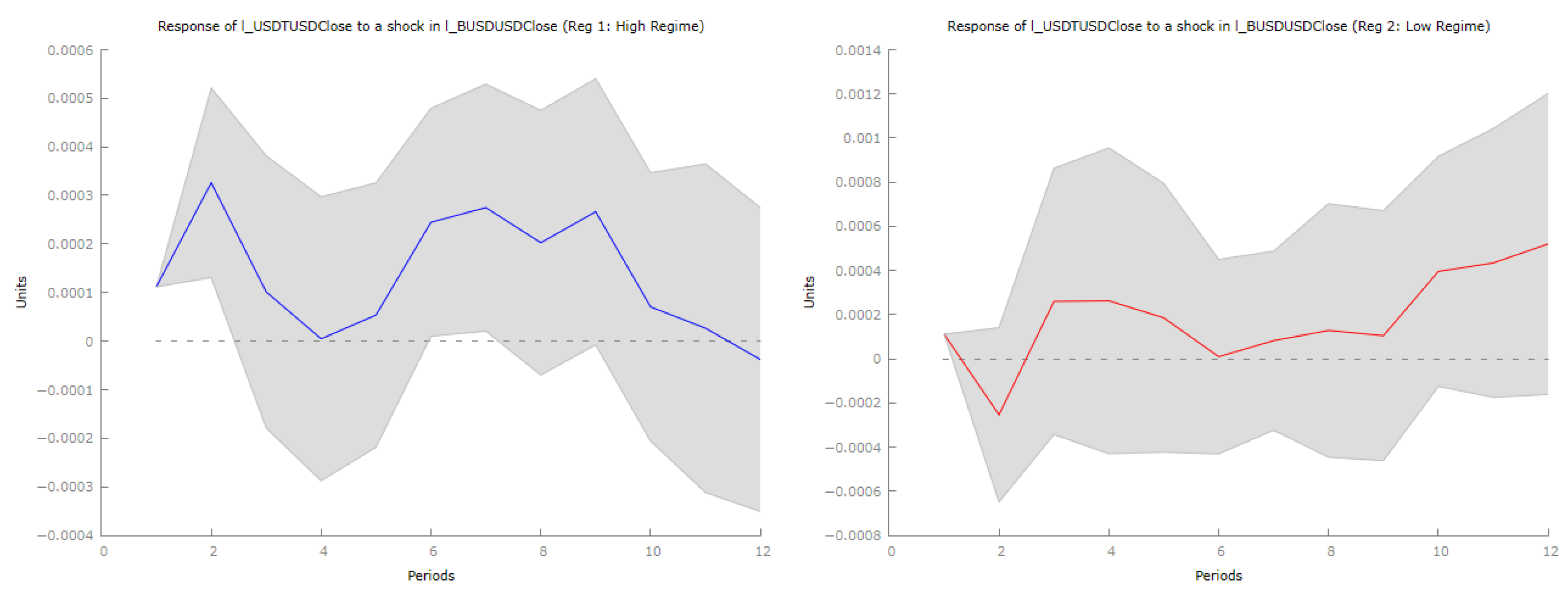
Figure 12 reveals that USDT exhibits strong asymmetric responses to BUSD shocks, with pronounced reactions during market stress periods. Initially, USDT prices rise as traders shift liquidity from BUSD, reinforcing its role as the leading stablecoin. This response is more pronounced during high-stress conditions, demonstrating a clear “flight-to-safety” pattern. The gradual correction following initial spikes suggests market stabilization over time, with confidence intervals indicating significant short-term effects but muted long-term impacts.
USDC shows in Figure 13 strong initial responses during market distress, with traders seeking it as a reliable alternative amid BUSD volatility. The response is more muted during stable conditions, indicating that BUSD price fluctuations have limited impact unless perceived risk increases. Short-term data reveal notable price increases as capital shifts from BUSD, aligning with USDC’s reputation for regulatory compliance and transparency. The response normalizes over time, reflecting market stabilization after shocks.
These findings highlight that fiat-backed stablecoins (USDT and USDC) effectively absorb displaced liquidity during BUSD disruptions, with market confidence concentrated in established, regulated alternatives.

5.1.2. Secondary and Decentralized Stablecoins: Limited Absorption Capacity

In Figure 14, DAI exhibits volatile and unpredictable responses compared to dominant stablecoins. While showing slight initial positive reactions during market stress, its response is less pronounced due to its hybrid decentralized nature. The response pattern features oscillations rather than clear trends, suggesting uncertainty about DAI’s role as a safe haven. Broader confidence intervals indicate greater uncertainty compared to fiat-backed alternatives, revealing that DAI does not effectively absorb liquidity shocks in the stablecoin market.
As can be observed in Figure 15, TUSD initially reacts positively to BUSD volatility as traders temporarily shift funds to this fiat-backed alternative. However, this response is weaker than USDT and USDC, indicating TUSD’s limited role as a dominant substitute. Over time, TUSD’s response stabilizes but exhibits fluctuations, pointing to unpredictable market reactions and widening confidence intervals that suggest increased investor uncertainty.
Figure 16 reveals that FRAX demonstrates weak and inconsistent responses to BUSD shocks, indicating it is not viewed as a primary substitute during market instability. Unlike fully fiat-backed stablecoins, FRAX’s hybrid algorithmic structure contributes to investor uncertainty. The response lacks clear trends and remains volatile, reflecting doubts about long-term stability. This underscores challenges faced by algorithmic stablecoins during uncertain periods.

5.1.3. Traditional Cryptocurrencies: Dual-Phase Recovery Patterns

In Figure 17, Bitcoin (BTC) reacts asymmetrically to BUSD shocks, reflecting its dual role as both speculative asset and liquidity haven. Initially, BTC shows slight negative responses during market stress, indicating reduced cryptocurrency market confidence and liquidity concerns. However, this is followed by positive adjustment as investors view BTC as a store of value amid stablecoin instability. This dual-phase pattern aligns with Bitcoin’s historical role as a hedge against uncertainty, with the response stabilizing in the medium to long term.
Ethereum (ETH) displays asymmetric responses with initial moderate negative reactions in Figure 18, suggesting that BUSD instability undermines confidence in crypto market liquidity. Given Ethereum’s reliance on stablecoin liquidity for DeFi activities, BUSD disruptions temporarily hinder lending, borrowing, and trading on Ethereum protocols. Over time, ETH’s response shifts positive as investors rebalance portfolios, indicating that while BUSD disruptions create initial uncertainty, Ethereum retains its appeal. The response eventually stabilizes, suggesting adaptation to stablecoin fluctuations.
In Figure 19, TRON (TRX) shows dynamic asymmetric responses with modest initial price increases as market participants view it as an alternative during BUSD variability. However, this response diminishes over time, reflecting market corrections. The medium to long-term stabilization suggests temporary price effects from BUSD shocks, with increased uncertainty influenced by regulatory changes and network activity factors.

5.2. Nonlinear Volume Analysis

This section investigates how BUSD volume shocks affect trading activities across stablecoins and cryptocurrencies using nonlinear local projections. Understanding volume dynamics reveals liquidity reallocation patterns, substitution effects, and broader market implications during stablecoin disruptions.

5.2.1. Primary Liquidity Absorbers: USDT and USDC Dominance

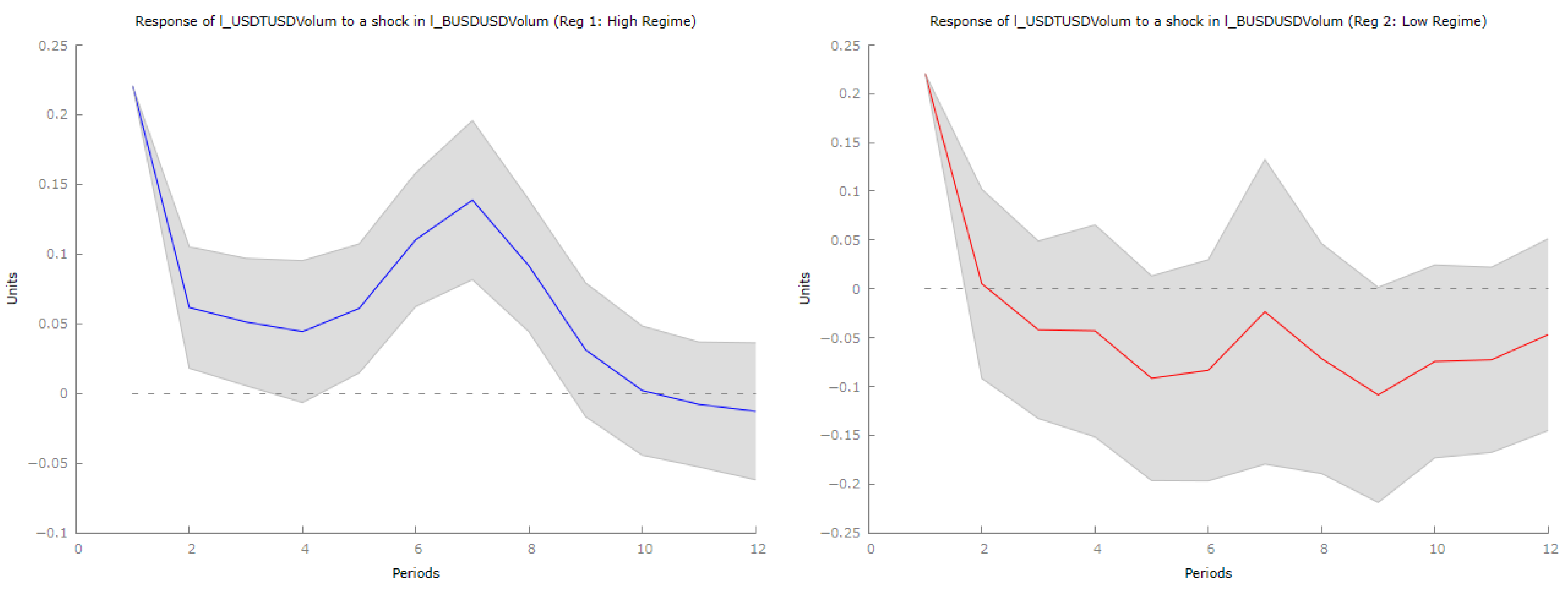
Figure 20 unveils that USDT demonstrates the strongest asymmetric response to BUSD volume shocks, reinforcing its role as the primary liquidity absorber. Following positive BUSD shocks, USDT volume surges significantly, reflecting market perception of USDT as the most stable alternative. This response is amplified under high-stress conditions, demonstrating a clear “flight-to-safety” pattern. The initial volume increase is followed by gradual decline as market conditions normalize, but USDT retains its status as the preferred trading pair for most crypto assets.
In Figure 21, USDC shows strong but slower responses compared to USDT, with gradual increases in trading volume following BUSD shocks. This measured response reflects USDC’s positioning as a regulated, transparent alternative preferred by institutional investors. The response is more pronounced during market stress, highlighting USDC’s role as a stability-seeking asset. Liquidity reallocations occur in stages, influenced by risk assessments and regulatory considerations, with effects diminishing as conditions stabilize.
Both dominant stablecoins effectively capture displaced BUSD liquidity, with USDT providing immediate absorption and USDC offering institutional-grade stability. This concentration pattern reinforces existing market hierarchies while potentially increasing systemic risks.

5.2.2. Secondary and Algorithmic Stablecoins: Limited Market Appeal

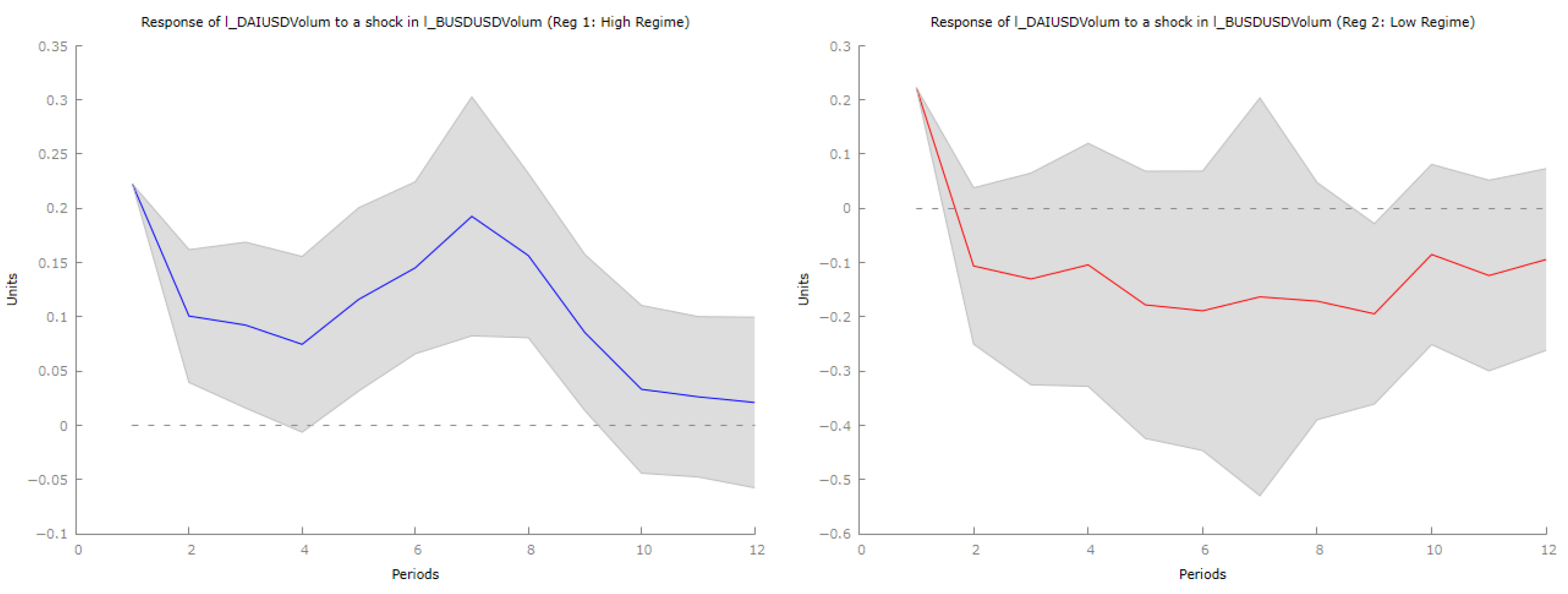
As can be observed in Figure 22, DAI exhibits weak and irregular responses to BUSD volume shocks, indicating minimal role in liquidity reallocation. While showing slight initial upticks, these are minimal compared to USDT and USDC responses. The inconsistent oscillatory behavior reflects market uncertainty about DAI’s decentralized, crypto-collateralized structure. Under high-stress conditions, DAI sees marginal liquidity increases, but these pale compared to fiat-backed alternatives, reinforcing its secondary market position.
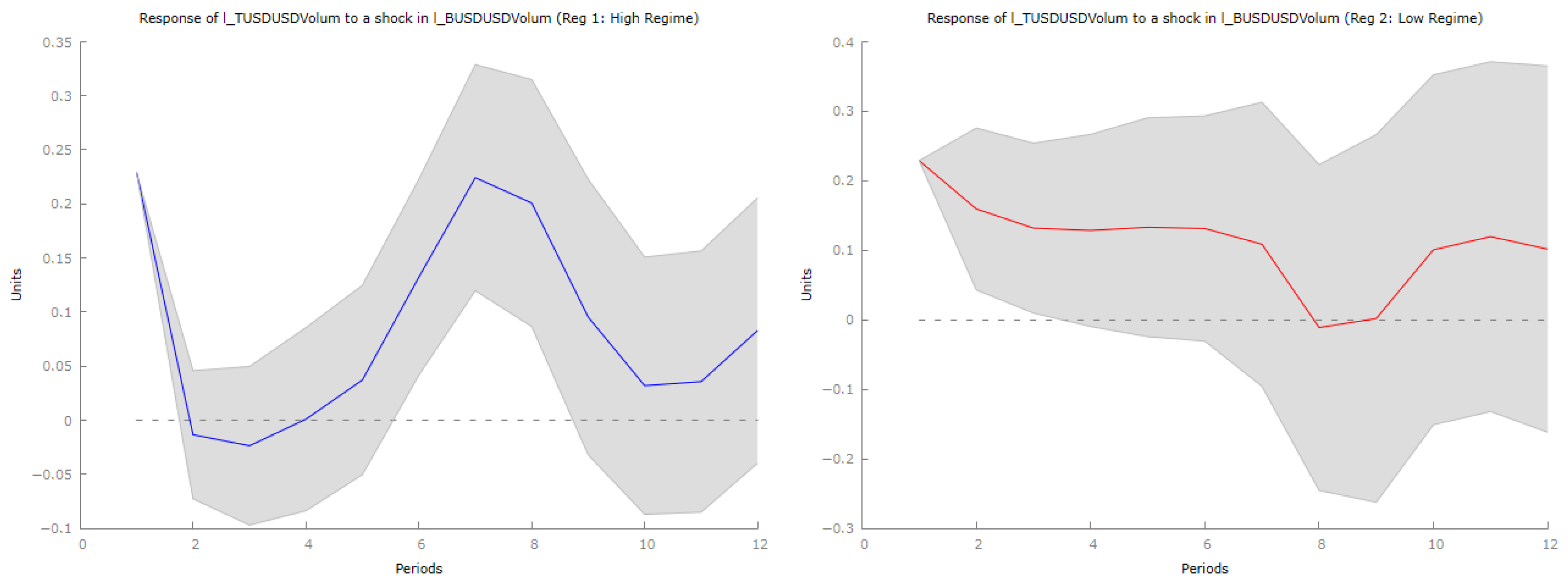
In Figure 23, TUSD initially increases following BUSD shocks as traders view it as a temporary fiat-backed substitute. However, this response is short-lived and significantly weaker than dominant stablecoins. The trading volume reverts to equilibrium over time, confirming TUSD’s limited role as a long-term BUSD alternative. While more pronounced under market stress, TUSD lacks the liquidity depth and market dominance necessary for sustained substitution.
FRAX demonstrates in Figure 24 the weakest response among stablecoins, showing only minor volume increases that reflect limited market confidence in algorithmic mechanisms during stress periods. The oscillatory volume behavior suggests irregular liquidity shifts influenced by market volatility and algorithmic adjustments. FRAX remains a secondary option for liquidity reallocation, underscoring challenges faced by non-fiat-backed stablecoin designs.
The limited capacity of secondary and algorithmic stablecoins to absorb displaced liquidity highlights structural vulnerabilities in non-fiat-backed designs and reinforces market preference for established, regulated alternatives.

5.2.3. Traditional Cryptocurrencies: Interconnected Liquidity Dependencies

Figure 25 illustrates that Bitcoin (BTC) trading volume experiences moderate initial decline following BUSD shocks, indicating that stablecoin disruptions temporarily reduce overall market liquidity. This decline is followed by gradual rebound, suggesting Bitcoin’s capacity to recover as traders reallocate liquidity. The oscillatory pattern reflects dynamic relationships influenced by market sentiment and macroeconomic factors. Under high-stress conditions, BTC shows more pronounced responses to stablecoin liquidity contractions, demonstrating vulnerability to stablecoin market disruptions.
Ethereum (ETH) displays asymmetric and dynamic responses in Figure 26, with initial volume declines reflecting its integration within DeFi ecosystems and dependence on stablecoin liquidity. The temporary contraction in trading activity likely stems from reduced liquidity in DeFi platforms that rely heavily on stablecoins. However, ETH demonstrates resilience through eventual volume recovery, indicating adaptation as traders adjust positions. The oscillatory characteristics suggest liquidity adjustments unfold over time through automated trading and DeFi rebalancing mechanisms.
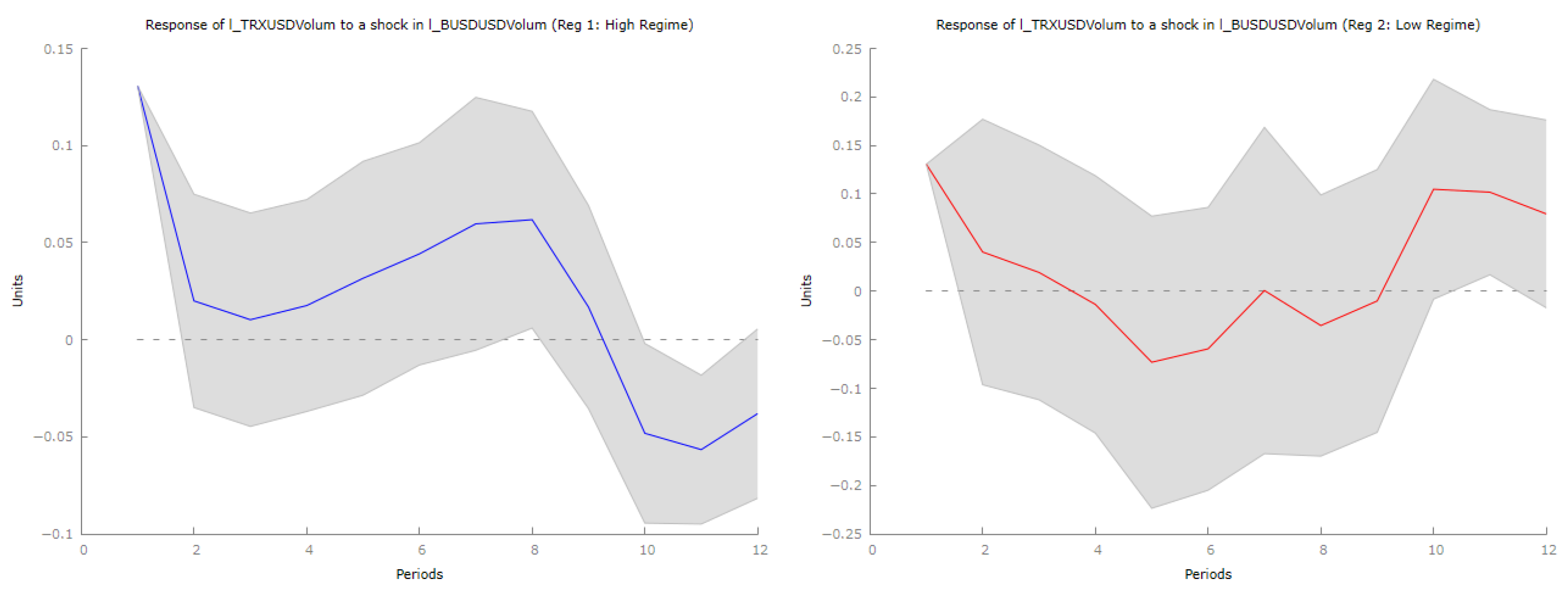
In Figure 27, TRON (TRX) shows asymmetric but temporary responses to BUSD volume fluctuations, with short-term positive reactions as some traders increase TRX activity. This suggests TRX absorbs limited displaced liquidity, particularly in stablecoin-related transactions. However, increases are not sustained and decline shortly after shocks, with oscillatory patterns indicating wave-like liquidity adjustments. Under stress conditions, responses are slightly more pronounced but remain significantly smaller than dominant stablecoins.

5.3. Regime-Switching Benchmark Model

5.3.1. Price Series

As a benchmark for nonlinear Local Projections, this analysis employs a two-regime Markov-switching vector autoregression (VAR) model with one lag.
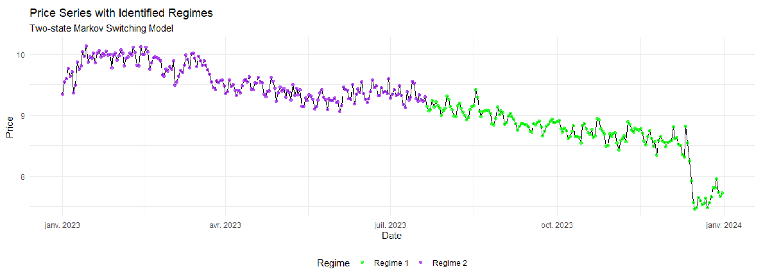
As can be glanced by looking at Figure 28, the results demonstrate a successful identification of regimes in both price and volume series, consistent with traditional econometric practices. Notably, a predominant number of transitions from regime 1 (low) to regime 2 (high) occurred during March 2023, coinciding with communications from U.S. attorneys to Binance regarding the upcoming delisting of BUSD by the end of the year. Consequently, the market has begun to price this information in advance, anticipating the removal of BUSD and its subsequent replacement with alternative stablecoins later in the year. In contrast, the Local Projections framework offered different perspectives.
In Table 6, the values of the transition function illustrating the movement between different regimes are presented, as depicted previously. The analysis demonstrates that these regimes exhibit stability; once the model transitions into a specific regime, it typically remains within that regime for several months. Notable deviations from this stability occur following the announcement of BUSD’s delisting and during the transition period when BUSD is replaced with alternative stablecoins.

5.3.2. Volume Series

In concluding this analysis, we proceed to the estimation of a two-state Markov regime-switching model for BUSD volumes (in logarithmic form) alongside eight other cryptocurrencies, which will serve as benchmarks for our Nonlinear Local Projections.
In Figure 29, the results indicate substantially greater stability in the volumes. Notably, we observe a significant regime switch in 2023, specifically in August, when market participants acknowledged the reality of BUSD’s delisting. By the end of the year, BUSD volumes had declined and were predominantly supplanted by other stablecoins.
In Table 7, one can discern a noteworthy stability in the state probabilities, which predominantly remain within regime 1. However, with the occurrence of the transition in August, the market shifts into a new phase (regime 2). This transition is exemplified by the impact of the BUSD delisting on the trading volumes of Tether and Circle USD.

6. Conclusions

The delisting of Binance USD (BUSD) highlights the central role played by stablecoins in the functioning of cryptocurrency markets. This paper provides empirical evidence on how a targeted regulatory intervention can reshape liquidity allocation, market structure, and short-run dynamics within the stablecoin ecosystem.
Prior to the delisting, BUSD accounted for approximately 15–20% of stablecoin trading volume within a moderately concentrated market. Our results show that displaced BUSD liquidity migrated overwhelmingly toward Tether (USDT) and USD Coin (USDC), which together absorbed the vast majority of reallocated volume, leading to a marked increase in market concentration. In contrast, algorithmic and decentralized stablecoins such as DAI and FRAX captured only a marginal share of displaced liquidity, underscoring structural limitations of non-fiat-backed designs during stress episodes. Traditional cryptocurrencies—most notably Bitcoin and Ethereum—exhibited a dual-phase response characterized by short-run liquidity contractions followed by recovery, indicating adaptive capacity at the core of the crypto ecosystem, albeit alongside a clear dependence on stablecoin-mediated liquidity. Smaller tokens, such as TRON (TRX), displayed weaker adjustment patterns, consistent with lower liquidity depth and more limited market participation.
These findings matter for several reasons. First, they show that regulatory actions targeting individual stablecoins can have system-wide effects by altering market concentration and reallocating liquidity toward a smaller set of dominant intermediaries. Second, they provide empirical evidence on the limited role of algorithmic stablecoins as shock absorbers during periods of stress, informing ongoing debates on stablecoin design and resilience. Third, they indicate that while major crypto-assets display short-run resilience, this resilience is conditional and closely tied to the continued availability of credible stablecoin alternatives.
These results should be interpreted with caution. Our analysis focuses on short-run event dynamics surrounding the BUSD delisting and does not capture longer-term structural adjustments. Moreover, although the timing of liquidity shifts, the identification of structural breaks, and the asset-specific nature of the regulatory intervention support treating the BUSD delisting as a distinct shock, we acknowledge that concurrent macroeconomic and regulatory developments in 2023 may also have influenced market conditions. Our local projections framework is designed to capture conditional short-run responses, while longer-horizon and fully structural analyses are left for future research.
Overall, the BUSD delisting illustrates how regulatory interventions can generate significant reallocation effects within cryptocurrency markets, amplifying concentration in stablecoin infrastructure while leaving the stability of core crypto-assets relatively less impaired in the short run. These insights contribute to a more nuanced understanding of the interaction between regulation, market structure, and systemic risk in digital asset markets.
As potential areas for improvements, Herbst and Johannsen (2024) reports that Local Projections (LPs) are extensively utilized in macroeconomic research to estimate impulse response functions. However, they encounter considerable small-sample bias when applied to short, persistent time series, a prevalent issue in empirical macroeconomics. This bias arises as LP estimators at horizon h depend on a weighted sum of the true impulse responses at horizons up to h, resulting in attenuation bias (where estimates are biased toward zero) when the data exhibit positive autocorrelation and hump-shaped responses. Such bias is economically significant within typical sample sizes, with a median T 95 in the reviewed studies, and persists even with the use of panel data and fixed effects. The authors propose a bias-correction method based on higher-order expansions of the estimator, which mitigates but does not completely eliminate the bias, while cautioning that autocorrelation-robust standard errors (e.g., Newey–West) may underestimate uncertainty due to finite-sample limitations. Their analysis highlights that LP estimates are not ’local’ in small samples, as the inherent bias connects responses across different horizons, thus challenging the method’s appeal as a less restrictive alternative to VARs. Notwithstanding these limitations, it is posited that the original findings concerning BUSD delisting presented in this paper deserve careful consideration.
As promising avenues for future research, the research conducted by Inoue et al. (2024) explores the validity of state-dependent local projection (LP) estimators for the analysis of macroeconomic shocks. The study demonstrates that these estimators can enhance classical linear local projections by integrating state-dependent nonlinearities. While traditional linear LPs operate under the assumption of time-invariant responses, state-dependent LPs condition impulse responses based on the economic state, such as differentiating between recessions and expansions. This approach provides more nuanced insights into asymmetries present in the business cycle. The authors ascertain that when the economic state is exogenous, LP estimators effectively recover population responses, regardless of the magnitude of the shock. However, under conditions of endogenous states—commonly encountered in practice—these estimators identify only marginal responses to infinitesimal shocks, rather than average responses to larger shocks that bear significance for policy formulation. Simulation results indicate considerable biases, reaching up to 82% in impulse responses and 40% in fiscal multipliers, when applying state-dependent LPs to endogenous states with non-infinitesimal shocks, thereby raising concerns regarding their reliability in standard applications. Despite these challenges, the framework indicates a promising direction for future inquiry: the development of nonparametric estimators capable of accurately recovering state-dependent average responses even for substantial shocks, particularly when economic states interact endogenously with macroeconomic dynamics. This extension has the potential to reconcile the flexibility offered by LPs with their structural validity, thereby advancing the capability of empirical macroeconomics to model nonlinear propagation mechanisms.
Lastly, the Bayesian Local Projections (BLP) framework introduced by Ferreira et al. (2025) enhances classical linear local projections by addressing the inherent bias-variance trade-off associated with multi-step forecasting and impulse response estimation. By integrating hierarchical informative priors that regularize LP coefficients—including specifications based on random-walk, dynamic stochastic general equilibrium (DSGE), and vector autoregression (VAR)—the BLP framework substantially mitigates the estimation uncertainty prevalent in classical LPs while preserving their flexibility within finite samples. The methodology incorporates a sandwich covariance estimator to address serially correlated residuals and employs data-driven hyperpriors that dynamically optimize prior tightness at various horizons, thereby ensuring a balance between parametric restrictions and nonparametric flexibility. Empirical applications indicate that BLP yields impulse responses characterized by richer dynamic adjustments than those produced by VARs, all while maintaining comparable estimation uncertainty. Furthermore, it surpasses both classical LP and smooth LP alternatives in terms of efficiency. This Bayesian regularization approach, particularly its capability to integrate structural model priors into projection coefficients, paves the way for future research in structural shock identification, density forecasting, and robust policy analysis amid model uncertainty. We contend that both techniques could be effectively utilized to further our understanding of the phenomenon of BUSD delisting in forthcoming research endeavors.
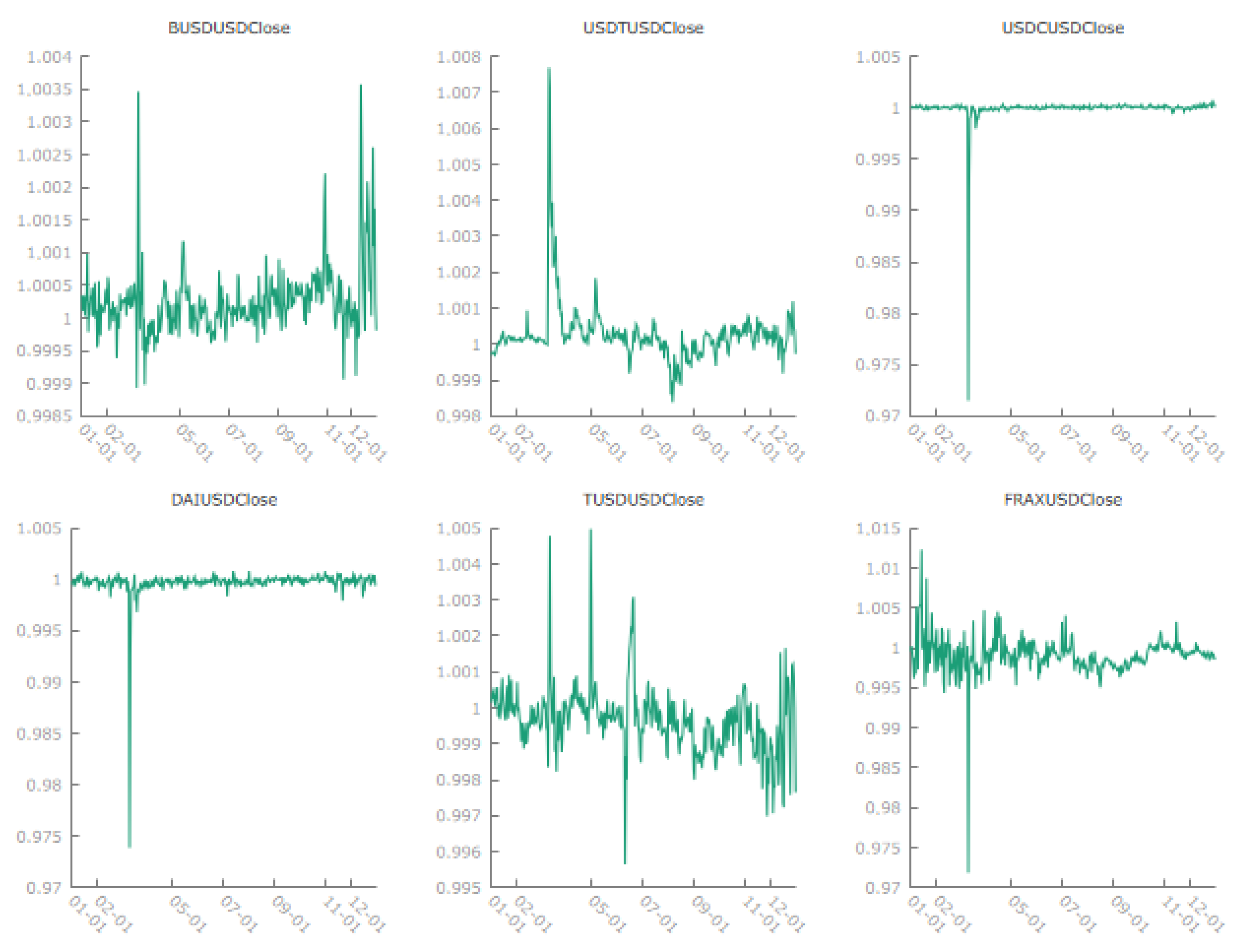
Author Contributions

Conceptualization, P.O.D. and J.C.; methodology, P.O.D. and J.C.; software, P.O.D. and J.C.; validation, J.C.; formal analysis, P.O.D.; data curation, P.O.D.; writing—original draft preparation, P.O.D. and J.C.; writing—review and editing, P.O.D. and J.C.; visualization, P.O.D. and J.C.; supervision, J.C.; project administration, P.O.D. and J.C. These authors contributed equally to this work. All authors have read and agreed to the published version of the manuscript.

Funding

This research received no external funding.

Institutional Review Board Statement

Not applicable.

Informed Consent Statement

Not applicable.

Data Availability Statement

The stablecoins and cryptocurrency data are freely available from Yahoo Finance! https://finance.yahoo.com/ (accessed on 6 January 2025).

Acknowledgments

We wish to thank Guglielmo Maria Caporale—as well as two anonymous referees for thoughtful comments that led to improve our paper. Earlier versions of this paper were presented at the International Conference on Risk and Financial Management (IOCRF, June 2025) on ‘Big Data, Artificial Intelligence, and Machine Learning in Finance’; as well as at the International Conference on Empirical Economics (ICEE, August 2025) at PennState Altoona, USA. For valuable feedback and suggestions, we are grateful to Francesco Marchionne, Petros Katsoulis, Ramona Rupeika-Apoga, and Ahmed Eltweri.

Conflicts of Interest

The authors declare no conflicts of interest.

Appendix A

Appendix A.1. Descriptive Statistics in Log Form

Table A1 presents descriptive statistics for the log-transformed volume series. The first row displays measures of central tendency and range (Mean, Median, Min, Max) with dispersion and distribution shape (Std. Dev., CV, Skewness, Kurtosis). The second row reports the 5th and 95th percentiles, the interquartile range (IQR), and the number of missing observations.
Table A1. Descriptive Statistics in Logarithmic Form.
VariableMeanMedianMinimumMaximum
l_BUSDUSDClose0.00020.0002−0.00110.0036
l_BUSDUSDVolume21.136021.309017.189023.3330
l_USDTUSDClose0.00030.0002−0.00160.0077
l_USDTUSDVolume24.037024.023023.025025.0380
l_USDCUSDClose−0.00010.0000−0.02890.0008
l_USDCUSDVolume21.956021.953020.759024.0070
l_DAIUSDClose−0.0003−0.0002−0.02650.0008
l_DAIUSDVolume18.755018.747017.641022.2590
l_TUSDUSDClose−0.0003−0.0004−0.00440.0050
l_TUSDUSDVolume19.754019.795017.007022.1590
l_FRAXUSDClose−0.0009−0.0009−0.02860.0122
l_FRAXUSDVolume16.090016.064014.518019.8060
l_BTCUSDClose10.250010.23209.718710.6960
l_BTCUSDVolume23.527023.502022.397024.7240
l_ETHUSDClose7.48547.49937.09097.7743
l_ETHUSDVolume22.658022.668021.456023.9300
l_TRXUSDClose−2.5638−2.5678−2.9561−2.2181
l_TRXUSDVolume19.177019.148018.373020.5390
VariableStd. Dev.C.V.SkewnessKurtosis
l_BUSDUSDClose0.00052.06962.440811.6270
l_BUSDUSDVolume1.29620.0613−0.71790.7096
l_USDTUSDClose0.00083.07364.769836.1510
l_USDTUSDVolume0.42400.01760.0514−0.5393
l_USDCUSDClose0.001617.0610−16.8890300.0000
l_USDCUSDVolume0.41430.01890.23571.2006
l_DAIUSDClose0.00154.9978−15.0820257.2100
l_DAIUSDVolume0.57190.03050.96663.8121
l_TUSDUSDClose0.00092.74430.87736.3895
l_TUSDUSDVolume1.51780.0768−0.3020−1.2431
l_FRAXUSDClose0.00252.7200−3.126045.4660
l_FRAXUSDVolume0.69820.04340.76712.2548
l_BTCUSDClose0.19870.01940.14700.5515
l_BTCUSDVolume0.44990.01910.0424−0.3359
l_ETHUSDClose0.12240.0164−0.14200.7382
l_ETHUSDVolume0.44430.0196−0.2076−0.2224
l_TRXUSDClose0.17620.06870.3092−0.6929
l_TRXUSDVolume0.34740.01810.97051.7886
Variable5% Perc.95% Perc.IQRMissing Obs.
l_BUSDUSDClose−0.00030.00110.00040
l_BUSDUSDVolume18.516023.03801.65990
l_USDTUSDClose−0.00060.00100.00040
l_USDTUSDVolume23.320024.73000.61230
l_USDCUSDClose−0.00030.00030.00020
l_USDCUSDVolume21.268022.61300.51540
l_DAIUSDClose−0.00100.00040.00040
l_DAIUSDVolume17.882019.60800.77290
l_TUSDUSDClose−0.00170.00090.00090
l_TUSDUSDVolume17.366021.71202.54070
l_FRAXUSDClose−0.00390.00250.00190
l_FRAXUSDVolume15.067017.14300.95860
l_BTCUSDClose9.948010.65600.15650
l_BTCUSDVolume22.773024.29300.63600
l_ETHUSDClose7.32317.71300.14480
l_ETHUSDVolume21.843023.38300.62070
l_TRXUSDClose−2.8125−2.25070.25450
l_TRXUSDVolume18.707019.79200.41090

Appendix A.2. Diagnostic Test for the VAR(1) Model on Log-Differenced Price Series

Table A2. Test statistics for the VAR(1) model on log-differenced price series.
Test TypeStatisticApprox. Distributionp-Value
Autocorrelation Test (Max order 7)
LagRao FApproximate Distributionp-Value
13.85F(81.21)0.00
22.93F(162.26)0.00
32.60F(243.27)0.00
42.37F(324.27)0.00
52.13F(405.26)0.00
62.05F(486.26)0.00
71.95F(567.25)0.00
ARCH Test (Max order 7)
LagLMDegrees of Freedom (df)p-Value
14012.8820250.00
26678.9440500.00
38704.8160750.00
410,573.8181000.00
512,163.4510,1250.00
613,666.4412,1500.00
715,158.9214,1750.00
Doornik-Hansen Test
Chi-squared(18)2436.98[p-value = 0.00]
Note: The table reports diagnostic test results for the VAR(1) model on log-differenced price series. The autocorrelation test evaluates the presence of serial correlation in the residuals up to lag 7, with the Rao F statistic, its approximate distribution, and p-values under the null hypothesis of no autocorrelation. The ARCH test checks conditional heteroskedasticity, reporting the LM statistic, degrees of freedom, and corresponding p-values for each lag. The Doornik-Hansen test assesses residual normality, with Chi-squared values and p-values shown. The small p-values across all tests indicate significant deviations from the null hypotheses.

Appendix A.3. Diagnostic Test for the VAR(1) Model on Log-Differenced Volume Series

Table A3. Test statistics for the VAR(1) model on log-differenced volume series.
Rao F/LMApprox. Dist.p-Value
Autocorrelation Test up to order 7
lag 12.79F(81.21)0.00
lag 22.37F(162.26)0.00
lag 32.12F(243.27)0.00
lag 42.13F(324.27)0.00
lag 52.14F(405.26)0.00
lag 62.07F(486.26)0.00
lag 72.10F(567.25)0.00
ARCH Test up to order 7
lag 13654.0720250.00
lag 25944.7140500.00
lag 37846.6960750.00
lag 49693.0281000.00
lag 511,561.5410,1250.00
lag 613,178.1712,1500.00
lag 714,863.3114,1750.00
Doornik-Hansen Test
χ 2 ( 18 ) = 1203.78 [0.00]
Note: The table reports diagnostic test results for the VAR(1) model on log-differenced cryptocurrency and stablecoin trading volumes. The autocorrelation test evaluates the presence of residual serial correlation up to lag 7, with an F-distribution under the null hypothesis of no autocorrelation. The ARCH test detects conditional heteroskedasticity, with increasing lag orders, and the Doornik-Hansen test checks residual normality, where χ 2 ( 18 ) indicates the test statistic follows a chi-squared distribution with 18 degrees of freedom. Across all tests, the p-values are below conventional significance thresholds, suggesting significant departures from the null hypotheses.

Note

1
See https://www.binance.com/en/square/post/1177992 (accessed on 8 January 2024).

References

  1. Acharya, V. V., Pedersen, L. H., Philippon, T., & Richardson, M. (2017). Measuring systemic risk. The Review of Financial Studies, 30(1), 2–47. [Google Scholar] [CrossRef]
  2. Ahmed, M. I., & Cassou, S. P. (2016). Does consumer confidence affect durable goods spending during bad and good economic times equally? Journal of Macroeconomics, 50, 86–97. [Google Scholar] [CrossRef]
  3. Ahmed, R., & Aldasoro, I. (2025). Stablecoins and safe asset prices (Tech. Rep.). Bank for International Settlements. [Google Scholar]
  4. Aquilina, M., Cornelli, G., Frost, J., & Gambacorta, L. (2025). Cryptocurrencies and decentralised finance: Functions and financial stability implications. BIS Papers. Bank for International Settlements. [Google Scholar]
  5. Auerbach, A. J., & Gorodnichenko, Y. (2012). Fiscal multipliers in recession and expansion. In Fiscal policy after the financial crisis (pp. 63–98). University of Chicago Press. [Google Scholar]
  6. Aujus, J. (2023). Risk analysis of busd and potential deprecation plan (Tech. Rep.). Venus IO. Available online: https://community.venus.io/t/risk-analysis-of-busd-and-potential-deprecation-plan/3353 (accessed on 1 February 2025).
  7. Bains, P., Ismail, A., Melo, F., & Sugimoto, N. (2022). Regulating the crypto ecosystem: The case of stablecoins and arrangements. International Monetary Fund. [Google Scholar]
  8. Brugnolini, L. (2018). About local projection impulse response function reliability. CEIS Research Paper 440. Tor Vergata University, Italy. [Google Scholar]
  9. Bruns, M., & Lütkepohl, H. (2022). Comparison of local projection estimators for proxy vector autoregressions. Journal of Economic Dynamics and Control, 134, 104277. [Google Scholar] [CrossRef]
  10. Cole, J. (2024). Understanding busd market cap: The rise and fall of binance usd in 2024 (Tech. Rep.). blockapps. Available online: https://blockapps.net/blog/understanding-busd-market-cap-the-rise-and-fall-of-binance-usd-in-2024/ (accessed on 1 February 2025).
  11. Dell’Erba, M. (2023). Crypto-trading platforms as exchanges. Available online: https://ssrn.com/abstract=4405361 (accessed on 1 February 2025).
  12. Dimitriadis, K. A., Koursaros, D., & Savva, C. S. (2025). The influential impacts of international dynamic spillovers in forming investor preferences: A quantile-VAR and GDCC-GARCH perspective. Applied Economics, 57(45), 7175–7195. [Google Scholar] [CrossRef]
  13. Diop, P. O. (2024). An econometric and time series analysis of the USTC depeg’s impact on the LUNA classic price crash during spring 2022’s crypto market turmoil. Commodities, 3(4), 431–459. [Google Scholar] [CrossRef]
  14. Diop, P. O., Chevallier, J., & Sanhaji, B. (2024). Collapse of Silicon Valley Bank and USDC depegging: A machine learning experiment. FinTech, 3(4), 569–590. [Google Scholar] [CrossRef]
  15. Duan, K., & Urquhart, A. (2023). The instability of stablecoins. Finance Research Letters, 52, 103573. [Google Scholar] [CrossRef]
  16. Ferreira, L. N., Miranda-Agrippino, S., & Ricco, G. (2025). Bayesian local projections. Review of Economics and Statistics, 107(5), 1424–1438. [Google Scholar] [CrossRef]
  17. Galati, L., & Capalbo, F. (2024). Silicon Valley Bank bankruptcy and stablecoins stability. International Review of Financial Analysis, 91, 103001. [Google Scholar] [CrossRef]
  18. Giudici, P., Leach, T., & Pagnottoni, P. (2022). Libra or Librae? Basket based stablecoins to mitigate foreign exchange volatility spillovers. Finance Research Letters, 44, 102054. [Google Scholar] [CrossRef]
  19. Goforth, C. (2023). The securities and exchange commission and cryptoassets: A study in irony. Albany Law Review, 87(1), 55. [Google Scholar]
  20. Gonçalves, S., Herrera, A. M., Kilian, L., & Pesavento, E. (2024). State-dependent local projections. Journal of Econometrics, 244(2), 105702. [Google Scholar] [CrossRef]
  21. Gushterov, K. (2023). Binance and Changpeng Zhao face legal hurdles following supreme court decision (Tech. Rep.). Crypto DNES. Available online: https://cryptodnes.bg/en/binance-and-changpeng-zhao-face-legal-hurdles-following-supreme-court-decision/ (accessed on 1 February 2025).
  22. Herbst, E. P., & Johannsen, B. K. (2024). Bias in local projections. Journal of Econometrics, 240(1), 105655. [Google Scholar] [CrossRef]
  23. Inoue, A., Rossi, B., & Wang, Y. (2024). Local projections in unstable environments. Journal of Econometrics, 244(2), 105726. [Google Scholar] [CrossRef]
  24. Jordà, Ò. (2005). Estimation and inference of impulse responses by local projections. American Economic Review, 95(1), 161–182. [Google Scholar] [CrossRef]
  25. Li, D., Plagborg-Møller, M., & Wolf, C. K. (2024). Local projections vs. vars: Lessons from thousands of dgps. Journal of Econometrics, 244(2), 105722. [Google Scholar] [CrossRef]
  26. Lunde, V. (2023). The sec sharpens its knives (Tech. Rep.). K33 Research. Available online: https://k33.com/research/archive/articles/the-sec-sharpens-its-knives (accessed on 1 February 2025).
  27. Łęt, B., Sobański, K., Świder, W., & Włosik, K. (2023). What drives the popularity of stablecoins? Measuring the frequency dynamics of connectedness between volatile and stable cryptocurrencies. Technological Forecasting and Social Change, 189, 122318. [Google Scholar] [CrossRef]
  28. Montiel Olea, J. L., & Plagborg-Møller, M. (2021). Local projection inference is simpler and more robust than you think. Econometrica, 89(4), 1789–1823. [Google Scholar] [CrossRef]
  29. Palazzi, R. B., Schich, S., & de Genaro, A. (2025). Stablecoins as anchors? Unraveling information flow dynamics between pegged and unpegged crypto-assets and fiat currencies. Journal of International Financial Markets, Institutions and Money, 99, 102108. [Google Scholar] [CrossRef]
  30. Qiǎn, Q. (2023). Does the sec want to force binance to death? zhao changpeng is in constant trouble, here’s a quick look at the whole process (Tech. Rep.). Binance Square. Available online: https://www.binance.com/en/square/post/1170330 (accessed on 1 February 2025).
  31. Skinner, C. P. (2023). Coins, cross-border payments, and anti-money laundering law. Harvard Journal on Legislation, 60, 285. [Google Scholar]
  32. Trautman, L. J., Elzweig, B., & Newman, N. F. (2024). The SEC, fraud, and crypto currencies. Missouri Law Review, 90(2), 425–476. [Google Scholar]
  33. Wilmarth, A. E. (2023). We must protect investors and our banking system from the crypto industry. Available online: https://ssrn.com/abstract=4360175 (accessed on 1 February 2025).
  34. Zijing, T. (2023). Busd is about to be delisted. What impact will it have on binance and the market? (Tech. Rep.). Binance Square. Available online: https://www.binance.com/en-IN/square/post/1074665 (accessed on 1 February 2025).
Figure 1. Data for stablecoins. Note: BUSDUSDClose stands for the Binance’s BUSD Closing Price, USDTUSDClose for the Tether’s USDT Closing Price, USDCUSDClose for the Circle’s USDC Closing Price, DAIUSDClose for the DAI Closing Price, TUSDUSDClose for the True USD Closing Price, and FRAXUSDClose for the FRAX Closing Price in daily frequency from 1 January to 31 December 2023.
Econometrics 14 00006 g001
Figure 2. Data for cryptocurrencies. Note: BTCUSDClose stands for the Bitcoin’s Closing Price, ETHUSDClose for the Ethereum’s Closing Price, and TRXUSDClose for the TRON Closing price in daily frequency from 1 January to 31 December 2023.
Econometrics 14 00006 g002
Figure 3. Data for volumes. Note: BUSDUSDVolume stands for the Binance’s BUSD Volumes Exchanged, USDTUSDVolume for the Tether’s USDT Volumes Exchanged, USDCUSDVolume for the Circle’s USDC Volumes Exchanged, DAIUSDVolume for the DAI Volumes Exchanged, TUSDUSDVolume for the True USD Volumes Exchanged, and FRAXUSDVolume for the FRAX Volumes Exchanged, BTCUSDVolume stands for the Bitcoin’s Volumes Exchanged, ETHUSDVolume for the Ethereum’s Volumes Exchanged, and TRXUSDVolume for the TRON Volumes Exchanged in daily frequency from 1 January to 31 December 2023.
Econometrics 14 00006 g003
Figure 4. Local projection on Prices: Negative Reactions from BUSD Shock.
Econometrics 14 00006 g004
Figure 5. Local projection on Prices: Positive Reactions from BUSD Shock.
Econometrics 14 00006 g005
Figure 6. Local projection on Prices: No Visible Reactions from BUSD Shock.
Econometrics 14 00006 g006
Figure 7. Net migration of trading volume from BUSD to USDT/USDC (and to DAI/FRAX/TUSD). Note: USDT is Tether’s USDT Closing Price; USDC is Circle’s USDC Closing Price; FDUSD is the FRAX Closing Price; DAI is the DAI Closing Price; and TUSD is the True USD Closing Price.
Econometrics 14 00006 g007
Figure 8. Local projection on Volumes: Positive Reactions from BUSD Shock.
Econometrics 14 00006 g008
Figure 9. Local projection on Volumes: Negative Reactions from BUSD Shock.
Econometrics 14 00006 g009
Figure 10. Local projection on Volumes: No Visible Reactions from BUSD Shock.
Econometrics 14 00006 g010
Figure 11. Nonlinear local projection: Dummy variable from BUSD Volume.
Econometrics 14 00006 g011
Figure 12. Nonlinear local projection: USDT Reactions from BUSD Price Shock.
Econometrics 14 00006 g012
Figure 13. Nonlinear local projection: USDC Reactions from BUSD Price Shock.
Econometrics 14 00006 g013
Figure 14. Nonlinear local projection: DAI Reactions from BUSD Price Shock.
Econometrics 14 00006 g014
Figure 15. Nonlinear local projection: TUSD Reactions from BUSD Price Shock.
Econometrics 14 00006 g015
Figure 16. Nonlinear local projection: FRAX Reactions from BUSD Price Shock.
Econometrics 14 00006 g016
Figure 17. Nonlinear local projection: BTC Reactions from BUSD Price Shock.
Econometrics 14 00006 g017
Figure 18. Nonlinear local projection: ETH Reactions from BUSD Price Shock.
Econometrics 14 00006 g018
Figure 19. Nonlinear local projection: TRX Reactions from BUSD Price Shock.
Econometrics 14 00006 g019
Figure 20. Nonlinear local projection: USDT Reactions from BUSD Volume Shock.
Econometrics 14 00006 g020
Figure 21. Nonlinear local projection: USDC Reactions from BUSD Volume Shock.
Econometrics 14 00006 g021
Figure 22. Nonlinear local projection: DAI Reactions from BUSD Volume Shock.
Econometrics 14 00006 g022
Figure 23. Nonlinear local projection: TUSD Reactions from BUSD Volume Shock.
Econometrics 14 00006 g023
Figure 24. Nonlinear local projection: FRAX Reactions from BUSD Volume Shock.
Econometrics 14 00006 g024
Figure 25. Nonlinear local projection: BTC Reactions from BUSD Volume Shock.
Econometrics 14 00006 g025
Figure 26. Nonlinear local projection: ETH Reactions from BUSD Volume Shock.
Econometrics 14 00006 g026
Figure 27. Nonlinear local projection: TRX Reactions from BUSD Volume Shock.
Econometrics 14 00006 g027
Figure 28. Markov-switching VAR: Regimes identification for Price series. Note: The dataset comprises stablecoin series—BUSDUSDClose (Binance), USDTUSDClose (Tether), USDCUSDClose (Circle), DAIUSDClose (DAI), TUSDUSDClose (True USD), and FRAXUSDClose (FRAX)—and cryptocurrency series—BTCUSDClose (Bitcoin), ETHUSDClose (Ethereum), and TRXUSDClose (TRON) based on daily data from 1 January to 31 December 2023.
Econometrics 14 00006 g028
Figure 29. Markov-switching VAR: Regimes identification for Volume series (in log form). Note: The dataset comprises stablecoin volume series—BUSDUSDVolume (Binance’s BUSD Volumes Exchanged), USDTUSDVolume (Tether’s USDT Volumes Exchanged), USDCUSDVolume (Circle’s USDC Volumes Exchanged), DAIUSDVolume (DAI Volumes Exchanged), TUSDUSDVolume (True USD Volumes Exchanged), and FRAXUSDVolume (FRAX Volumes Exchanged)—and cryptocurrency volume series—BTCUSDVolume (Bitcoin’s Volumes Exchanged), ETHUSDVolume (Ethereum’s Volumes Exchanged), and TRXUSDVolume (TRON’s Volumes Exchanged), based on daily data from 1 January to 31 December 2023, presented in logarithmic form.
Econometrics 14 00006 g029aEconometrics 14 00006 g029b
Table 1. Descriptive Statistics.
VariableMeanMedianMinimumMaximum
BUSDUSDClose1.00021.00020.99891.0036
BUSDUSDVolume2874.80001796.200029.181013,601.0000
USDTUSDClose1.00031.00020.99841.0077
USDTUSDVolume30,076.000027,118.00009989.900074,778.0000
USDCUSDClose0.99991.00000.97151.0008
USDCUSDVolume3753.60003419.80001036.800026,682.0000
DAIUSDClose0.99970.99980.97391.0008
DAIUSDVolume174.9500138.620045.84804642.5000
TUSDUSDClose0.99970.99970.99561.0050
TUSDUSDVolume887.3000395.380024.32004203.1000
FRAXUSDClose0.99910.99910.97191.0123
FRAXUSDVolume13.46709.47272.0185399.5800
BTCUSDClose28,859.000027,767.000016,625.000044,167.0000
BTCUSDVolume18,251.000016,101.00005331.200054,622.0000
ETHUSDClose1795.20001806.80001201.00002378.7000
ETHUSDVolume7611.20006990.30002081.600024,710.0000
TRXUSDClose0.07820.07670.05200.1088
TRXUSDVolume227.9800206.860095.3470832.0800
VariableStd. Dev.CVSkewnessKurtosis
BUSDUSDClose0.00050.00052.446711.6670
BUSDUSDVolume3104.00001.07971.52611.3914
USDTUSDClose0.00080.00084.788336.3670
USDTUSDVolume13,086.00000.43510.98280.7240
USDCUSDClose0.00160.0016−16.8490298.8500
USDCUSDVolume1926.00000.51315.068853.8120
DAIUSDClose0.00150.0015−15.0100255.4000
DAIUSDVolume262.96001.503113.8900228.0200
TUSDUSDClose0.00090.00090.88806.4262
TUSDUSDVolume940.67001.06011.07190.3669
FRAXUSDClose0.00240.0024−2.988543.8810
FRAXUSDVolume23.62301.754112.6490196.2300
BTCUSDClose5900.00000.20440.82190.6612
BTCUSDVolume8529.50000.46741.19121.6516
ETHUSDClose219.26000.12210.32530.4802
ETHUSDVolume3342.50000.43920.97951.5092
TRXUSDClose0.01420.18110.6083−0.5826
TRXUSDVolume100.22000.43962.754510.4950
Variable5% Perc.95% Perc.IQRMissing Obs.
BUSDUSDClose0.99971.00110.00040
BUSDUSDVolume116.070010,124.00002826.10000
USDTUSDClose0.99941.00100.00040
USDTUSDVolume13,421.000054,983.000017,117.00000
USDCUSDClose0.99971.00030.00020
USDCUSDVolume1724.10006619.20001781.50000
DAIUSDClose0.99901.00040.00040
DAIUSDVolume58.3270327.9200107.23000
TUSDUSDClose0.99831.00090.00090
TUSDUSDVolume34.81702689.00001486.70000
FRAXUSDClose0.99611.00250.00190
FRAXUSDVolume3.495527.88009.48180
BTCUSDClose20,909.000042,445.00004391.80000
BTCUSDVolume7762.300035,498.000010,767.00000
ETHUSDClose1514.90002237.2000255.11000
ETHUSDVolume3064.200014,288.00004330.50000
TRXUSDClose0.06010.10530.01930
TRXUSDVolume133.1700394.210085.39300
Note: All volume figures represent millions of units (original values divided by 1,000,000).
Table 2. Log-differenced Price Series: Results for VAR System with Maximum Lag Order of 14.
LagsLog-Likelihoodp(LR)AICBICHQC
115,128.07−85.93−84.94 *−85.54
215,283.880.00−86.36−84.47−85.61 *
315,372.230.00−86.40 *−83.62−85.30
415,451.300.00−86.39−82.72−84.93
515,528.600.00−86.37−81.81−84.55
615,595.250.00−86.29−80.83−84.12
715,672.630.00−86.27−79.92−83.74
815,747.800.00−86.23−78.99−83.35
915,816.700.00−86.16−78.03−82.93
1015,883.340.00−86.08−77.05−82.49
1115,961.550.00−86.07−76.15−82.12
1216,023.800.00−85.96−75.15−81.65
1316,098.460.00−85.92−74.22−81.26
1416,171.440.00−85.88−73.28−80.86
Note: Asterisks indicate the best (i.e., lowest) values of the following information criteria, AIC = Akaike criterion, BIC = Schwartz Bayesian criterion and HQC = Hannan–Quinn criterion.
Table 3. Log-differenced Volumes: Results for VAR System with Maximum Lag Order of 14.
LagsLog-Likelihoodp(LR)AICBICHQC
1420.14−1.89−0.89 *−1.49 *
2536.650.00−2.09−0.20−1.34
3621.390.00−2.110.67−1.01
4690.180.00−2.041.63−0.58
5786.480.00−2.132.43−0.31
6873.720.00−2.163.290.01
7966.810.00−2.23 *4.120.29
81044.310.00−2.215.030.67
91115.240.00−2.165.981.08
101172.630.01−2.027.011.57
111260.680.00−2.067.861.89
121304.430.29−1.858.972.46
131377.350.00−1.809.902.86
141456.980.00−1.7910.803.22
Note: Asterisks indicate the best (i.e., lowest) values of the following information criteria, AIC = Akaike criterion, BIC = Schwartz Bayesian criterion and HQC = Hannan–Quinn criterion.
Table 4. VAR(1) System for Log-differenced Price Series.
BUSDUSDTUSDCDAITUSDFRAXBTCETHTRX
const0.000.00−0.00−0.000.000.000.00 *0.000.00
(0.74)(0.71)(0.80)(0.91)(0.91)(0.89)(0.04)(0.16)(0.07)
BUSD(−1)−0.09−0.22 ***1.45 ***1.40 ***0.26 **1.60 ***3.942.570.53
(0.13)(0.00)(0.00)(0.00)(0.01)(0.00)(0.19)(0.43)(0.86)
USDT(−1)−0.070.08−1.79 ***−1.77 ***0.00−1.93 ***1.370.793.37
(0.30)(0.21)(0.00)(0.00)(0.98)(0.00)(0.69)(0.83)(0.30)
USDC(−1)−0.07 *−0.26 ***0.020.39 **−0.23 **0.16−0.260.14−0.68
(0.09)(0.00)(0.90)(0.01)(0.00)(0.54)(0.91)(0.96)(0.76)
DAI(−1)−0.050.22 ***−0.54 **−0.93 ***0.11−0.310.86−0.320.33
(0.36)(0.00)(0.00)(0.00)(0.24)(0.29)(0.75)(0.91)(0.90)
TUSD(−1)−0.06 *−0.050.30 **0.28 **−0.28 ***0.44 **−0.930.001.80
(0.06)(0.11)(0.01)(0.01)(0.00)(0.02)(0.58)(1.00)(0.27)
FRAX(−1)−0.000.02−0.09 **−0.08 *−0.01−0.50 ***−0.42−0.41−0.44
(0.70)(0.15)(0.03)(0.05)(0.68)(0.00)(0.48)(0.52)(0.44)
BTC(−1)−0.00 **−0.000.00−0.00−0.00−0.010.110.10−0.03
(0.04)(0.32)(0.87)(0.64)(0.39)(0.51)(0.25)(0.34)(0.75)
ETH(−1)−0.000.000.000.00−0.00−0.01−0.07−0.17 *−0.00
(0.81)(0.35)(0.86)(0.93)(0.35)(0.60)(0.47)(0.09)(0.98)
TRX(−1)0.00−0.00 ***0.01 **0.01 **0.000.01−0.06−0.01−0.09
(0.34)(0.01)(0.02)(0.04)(0.90)(0.54)(0.36)(0.85)(0.16)
Note: p-values in parentheses. *** p < 0.01, ** p < 0.05, * p < 0.1. The notation (−1) refers to the lag 1 value in the VAR(p) model estimation. Observations: 3 January 2023–31 December 2023 (T = 363). Log likelihood = 15,666.60, AIC = −85.82, BIC = −84.86.
Table 5. VAR(1) System for Log-differenced Volume Series.
BUSDUSDTUSDCDAITUSDFRAXBTCETHTRX
const−0.010.010.010.010.010.000.010.010.00
(0.52)(0.72)(0.72)(0.76)(0.66)(0.99)(0.78)(0.75)(0.92)
BUSD(−1)0.070.24 **0.27 **0.26 *0.32 **0.180.32 **0.28 **0.03
(0.45)(0.02)(0.02)(0.07)(0.03)(0.41)(0.01)(0.03)(0.80)
USDT(−1)−0.21−0.57 ***−0.38 **−0.32 *−0.33 *−0.22−0.39 **−0.32 **−0.16
(0.11)(0.00)(0.01)(0.08)(0.08)(0.43)(0.02)(0.05)(0.24)
USDC(−1)−0.30 ***−0.19−0.52 ***0.04−0.22−0.19−0.28 **−0.210.16
(0.01)(0.13)(0.00)(0.80)(0.19)(0.44)(0.05)(0.14)(0.18)
DAI(−1)0.020.000.06−0.34 ***0.010.050.020.040.02
(0.67)(0.98)(0.36)(0.00)(0.86)(0.68)(0.73)(0.60)(0.71)
TUSD(−1)0.030.080.070.010.080.28 **0.110.100.03
(0.67)(0.24)(0.36)(0.88)(0.38)(0.03)(0.14)(0.17)(0.69)
FRAX(−1)0.040.06 **0.10 ***0.08 **0.05−0.35 ***0.10 ***0.08 **−0.01
(0.17)(0.04)(0.00)(0.05)(0.28)(0.00)(0.01)(0.03)(0.85)
BTC(−1)0.170.180.220.09−0.16−0.17−0.010.150.02
(0.16)(0.17)(0.13)(0.61)(0.38)(0.53)(0.96)(0.33)(0.90)
ETH(−1)0.060.100.140.140.190.320.07−0.25 *−0.01
(0.63)(0.42)(0.32)(0.39)(0.28)(0.20)(0.64)(0.09)(0.95)
TRX(−1)−0.13 **−0.12 *−0.13 *−0.13−0.010.07−0.15 **−0.12−0.26 ***
(0.02)(0.07)(0.07)(0.13)(0.93)(0.58)(0.04)(0.11)(0.00)
Note: p-values in parentheses. *** p < 0.01, ** p < 0.05, * p < 0.1. The notation (−1) refers to the lag 1 value in the VAR(p) model estimation. The suffix _VOL indicates the volumes exchanged for each asset, as opposed to closing prices. Observations: 3 January 2023–31 December 2023 (T = 363). Log likelihood = 407.73, AIC = −1.75, BIC = −0.79.
Table 6. MS-VAR estimates for the Price series.
Number of Iterations19
Log-Likelihood2372.17
Initial state probabilities
State 10.00
State 21.00
   
Transition matrix
to State 1to State 2
from State 10.910.09
from State 20.020.98
   
Response parameters
Gaussian distribution
InterceptStandard deviation
State 11.000.00
State 21.000.00
Note: The table presents estimated parameters from a two-regime Markov-switching VAR model, using daily closing prices of cryptocurrencies and stablecoins from 2023. It includes the number of iterations and log-likelihood, indicating model convergence and fit. Initial state probabilities show the likelihood of starting in each regime, while the transition matrix details probabilities for staying in or moving between regimes. High diagonal probabilities suggest strong persistence in specific regimes. Response parameters outline characteristics unique to each regime, with the intercept reflecting the mean level and standard deviation representing dispersion for the error term. These estimates offer insight into the dynamic, regime-dependent behavior of the price series.
Table 7. MS-VAR estimates for the Volume series (in log form).
Number of Iterations25
Log-Likelihood−128.51
Initial state probabilities
State 11.00
State 20.00
   
Transition matrix
to State 1to State 2
from State 10.9950.005
from State 20.0001.000
   
Response parameters
Gaussian distribution
InterceptStandard deviation
State 19.560.29
State 28.680.42
Note: The table presents estimated parameters from a two-regime Markov-switching VAR model for cryptocurrency and stablecoin volume series (in logarithmic form), using daily volume data from 2023. The number of iterations and log-likelihood indicate model convergence and fit. Initial state probabilities highlight the likelihood of starting in each regime, while the transition matrix shows the probabilities of remaining in or transitioning between regimes, with strong persistence in State 1. Response parameters outline characteristics for each regime, with the intercept reflecting the mean log-volume level and the standard deviation indicating the dispersion of errors. These results provide insight into the regime-dependent dynamics of trading volumes.
Disclaimer/Publisher’s Note: The statements, opinions and data contained in all publications are solely those of the individual author(s) and contributor(s) and not of MDPI and/or the editor(s). MDPI and/or the editor(s) disclaim responsibility for any injury to people or property resulting from any ideas, methods, instructions or products referred to in the content.