Locationally Varying Production Technology and Productivity: The Case of Norwegian Farming

Abstract

In this study, we leverage geographical coordinates and firm-level panel data to uncover variations in production across different locations. Our approach involves using a semiparametric proxy variable regression estimator, which allows us to define and estimate a customized production function for each firm and its corresponding location. By employing kernel methods, we estimate the nonparametric functions that determine the model’s parameters based on latitude and longitude. Furthermore, our model incorporates productivity components that consider various factors that influence production. Unlike spatially autoregressive-type production functions that assume a uniform technology across all locations, our approach estimates technology and productivity at both the firm and location levels, taking into account their specific characteristics. To handle endogenous regressors, we incorporate a proxy variable identification technique, distinguishing our method from geographically weighted semiparametric regressions. To investigate the heterogeneity in production technology and productivity among Norwegian grain farmers, we apply our model to a sample of farms using panel data spanning from 2001 to 2020. Through this analysis, we provide empirical evidence of regional variations in both technology and productivity among Norwegian grain farmers. Finally, we discuss the suitability of our approach for addressing the heterogeneity in this industry.

1. Introduction

Some of the more common assumptions in the econometric estimation of production function are related to the independence and homogeneity of the production units. That is, the production technology is assumed to be homogeneous, and possible externalities (spillover effects) are ruled out. However, in the context of farming, where production is primarily a biological process, this may not be the case. For this reason, the analysis of agricultural production should typically be more nuanced and account for differences in technology that satisfy the environmental and social conditions within which farms operate. Farming is also a somewhat unique industry in terms of the extent to which it is possible to get a handle on the natural characteristics of land that determine natural advantages, such as soil type and moisture, plant fertility, the potential for crop diseases and weed infestations, the gradient of the land, the climate, etc. (e.g., Holmes and Lee 2012; Postiglione et al. 2022). As an example, farmers usually choose to grow varieties that are best suited to the environmental and climatic conditions in which the farms operate.

Heterogeneity also arises because of the way the economic system works. Some farms have advantages because they are located close to markets (which implies lower transportation costs, either to the local market or to food processing) and/or have easier access to labor, human capital, and expert advisors. It can also be due to differences between farms and regions in terms of government restrictions, support systems, etc. (e.g., Capello 2009). All of the above-mentioned aspects require agricultural production analyses (and their corresponding production functions) to account for heterogeneity. Further, existing studies in the literature support the idea that producers do not even operate on the basis of a single homogeneous technology (e.g., Dosi and Nelson 2010; Eberhardt and Teal 2013; Just and Pope 2001; Mundlak 2001; Syverson 2011).

For this reason, many existing studies control for the possibility of heterogeneous technology. One way is to use classification (e.g., firm location) or cluster analysis (statistical classification based on some observed variables) to estimate different production functions for each class or group (e.g., Álvarez et al. 2008). This “observed” classification to deal with heterogeneity among firms is challenging. The identification of heterogeneity requires comprehensive spatial modeling of soil as well as agronomic and climatic properties, including changes through time. This identification then requires processing of large quantities of data acquired at a very fine spatial resolution. In practice, it is hard or even sometimes impossible to gain access to all these data for “observed” classification, and researchers often need to rely on only a few control variables. Therefore, a drawback of this “observed” classification approach of splitting a sample of observations (firms) is that differences in technology will typically be the result of both observed and unobserved heterogeneity (Billé et al. 2018).

Modeling unobserved heterogeneity can be accomplished via finite mixture/latent class methods, nonparametric methods, and fixed/random effects panel data analyses (e.g., Greene 2005; Kumbhakar and Tsionas 2010; O’Donnell and Griffiths 2006; Orea and Kumbhakar 2004; Saint-Cyr et al. 2019; Sauer and Paul 2013). However, this approach cannot strictly identify which technology is used by which firm.

The extension beyond the cross-sectional input use and outcome of the production function analysis framework so far in the agricultural production economics literature has mostly been on the temporal dimension (i.e., the time series aspects of the analysis) and firm/farm heterogeneity (as reviewed briefly before). In other words, in the literature on agricultural production economics, the temporal analysis of economic development and firm heterogeneity has received the most attention, and the variable “space” has typically received less attention and is often neglected (e.g., Capello 2009; Eberhardt and Teal 2013; Isard 1954). This is clearly pointed out by Just and Pope (2001) (p. 651): 1

“Spatial dimensions of input groupings may be particularly important in agriculture because the inputs must be tailored to the heterogeneity of firm resources, which differ substantially by climate and land quality (location).”

There are several commonly given reasons for this, including the need to simplify the treatment and models (Capello 2009), data limitations (Just and Pope 2001), and lack of access to computer power for estimation.

There are two distinguishable spatial effects that can be identified: spatial dependency and spatial heterogeneity. Spatial dependency, which involves analyzing the transfer of effects between locations, is a specific case of cross-sectional dependence. It arises from the correlation or covariance structure between random variables at different locations, determined by their relative positions (distances) in geographic space. Analyzing spatial dependency often requires specialized techniques, such as spatial lag models (SLM), spatial autoregressive models (SAR), spatial cross-regressive models (SLX), or spatial error models (SEM) (Anselin 2010). Although these approaches consider spatial relationships in terms of output/input quantities at the local level, they assume that the production technology remains consistent for all firms or farms. In other words, these methods do not account for the spatial heterogeneity in production technology across different locations. Among others, the concept of spatial dependency in agricultural production economics has been used to analyze crop diversification (e.g., Holmes and Lee 2012), drivers of technology adoption (e.g., Läpple and Kelley 2015; Läpple et al. 2017; Schmidtner et al. 2012), land rental intentions (e.g., Skevas et al. 2018), pesticide use (e.g., Aida 2018), variation in farmland values (e.g., Wang 2018), and analysis of policy intervention (e.g., Storm et al. 2015).

Spatial heterogeneity is a special case of unobserved heterogeneity. This framework accounts for the absence of stability and implies estimating parameters that vary over space. In contrast to spatial dependency, this framework does not always require a separate set of methods. Spatial heterogeneity provides the basis for the specification or structure of heterogeneity in a spatial model (Anselin 2010). In the literature, we find several studies that have used locally weighted regression (LWR) (McMillen and Redfearn 2010) or geographically weighted semiparametric regressions (GWR) (Brunsdon et al. 1996). Past applications within agricultural production economics include analysis of spatial regimes in olive farm technology in Italy (Billé et al. 2018), factors affecting fertilizer use efficiency in China (Bai et al. 2021), and space–time patterns of regional industrial resilience among Italian wine producers (Canello and Vidoli 2020).

In this study, we employ the spatial heterogeneity approach proposed by Malikov et al. (2022) to examine the productivity of the Norwegian grain farming sector. This approach entails estimating a production function that is specific to each firm and location, using a semiparametric proxy variable regression estimator. The parameters of the model are nonparametric functions derived from the geographical coordinates (latitude and longitude) of the firms, which are estimated using kernel methods. The model incorporates productivity components to account for the factors that influence productivity. This methodology enables us to estimate technologies that are specific to each firm and location, as well as productivity measures that are specific to each firm and location. Unlike, for example, the GWR approach mentioned earlier, our method can handle endogenous regressors through a proxy variable estimation technique. We applied this model to analyze the productivity of Norwegian grain farmers using panel data at the farm level, covering the period from 2001 to 2020. The significance of our study lies in evaluating the effectiveness of utilizing the aforementioned approach, which incorporates location- and firm-specific semiparametric production functions with longitude/latitude coordinates as a means to capture spatial variations among firms/farms and locations when analyzing production technology and productivity within the farming industries.

2. Locational Heterogeneity in Production

Consider firm i ($i=1,\dots ,n$) during time period t ($t=1,\dots ,T$). In line with the existing productivity literature (e.g., see Ackerberg et al. 2015; Blundell and Bond 2000; Collard-Wexler and De Loecker 2015; Doraszelski and Jaumandreu 2013; Konings and Vanormelingen 2015; Levinsohn and Petrin 2003; Olley and Pakes 1996), we make the assumption that the firm employs physical capital $K_{it}$, labor $L_{it}$, land $N_{it}$, and an intermediate input such as materials $M_{it}$ to generate a single output $Y_{it}$ using Cobb–Douglas production technology, which incorporates unobserved Hicks-neutral productivity:

$$Y_{it}=A_0\left(s_i\right)K_{it}^{{\alpha }_K\left(s_i\right)}{L}_{it}^{{\alpha }_L\left(s_i\right)}{N}_{it}^{{\alpha }_N\left(s_i\right)}{M}_{it}^{{\alpha }_M\left(s_i\right)}\exp \left\{{\omega }_{it}+{\eta }_{it}\right\},$$

(1)

where $s_i={(s_{1i},s_{2i})}^{\prime }$ represents the fixed location of firm i, and $s_{1i}$ and $s_{2i}$ are the latitude and longitude coordinates of the firm’s location. $A_0\left(s_i\right)$ is a firm- and location-specific scalar constant; ${({\alpha }_K\left(s_i\right),{\alpha }_L\left(s_i\right),{\alpha }_N\left(s_i\right),{\alpha }_M\left(s_i\right))}^{\prime }$ are firm- and location-specific input elasticities; and ${\omega }_{it}$ is the firm’s persistent productivity, which is known to the firm at time t but unknown to others and which, as we discuss later, follows an evolution process that is also specific to firm location. By incorporating location-specific heterogeneity in the elasticities of inputs and persistent productivity, we account for the effects of technology spillovers and agglomeration economies, which are influenced by local neighborhood effects. Additionally, following the literature, we introduce ${\eta }_{it}$ as a random, independent, and identically distributed (i.i.d.) productivity shock. We assume that ${\eta }_{it}$ is a random i.i.d. productivity shock such that $E\left[{\eta }_{it}\right|{\mathcal{I}}_{it}]=E\left[{\eta }_{it}\right]=0$, where ${\mathcal{I}}_{it}$ is the information set available to firm i for making period t production decisions. Thus, the expectation of exponential random shock ${\eta }_{it}$ is $\theta \equiv \mathbb{E}\left[\exp \left\{{\eta }_{it}\right\}\right|{\mathcal{I}}_{it}]=\mathbb{E}\left[\exp \left\{{\eta }_{it}\right\}\right]$, which is a constant. As such, $\theta$ does not play an important role; it is a nuisance parameter. Since the production shock is unknown due to the presence of $\eta$, the conventional procedure is to eliminate it by assuming the expected profit maximization (shown later in Equation (4)), which involves the expectation of $\mathbb{E}\left[\exp \left\{{\eta }_{it}\right\}\right]$.

Following the productivity literature (e.g., Gandhi et al. 2020; Malikov and Lien 2021; Malikov and Zhao 2021; Malikov et al. 2020, 2022), physical capital $K_{it}$, labor $L_{it}$, and land $N_{it}$ are subject to adjustment frictions (e.g., time-to-install, hiring/training costs). The firm optimizes these inputs dynamically at time $t-1$, making them predetermined (quasi-fixed) state variables at time t. Materials $M_{it}$ are determined statically by the firm at time t, making it a freely varying (flexible) input. Thus, $K_{it}$, $L_{it}$, and $N_{it}$ are state variables that follow the dynamic laws of motion, viz.,

$$K_{it}=I_{it-1}+(1-\delta )K_{it-1},L_{it}=H_{it-1}+L_{it-1},\mathrm{and}{N}_{it}=N_{it-1}+\Delta N_{it-1},$$

(2)

where $I_{it}$, $H_{it}$, $\delta$, and $\Delta N_{it-1}$ are gross investment, net hiring, the depreciation rate, and net change in land use, respectively.

Building on insights from the proxy variable literature (e.g., De Loecker 2013; Doraszelski and Jaumandreu 2013; Gandhi et al. 2020; Malikov and Lien 2021; Malikov and Zhao 2021; Malikov et al. 2020, 2022), we utilize a first-order Markov process to capture the dynamics of firm productivity ${\omega }_{it}$. The evolution of ${\omega }_{it}$, representing the productivity of the firm, is shaped by a range of factors, denoted as X, which are specific to the particular empirical context. Thus, ${\omega }_{it}$ is modeled according to a location-varying controlled first-order Markov process:

$${\omega }_{it}=h_{|s_i}\left({\omega }_{it-1},X_{it-1}\right)+{\zeta }_{it},$$

(3)

where $h_{|s_i}(·)$ is the conditional mean function of ${\omega }_{it}$, which varies across space, and ${\zeta }_{it}$ is a random innovation in persistent productivity that is unanticipated by the firm at period $t-1$: $E\left[{\zeta }_{it}|{\mathcal{I}}_{it-1}\right]=E\left[{\zeta }_{it}|{\omega }_{it-1},X_{it-1}\right]=E\left[{\zeta }_{it}\right]=0$.

The relationship between ${\omega }_{it}$ and the control variables $X_{it}$ incorporates a lagged structure in the evolutionary process, as defined by Equation (3). This acknowledgment implicitly recognizes that activities aimed at enhancing productivity and learning incur costs and may require time to produce tangible results. Additionally, in $\mathbb{E}\left[{\zeta }_{it}\right|{\mathcal{I}}_{it-1}]=0$, we assume that, given the adjustment costs, firms do not experience changes in their productivity-related investments in light of productivity innovation. That is, a firm cannot anticipate innovation ${\zeta }_{it}$ and chooses the level of $X_{it-1}$ in period $t-1$ based on its knowledge of the contemporaneous productivity ${\omega }_{it-1}$. These structural timing assumptions about ${\zeta }_{it}$ are common in models with controlled productivity processes (e.g., Van Biesebroeck 2005; Doraszelski and Jaumandreu 2013, 2018; De Loecker 2013; Malikov et al. 2020, 2022) and are needed to identify productivity-enhancing learning effects.

Given the intermediate input $M_{it}$ is freely varying and thus affects profits only in the current period, the risk-neutral firm chooses its optimal level of freely varying input $M_{it}$ via solving the (static) restricted expected profit-maximization problem subject to the already optimal dynamic choice of quasi-fixed inputs:

$$\begin{array}{c}\hfill \underset{M_{it}}{\max }{P}_t^Y{A}_0\left(s_i\right)K_{it}^{{\alpha }_K\left(s_i\right)}{L}_{it}^{{\alpha }_L\left(s_i\right)}{N}_{it}^{{\alpha }_N\left(s_i\right)}{M}_{it}^{{\alpha }_M\left(s_i\right)}\exp \left\{{\omega }_{it}\right\}\theta -P_t^M{M}_{it},\end{array}$$

(4)

where $P_t^Y$ and $P_t^M$ are the output and material prices, respectively, both of which are competitively determined, and $\theta \equiv \mathbb{E}\left[\exp \left\{{\eta }_{it}\right\}\right|{\mathcal{I}}_{it}]$. The firm’s conditional demand for $M_{it}$ is derived by applying the first-order condition with respect to the input variable M.

Following Doraszelski and Jaumandreu (2013, 2018), the firm’s dynamic optimization problem is described by the following Bellman equation:

$$\begin{array}{c}\hfill {\mathbb{V}}_t\left({\Xi }_{it}\right)=\underset{I_{it},H_{it},\Delta N_{it},X_{it}}{\max }\{{\mathsf{\Pi }}_{t|s_i}\left({\Xi }_{it}\right)-{\mathrm{C}}_t^I\left(I_{it}\right)-{\mathrm{C}}_t^H\left(H_{it}\right)-{\mathrm{C}}_t^{\Delta N}(\Delta N_{it})-{\mathrm{C}}_t^X\left(X_{it}\right)+\\ \hfill \mathbb{E}\left[{\mathbb{V}}_{t+1}\left({\Xi }_{it+1}\right)|{\Xi }_{it},I_{it},H_{it},\Delta N_{it},X_{it}\right]\},\end{array}$$

(5)

where ${\Xi }_{it}={(K_{it},L_{it},N_{it},{\omega }_{it})}^{\prime }\in {\mathcal{I}}_{it}$ are the state variables;2 ${\mathsf{\Pi }}_{t|s_i}\left({\Xi }_{it}\right)$ is the restricted profit function derived as a value function corresponding to the static problem in (4); and ${\mathrm{C}}_t^{\kappa }(·)$ is the cost function for capital ($\kappa =I$), labor ($\kappa =H$), land ($\kappa =\Delta N$), and productivity-enhancing activities ($\kappa =X$). In the dynamic problem above, the level of productivity-enhancing activities $X_{it+1}$ is chosen in the time period $t+1$, unlike the amounts in the dynamic inputs $K_{it+1}$, $L_{it+1}$, and $N_{it+1}$, which are chosen by the firm in the time period t (through $I_{it}$, $H_{it}$, and $\Delta N_{it}$, respectively). By solving (5), we obtain the optimal policy functions for $I_{it}$, $H_{it}$, $\Delta N_{it}$, and $X_{it}$.

3. Methodology

3.1. Proxy Variable Identification

Taking the logarithm of the locationally varying production function in (1) for both sides and substituting for the Markov process ${\omega }_{it}$ using (3), we obtain:

$$\begin{array}{cc}\hfill y_{it}& ={\beta }_K\left(s_i\right)k_{it}+{\beta }_L\left(s_i\right)l_{it}+{\beta }_N\left(s_i\right)n_{it}+{\beta }_M\left(s_i\right)m_{it}+h_{|s_i}\left({\omega }_{it-1},X_{it-1}\right)+{\zeta }_{it}+{\eta }_{it},\hfill \end{array}$$

(6)

where the lower-case variables correspond to the log forms of the corresponding upper-case variables.

According to our structural assumptions, all the regressors on the right-hand side of (6) are predetermined and weakly exogenous with respect to ${\zeta }_{it}+{\eta }_{it}$, except for the freely varying input $m_{it}$. The firm chooses the freely varying input $m_{it}$ in period t based on its knowledge of ${\omega }_{it}$, which makes it correlated with ${\zeta }_{it}$. Therefore, $m_{it}$ is endogenous. Before tackling the endogeneity of $m_{it}$, to consistently estimate (6), we first need to address the latency of firm productivity ${\omega }_{it-1}$. Following the established methodology in the productivity literature, we adopt a proxy measure to capture latent productivity. This is accomplished by utilizing the structural relationship between the production function and the firm’s (static) first-order condition associated with the input which can be freely adjusted.

First step. We first identify the material elasticity function ${\beta }_M\left(s_i\right)$. To achieve this, we investigate the optimality condition of the firm regarding $M_{it}$ in Equation (4), which can be expressed in logarithmic form as:

$$\begin{array}{cc}\hfill ln{P}_t^Y+{\beta }_K\left(s_i\right)k_{it}+& {\beta }_L\left(s_i\right)l_{it}+{\beta }_N\left(s_i\right)n_{it}+\hfill \\ & ln{\beta }_M\left(s_i\right)+[{\beta }_M\left(s_i\right)-1]m_{it}+{\omega }_{it}+ln\theta =ln{P}_t^M.\hfill \end{array}$$

(7)

Using the production function in (6), we rewrite the first-order condition in terms of the following location-specific material share equation:

$$v_{it}=ln\left[{\beta }_M\left(s_i\right)\theta \right]-{\eta }_{it},$$

(8)

where $v_{it}\equiv ln\left(P_t^M{M}_{it}\right)-ln\left(P_t^Y{Y}_{it}\right)$ is the log intermediate input share of output, which is observable in the data. Thus, we can identify ${\beta }_M\left(s_i\right)\times \theta$ using the moment condition $\mathbb{E}\left[{\eta }_{it}\right|{\mathcal{I}}_{it}]=\mathbb{E}\left[{\eta }_{it}|s_i\right]=0$:

$$ln\left[{\beta }_M\left(s_i\right)\theta \right]=\mathbb{E}\left[v_{it}\right|s_i].$$

(9)

We then identify $\theta$ from:

$$\begin{array}{cc}\hfill \theta & \equiv \mathbb{E}\left[\exp \left\{{\eta }_{it}\right\}\right]=\mathbb{E}\left[\exp \left\{\mathbb{E}\left[v_{it}\right|s_i]-v_{it}\right\}\right].\hfill \end{array}$$

(10)

Combining (9) and (10), we identify the firm’s material elasticity ${\beta }_M\left(s_i\right)$ as:

$${\beta }_M\left(s_i\right)=\exp \left\{\mathbb{E}\left[v_{it}\right|s_i]\right\}/\mathbb{E}\left[\exp \left\{\mathbb{E}\left[v_{it}\right|s_i]-v_{it}\right\}\right].$$

(11)

Using the already identified material elasticity ${\beta }_M$, we rewrite (6) as follows:

$$y_{it}^{*}={\beta }_K\left(s_i\right)k_{it}+{\beta }_L\left(s_i\right)l_{it}+{\beta }_N\left(s_i\right)n_{it}+h_{|s_i}\left({\omega }_{it-1},X_{it-1}\right)+{\zeta }_{it}+{\eta }_{it},$$

(12)

where $y_{it}^{*}\equiv y_{it}-{\beta }_M\left(s_i\right)m_{it}$ on the left-hand side is already identified/observable and, hence, the regressors in (12) are all exogenous. However, we cannot estimate (12) as is because $\omega$ is unobserved. In the next step, we express $\omega$ in terms of observables.

Second step. To identify the remaining parameters of the production function, including latent firm productivity, we employ (7) to derive the explicit form of the conditional demand function for $M_{it}$. We then invert this function to serve as a proxy for the unobservable scalar ${\omega }_{it}$. In other words, by utilizing the inverted (log) material function ${\omega }_{it}=ln[P_t^M/P_t^Y]-{\beta }_K\left(s_i\right)k_{it}-{\beta }_L\left(s_i\right)l_{it}-{\beta }_N\left(s_i\right)n_{it}-ln\left[{\beta }_M\left(s_i\right)\theta \right]+[1-{\beta }_M\left(s_i\right)]m_{it}$, we substitute ${\omega }_{it-1}$ into Equation (12), to obtain:

$$\begin{array}{cc}\hfill y_{it}^{*}=& {\beta }_K\left(s_i\right)k_{it}+{\beta }_L\left(s_i\right)l_{it}+{\beta }_N\left(s_i\right)n_{it}+\hfill \\ \hfill & h_{|s_i}\left(\left[{\nu }_{it-1}^{*}-{\beta }_K\left(s_i\right)+k_{it-1}-{\beta }_L\left(s_i\right)l_{it-1}-{\beta }_N\left(s_i\right)n_{it-1}\right],X_{it-1}\right)+{\zeta }_{it}+{\eta }_{it},\hfill \end{array}$$

(13)

where ${\nu }_{it-1}^{*}=ln[P_{t-1}^M/P_{t-1}^Y]-ln\left[{\beta }_M\left(s_i\right)\theta \right]+[1-{\beta }_M\left(s_i\right)]m_{it-1}$ is already identified/ observable and is predetermined with respect to ${\zeta }_{it}+{\eta }_{it}$. Since all the regressors included in Equation (13) are weakly exogenous, we can establish the identification of Equation (13) by employing the moment conditions:

$$\mathbb{E}[{\zeta }_t+{\eta }_t|k_{it},l_{it},k_{it-1},l_{it-1},n_{it-1},X_{it-1},{\nu }_{it-1}^{*}\left(m_{it-1}\right),s_i]=0.$$

(14)

After obtaining the parameters of the identified production function and the productivity shock ${\eta }_{it}$, we can easily recover ${\omega }_{it}$ up to a constant via ${\omega }_{it}=y_{it}-{\beta }_K\left(s_i\right)k_{it}-{\beta }_L\left(s_i\right)l_{it}-{\beta }_N\left(s_i\right)n_{it}-{\beta }_M\left(s_i\right)m_{it}-{\eta }_{it}$.

3.2. Semiparametric Estimation

To estimate location-varying production technology and the evolution of productivity, we employ the local-constant kernel fitting method for the first- and second-step estimations in (8) and (13).

Denote the unknown term $ln\left[{\beta }_M\left(s_i\right)\theta \right]$ as a non-parametric function specific to the location $s_i$. We represent this function as $b_M\left(s_i\right)$. Assuming that these input elasticity functions are smooth and twice-continuously differentiable in the neighborhood of $s_i=s$, we can approximate the unknown $b_M\left(s_i\right)$ at points $s_i$ close to s via $b_M\left(s_i\right)\approx b_M\left(s\right)$. Therefore, for locations $s_i$ close to s, (8) is approximated by:

$$v_{it}\approx b_M\left(s\right)-{\eta }_{it};$$

(15)

correspondingly, the local-constant kernel estimator of $ln\left[{\beta }_M\left(s\right)\theta \right]$ is given by

$${\widehat{b}}_M\left(s\right)={\left[\sum _i\sum _t{\mathcal{K}}_{h_1}(s_i,s)\right]}^{-1}\sum _i\sum _t{\mathcal{K}}_{h_1}(s_i,s)v_{it},$$

(16)

where ${\mathcal{K}}_{h_1}(s_i,s)$ is a kernel function that assigns weights to each observation based on the proximity of their geographic coordinates $s_i$ to the value s.

Instead of using a “fixed” bandwidth parameter, which may result in over-smoothing in dense data regions and under-smoothing in sparse tails, we opt for an “adaptive” bandwidth approach. This adaptive bandwidth allows us to adjust the smoothing parameter on the basis of the local distribution of the data. By adapting to the data’s characteristics, our approach offers a more flexible and accurate estimation of the underlying patterns. To be precise, we utilize an $h_1$-nearest-neighbor bandwidth denoted as $R_{h_1}\left(s\right)$ to assign weights to the observations:

$$R_{h_1}\left(s\right)=\parallel S_{\left(h_1\right)}-s\parallel ,$$

(17)

where $S_{\left(h_1\right)}$ is the $h_1$st nearest neighbor (i.e., location) of s. $R_{h_1}\left(s\right)$ represents the Euclidean distance between the fixed location s and its $h_1$st nearest location among $s_i$. This distance measure is location-specific, which allows it to adapt to the distribution of the data. Correspondingly, the kernel weight function is defined as:

$${\mathcal{K}}_{h_1}(s_i,s)=\mathsf{K}\left(\frac{\parallel s_i-s\parallel }{R_{h_1}\left(s\right)}\right),$$

(18)

where $\mathsf{K}(·)$ represents a non-negative smooth kernel function that integrates to unity. In this study, we employ a commonly used second-order Gaussian kernel. The range of values over which this kernel function is defined is non-negative. The choice of the number of nearest neighbors, denoted as $h_1$, determines the level of smoothing or weight in the first-step estimator given by (16). To determine the optimal value for $h_1$, we employ a data-driven cross-validation procedure.

From (11), the first-step estimator of ${\beta }_M\left(s\right)$ is:

$${\widehat{\beta }}_M\left(s\right)=nT\exp \left\{{\widehat{b}}_M\left(s\right)\right\}/\sum _i\sum _t\exp \left\{{\widehat{b}}_M\left(s\right)-v_{it}\right\}.$$

(19)

Using the local estimates of ${\beta }_M\left(s_i\right)$ from the first step, we construct ${\widehat{y}}_{it}^{*}\equiv y_{it}-{\widehat{\beta }}_M\left(s_i\right)m_{it}$ and ${\widehat{\nu }}_{it-1}^{*}=ln[P_{t-1}^M/P_{t-1}^Y]-ln\left[{\widehat{\beta }}_M\left(s_i\right)\theta \right]+[1-{\widehat{\beta }}_M\left(s_i\right)]m_{it-1}$. Following the first-step estimation, we employ a local-constant approach to locally approximate each unknown parameter function in (13) at points $s_i$ in proximity to s. In addition, the second-stage estimation requires the choice of an approximator for the unknown $h_{|s_i}(·)$. We use the popular first-order polynomial sieves (e.g., Chen 2007). Therefore, for locations $s_i$ near s, we have

$$\begin{array}{cc}\hfill {\widehat{y}}_{it}^{*}\approx & {\beta }_K\left(s\right)k_{it}+{\beta }_L\left(s\right)l_{it}+{\beta }_N\left(s\right)n_{it}+{\lambda }_0\left(s\right)+\hfill \\ \hfill & {\lambda }_1\left(s\right)\left[{\widehat{\nu }}_{it-1}^{*}-{\beta }_K\left(s\right)k_{it-1}-{\beta }_L\left(s\right)l_{it-1}-{\beta }_N\left(s\right)n_{it-1}\right]+{\lambda }_2\left(s\right)X_{it-1}+{\zeta }_{it}+{\eta }_{it}.\hfill \end{array}$$

(20)

Denoting all unknown parameters in (20) collectively as $\mathsf{\Theta }\left(s\right)=[{\beta }_K\left(s\right),{\beta }_L\left(s\right),{\beta }_N\left(s\right),$${\lambda }_0\left(s\right),{\lambda }_1\left(s\right),{\lambda }_2{\left(s\right)]}^{\prime }$, we estimate the second-step equation using locally weighted non-linear least squares. The corresponding kernel estimator is:

$$\begin{array}{cc}\hfill \widehat{\mathsf{\Theta }}\left(s\right)=& arg\underset{\mathsf{\Theta }\left(s\right)}{min}\sum _i\sum _t{\mathcal{K}}_{h_2}(s_i,s)({\widehat{y}}_{it}^{*}-{\beta }_K\left(s\right)k_{it}-{\beta }_L\left(s\right)l_{it}-{\beta }_N\left(s\right)n_{it}-{\lambda }_0\left(s\right)\hfill \\ & -{\lambda }_1\left(s\right)\left[{\widehat{\nu }}_{it-1}^{*}-{\beta }_K\left(s\right)k_{it-1}-{\beta }_L\left(s\right)l_{it-1}-{\beta }_N\left(s\right)n_{it-1}\right]+{\lambda }_2\left(s\right)X_{it-1}{)}^2,\hfill \end{array}$$

(21)

where $h_2$ is the number of nearest neighbors of a fixed location s in the second-step estimation.

Finally, having obtained the identified parameters, we calculate the firm productivity using the estimated values. Specifically, we compute ${\widehat{\omega }}_{it}=y_{it}-{\widehat{\beta }}_K\left(s_i\right)k_{it}-{\widehat{\beta }}_L\left(s_i\right)l_{it}-{\widehat{\beta }}_N\left(s_i\right)n_{it}-{\widehat{\beta }}_M\left(s_i\right)m_{it}-{\widehat{\eta }}_{it}$.

Inference. Due to the multistep nature of our estimator and the presence of nonparametric components, calculating the asymptotic variance of the estimators is not straightforward.3 Therefore, we employ a bootstrap approach for statistical inference. Specifically, we utilize Efron’s (1987) bias-corrected bootstrap percentile confidence intervals, which correct for the finite-sample bias of the estimators. To approximate the sampling distributions of the estimators, we employ a wild residual block bootstrap method that takes into account the panel structure of the data. We perform the bootstrap resampling jointly for both stages, since the estimation in the second stage relies on the first-stage estimator. We performed $B=999$ bootstrap iterations to ensure reliable results.4

Let $\mathsf{\Psi }$ represent the estimand of interest specific to each observation, such as the coefficient of elasticity of the material ${\beta }_M\left(s_i\right)$ for a firm. For two-tailed hypotheses, we can estimate the two-sided bias-corrected $(1-a)\times 100\%$ confidence interval for $\mathsf{\Psi }$ using the empirical distribution of ${\widehat{\mathsf{\Psi }}}^1,\dots ,{\widehat{\mathsf{\Psi }}}^B$. Specifically, the confidence interval lies between the $[a_1\times 100]$th and $[a_2\times 100]$th percentiles of the bootstrap distribution. Here, $a_1=\mathsf{\Phi }\left(2{\widehat{z}}_0+{\mathsf{\Phi }}^{-1}(a/2)\right)$ and $a_2=\mathsf{\Phi }\left(2{\widehat{z}}_0+{\mathsf{\Phi }}^{-1}(1-a/2)\right)$, where a denotes the confidence level, $\mathsf{\Phi }(·)$ represents the standard normal cumulative distribution function (CDF), and ${\mathsf{\Phi }}^{-1}(·)$ is the quantile function of the standard normal distribution. Additionally, the parameter ${\widehat{z}}_0={\mathsf{\Phi }}^{-1}\left({\sum }_1^{B+1}⊮\left\{{\widehat{\mathsf{\Psi }}}^B<\widehat{\mathsf{\Psi }}\right\}/(B+1)\right)$ serves as a bias-correction factor that accounts for the median bias.

For one-tailed hypotheses, we can estimate the one-sided lower or upper $(1-a)\times 100\%$ confidence bound by utilizing the $[o_1\times 100]$th or $[o_2\times 100]$th bootstrap percentiles. Here, $o_1=\mathsf{\Phi }\left(2{\widehat{z}}_0+{\mathsf{\Phi }}^{-1}\left(a\right)\right)$ and $o_2=\mathsf{\Phi }\left(2{\widehat{z}}_0+{\mathsf{\Phi }}^{-1}(1-a)\right)$.

Testing of Location Invariance. The traditional fixed-parameter specification assumes that both the production function and the productivity evolution are invariant across locations. This fixed-coefficient assumption represents a nested and special case within our semiparametric spatially varying model. To formally assess whether our model is compatible with the fixed-coefficient alternative, we employ Ullah’s (1985) nonparametric goodness-of-fit test. This test involves comparing the restricted parametric model with the unrestricted semiparametric model. The null hypothesis suggests that the restricted parametric model, which assumes location-invariant coefficients, adequately fits the data. On the other hand, the alternative hypothesis posits that the unrestricted semiparametric model, which allows for location-varying coefficients, provides a good fit to the data. The residual-based test statistic is $T_n=(RS{S}_0-RS{S}_1)/RS{S}_1$, where $RS{S}_0={\sum }_i{\sum }_t{\left(\widetilde{{\zeta }_{it}+{\eta }_{it}}\right)}^2$ and $RS{S}_1={\sum }_i{\sum }_t{\left(\widehat{{\zeta }_{it}+{\eta }_{it}}\right)}^2$ are the sum of squared residuals under the null and (unrestricted semiparametric) alternative, respectively. The test statistic is expected to converge to zero under the null and to be positive under the alternative. The null distribution of the test statistic follows a chi-square distribution.

4. Data

Norway, the source of the data for this study, is an elongated country characterized by varying climate and growth conditions in different regions. Furthermore, Norwegian farmers operate within a challenging production environment characterized by harsh climates, rugged terrain, and a short growing season (Knutsen 2020). These factors contribute to significant variations in growing conditions in regions. In many parts of Norway, farmers primarily focus on growing feed crops, such as grass, due to the difficulties associated with grain farming.

The diverse climate and growing conditions, along with the challenging production environment, result in substantial variations in farmers’ operational techniques and methods. Furthermore, the high production costs due to rough and fluctuating conditions make it difficult for Norwegian farmers to compete in an open market. To address these challenges, the Norwegian government has implemented substantial subsidies and regulations, including import and other measures, enabling many smaller farms to sustain their operations.

These factors, together with the unique characteristics of the production environment, can influence the scale, productivity, and efficiency aspects of production. Consequently, assuming a homogeneous production function in all Norwegian grain producers may not be realistic. In other words, it is plausible that different grain producers employ varying technologies that are tailored to their specific circumstances.

The data used in this study are sourced from the Norwegian Farm Accountancy Survey, a collection of panel data at the farm level compiled by the Norwegian Institute of Bioeconomy Research (NIBIO). This dataset comprises annual information on farm production and economic indicators from approximately 1000 farms. To ensure a representative sample, farms are stratified according to geographic region, economic size, and type of farming.

The classification of farms is based on their primary category of farming, determined by the standard gross margins of the farm enterprises. Specifically, a farm is classified as a grain farm if more than 50% of the total standard gross margin is derived from grain production. This classification allows for the inclusion of farms that are specifically engaged in grain farming and ensures a focused analysis of the relevant agricultural sector.

The dataset used in the analysis is an unbalanced panel with 1689 annual observations from 195 grain farms during the period 2001 to 2020. To accommodate lagged variables in our estimation model, we include farms in our sample only if they have at least two years of available data. The farms included in our analysis have an average survey duration of approximately 11 years. Although grain farms typically cultivate multiple types of crops, the classification system we employ ensures that the farms in our sample focus primarily on crop production and have limited (if any) activities beyond that. Figure 1 maps the location of the grain farms in our sample.

The total output (Y) is aggregated and measured in revenue terms adjusted to the 2020 prices in Norwegian Kroner (NOK), using the price index for crops. The four input quantities are K—capital that includes maintenance costs, interest rate costs, and depreciation; L—own and hired labor, measured in hours; N—land measured in hectares; and M—materials that include cost of seeds, fertilizer, lime, pesticides, and other consumables. Both K and M are in nominal terms, deflated to real 2020 NOK using the consumer price index and the price index of other variable costs, respectively.

We included three productivity-modifying variables in the productivity evaluation process ${\omega }_{it}$: $X_1$—subsidy/return ratio; $X_2$—off-farm income share, defined as the ratio of income from off-farm activity to the total income from agriculture; and $X_3$—debt/asset ratio.

The location variables “s” (defined by the coordinates of longitude ($s_1$) and latitude ($s_2$)) are constructed based on the location of the courtyard of each farm, as this is time-invariant.

Table 1. Data summary statistics ($N=1689$).

Variable Name	Var.	Mean	First Quartile	Median	Third Quartile
Production function variables
Output	Y	468,669.14	218,259.31	340,533.00	588,818.06
Capital	K	1,957,916.73	901,384.75	1,545,676.80	2,586,060.80
Labor	L	853.70	400.00	700.00	1100.00
Land	N	35.23	19.20	29.00	41.00
Materials	M	188,155.60	92,480.62	145,776.42	228,719.84
Productivity determinants
Subsidy/return ratio	$X_1$	0.30	0.22	0.28	0.36
Off-farm income share	$X_2$	0.80	0.74	0.86	0.92
Debt/asset ratio	$X_3$	0.46	0.30	0.50	0.64
Location variables
Longitude	$s_1$	10.77	10.22	10.89	11.33
Latitude	$s_2$	60.55	59.51	60.01	60.81

reports the summary statistics for our data.

5. Results

To estimate the production function and the productivity of the farm/firm, which vary by location as described in (6), we need to determine the optimal number of nearest-neighboring locations at each stage of the estimation ($h_1$ and $h_2$). To accomplish this, we employ a data-driven leave-one-location-out cross-validation method. This approach allows us to select appropriate smoothing parameters that control the spatial weighting of neighboring firms in the kernel fitting process. Using this data-driven approach, we avoid relying on arbitrary specifications of spatial weights and radii, which define the extent of neighborhood influences. This procedure also helps in the optimal selection of the bandwidth parameter.5 When chosen optimally, a larger bandwidth parameter effectively “smooths out” the location variable $s_i$, resulting in globally constant parameters across all locations. As a result, this provides an indirect data-driven method to assess the empirical relevance of the firm’s geographic location in estimating the production function and productivity. Our analysis indicates that the optimal values for $h_1$ and $h_2$ are 96 and 171 farm-years, respectively, in the first and second steps of the estimation process. On average in all s, the corresponding adaptive bandwidths are 0.3302 and 0.5648 decimal degrees. These bandwidth values are small relative to the standard deviations of longitude and latitude in the data,6 which prevents excessive smoothing of the location, providing strong evidence that the location plays an important role in production.

To formally assess whether our location-varying specification is supported by the data compared to the location-invariant alternative, we employ Ullah’s (1985) nonparametric goodness-of-fit test. The results of the test reject the null hypothesis of location homogeneity at a 5% level of significance, providing evidence in favor of our specification of location variability.

5.1. Production Function

Table 2. Input elasticity estimates.

	Locationally Varying				Location-Invariant
	Mean	1st Qu.	Median	3rd Qu.	Point Estimate
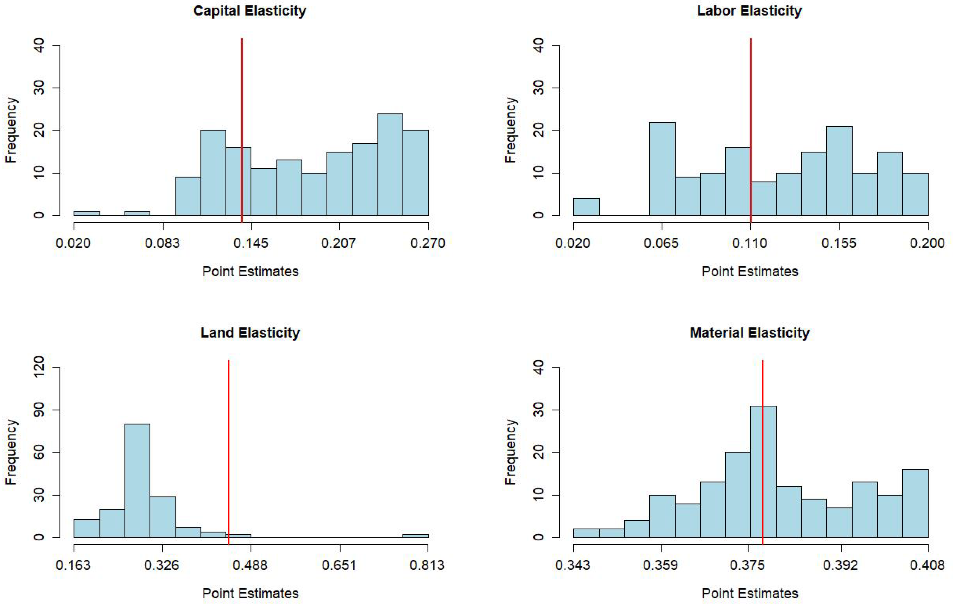
Capital	0.183	0.119	0.201	0.237	0.139
	(0.109, 0.291)	(0.020, 0.246)	(0.125, 0.320)	(0.140, 0.390)	(0.095, 0.185)
Labor	0.079	0.062	0.090	0.130	0.110
	(0.041, 0.140)	(0.020, 0.140)	(0.026, 0.166)	(0.070, 0.231)	(0.051, 0.173)
Land	0.263	0.214	0.243	0.264	0.447
	(0.036, 0.373)	(0.021, 0.396)	(0.009, 0.359)	(0.031, 0.316)	(0.364, 0.521)
Materials	0.38	0.367	0.38	0.398	0.378
	(0.371, 0.395)	(0.35, 0.386)	(0.367, 0.399)	(0.392, 0.416)	(0.360, 0.398)

The left panel summarizes point estimates of ${\beta }_{\kappa }\left(s_i\right)\forall \kappa \in \{K,L,N,M\}$ with the corresponding two-sided 95% bias-corrected confidence intervals in parentheses. The right panel reports their counterparts from a fixed-coefficient location-invariant model.

reports the location-varying input elasticities. The input elasticity of materials is the largest, with a mean (median) value of 0.380 (0.380). The second-largest input elasticity is for land with a mean (median) input elasticity of 0.263 (0.243), while for capital the elasticity is 0.183 (0.201). Labor has an input elasticity at the mean (median) of 0.079 (0.090). We observe significantly different elasticity estimates between quartiles. Within the interquartile interval of their point estimates, the elasticities of capital, labor, land, and materials increase by 0.118, 0.068, 0.050, and 0.031, which correspond to changes of 99%, 110%, 23%, and 8%, respectively.

The right panel of Table 2 reports the results of the fixed-coefficient location-invariant model (that is, not locationally varying), with the corresponding two-sided 95% bias-corrected confidence intervals in parentheses. The fixed-coefficient location-invariant model, which assumes a constant production relationship across all locations, is estimated by allowing the bandwidths in both the first step ($h_1$) and the second step ($h_2$) to diverge towards infinity. This effectively assigns equal weights to all data points, irrespective of their location. When comparing the mean values of the locationally varying model to the fixed-coefficient model, some notable differences emerge. The coefficient for capital is relatively smaller in the fixed-coefficient model, while the coefficients for land are larger. On the other hand, the coefficients for materials and labor remain relatively similar between the two models.

From Figure 2, we can visualize the variation in the input elasticities of grain farmers in different locations in Norway. Location-invariant estimates (from the fixed-coefficient location-invariant model) are depicted by vertical lines. Consistent with the figures in Table 2, all distributions exhibit a wide spread, and the locationally homogeneous model (i.e., the location-invariant fixed coefficient model) appears to be unable to provide a reasonable representation of the production technology across different regions.

Table 3. Locationally varying returns to scale estimates.

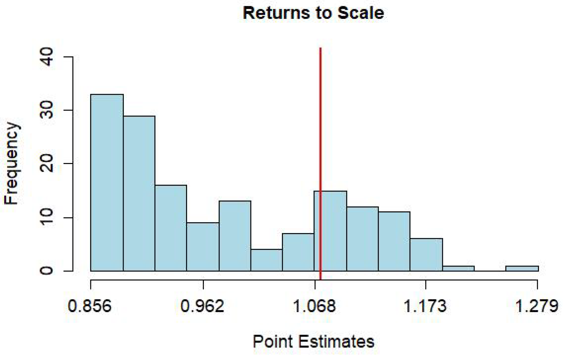
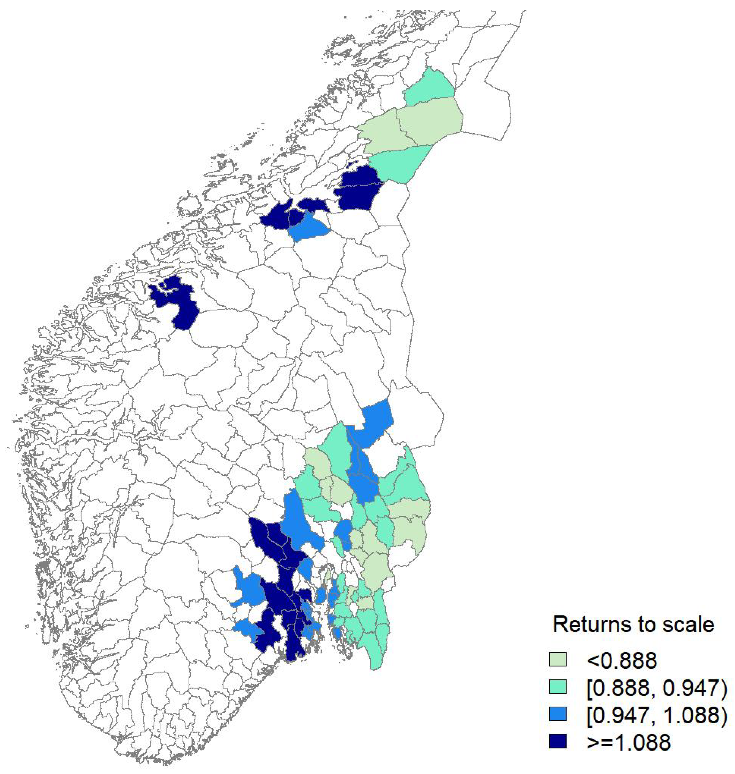
	Mean	1st Qu.	Median	3rd Qu.	<1	=1	>1
RTS	0.926	0.833	0.911	1.011	26.29	74.86	4.57
	(0.762, 1.110)	(0.655, 0.995)	(0.700, 1.079)	(0.830, 1.206)

The left panel summarizes point estimates of ${\sum }_{\kappa }{\beta }_{\kappa }\left(s_i\right)$, with $\kappa \in \{K,L,N,M\}$ with the corresponding two-sided 95% bias-corrected confidence intervals in parentheses. The counterpart estimate of the returns to scale from a fixed-coefficient location-invariant model is 1.074 (1.009, 1.151). The right panel reports the shares of locations in which location-specific point estimates are (i) statistically less than 1 (decreasing returns to scale), (ii) not significantly different from 1 (constant returns to scale), and (iii) statistically greater than 1 (increasing returns to scale). The former classification is based on a two-sided test, the latter on a one-sided test.

presents summary statistics of the estimated returns to scale (RTS) derived from our location-varying production function model. Additionally, Figure 3 provides a corresponding plot that visually displays these estimates. The mean (median) RTS is 0.926 (0.911), with an interquartile range of 0.178, which corresponds to a change of 21%. Figure 3 also illustrates that single-point RTS estimates with the fixed-coefficient location-invariant model (the vertical line) will be less representative estimates of the sample analyzed.

In the right panel of Table 3, the fraction of Norwegian grain farms that exhibit decreasing, constant, or increasing RTS is reported. The classification is based on the RTS point estimates being statistically lower than, equal to, or larger than one, respectively, at the significance level 5%. In most of the locations in Norway with grain farming, we find that the farms exhibit constant RTS. These findings are consistent with other studies by Norwegian grain farmers over the period 1991 to 2005 (e.g., Lien et al. 2010). However, note that, in our study, more than 26% of farms provide evidence of decreasing returns to scale, and almost 5% of farms exhibit increasing returns to scale.

Figure 4 shows the locational heterogeneity in production technology for Norwegian grain farming according to the plot of the RTS estimates (only in locations with grain farming). The map shows quite large differences, but there does not appear to be any systematic pattern in the level of RTS across the country. Considering that adjacent lands typically share similarities in unobserved factors like soil type and climate, we initially anticipated a gradual change in production technology in different locations. However, our findings do not align with this behavior. Despite identifying location-heterogeneous production functions, we did not observe any discernible patterns of productivity differences between locations. Therefore, while we did find support for the existence of diverse production functions in different areas, their distribution did not reveal any consistent trends or spatial correlations throughout the country.

5.2. Productivity Process

The left panel of

Table 4. Productivity process coefficient estimates.

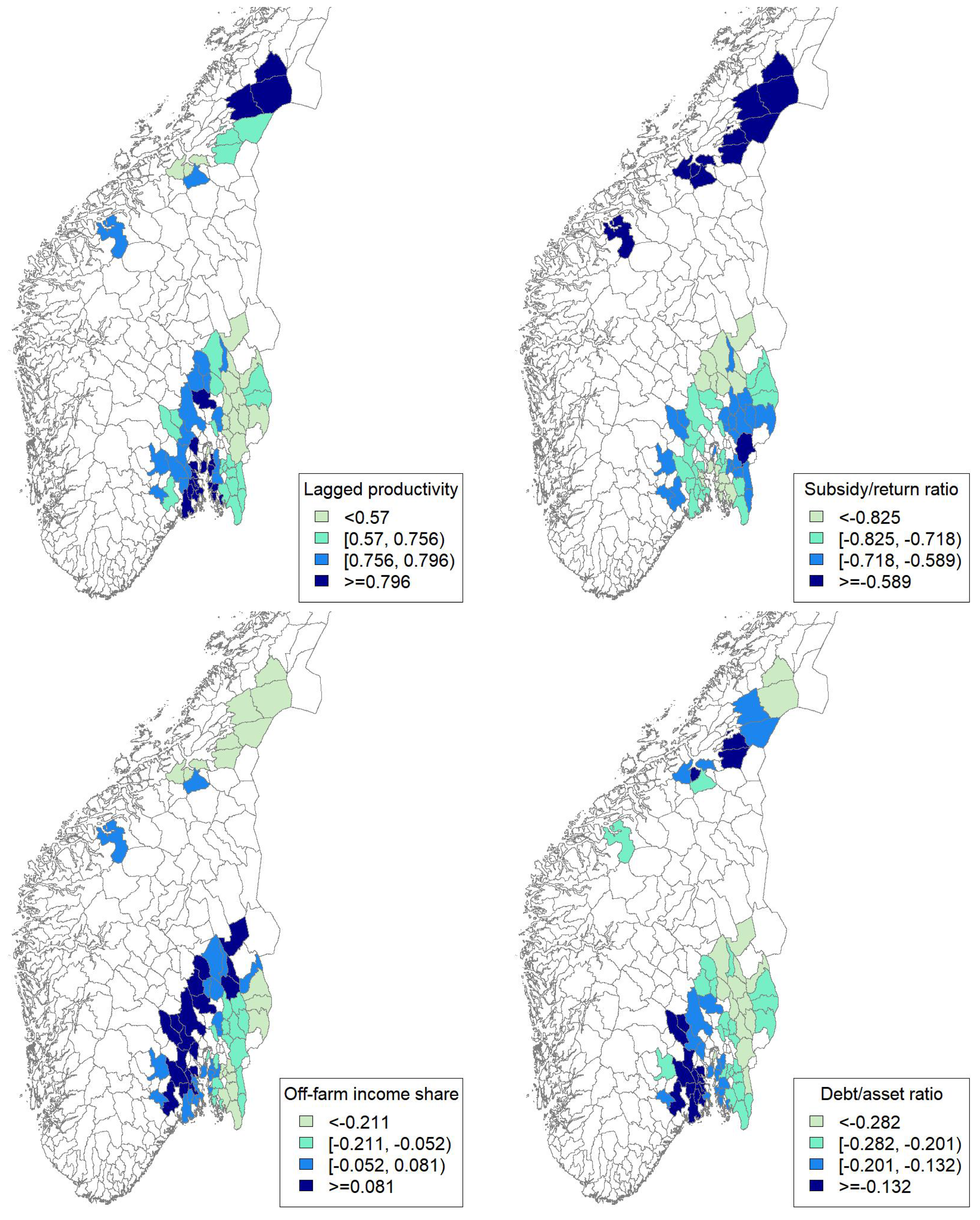
	Locationally Varying						Location-Invariant
Variables	Mean	1st Qu.	Median	3rd Qu.	>0	<0	Point Estimate
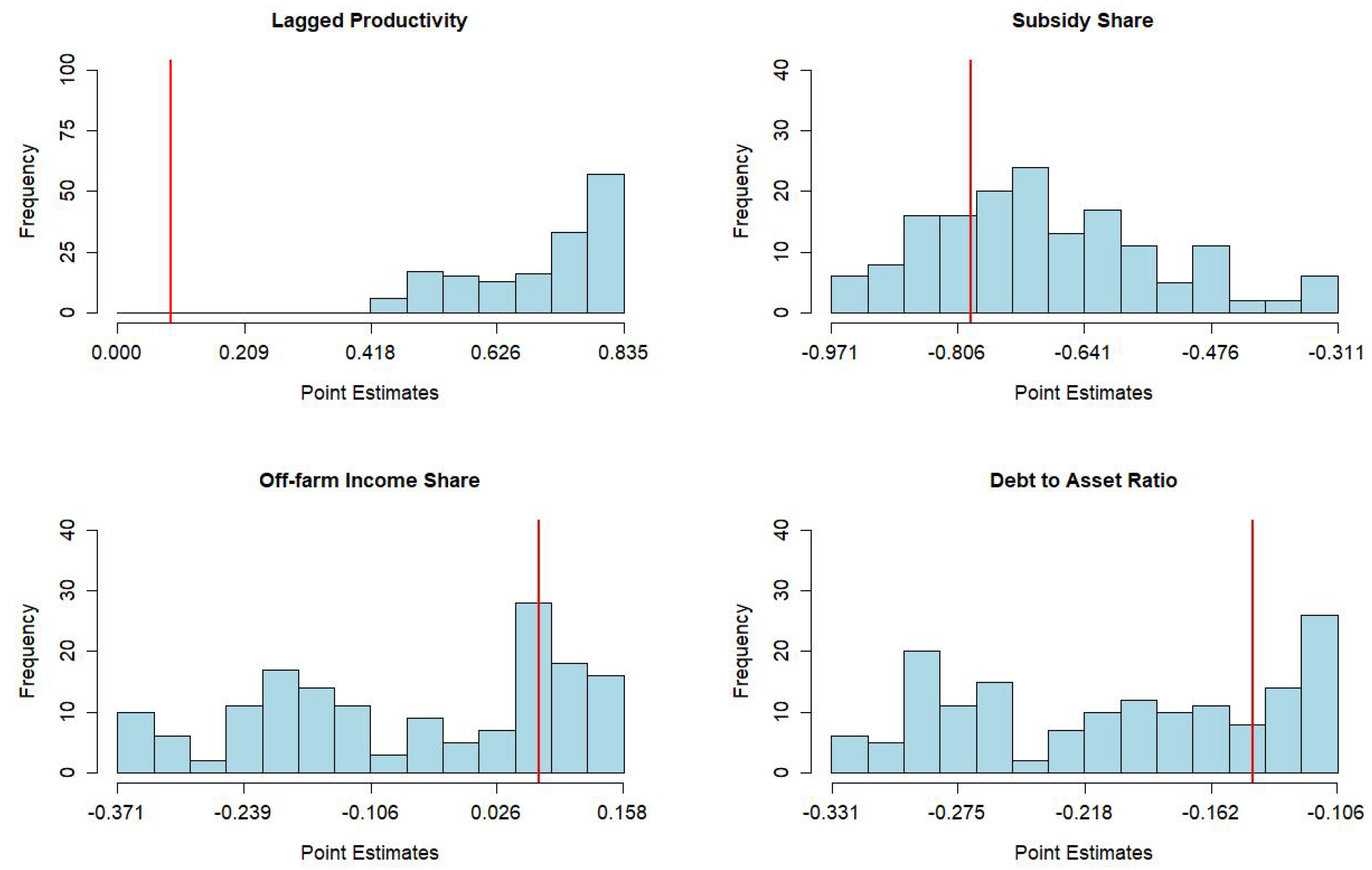
Lagged	0.789	0.734	0.835	0.877	100	0	0.088
productivity	(0.522, 0.976)	(0.609, 0.983)	(0.592, 1.057)	(0.471, 1.078)			(−0.037, 0.200)
Subsidy/return	−0.640	−0.803	−0.688	−0.475	0	73.71	−0.789
ratio	(−0.714, −0.301)	(−0.886, −0.502)	(−0.775, −0.411)	(−0.593, −0.043)			(–1.086, −0.517)
Off-farm	−0.098	−0.217	−0.085	0.057	1.14	32	0.070
income share	(−0.307, 0.012)	(−0.431, −0.022)	(−0.296, 0.000)	(−0.198, 0.150)			(−0.089, 0.303)
Debt/asset	−0.222	−0.292	−0.216	−0.104	0	63.43	−0.143
ratio	(−0.334, −0.072)	(−0.403, −0.109)	(−0.342, −0.079)	(−0.264, 0.019)			(−0.264, −0.013)

The left panel summarizes point estimates of ${\lambda }_j\left(s_i\right)\forall j=1,\dots ,dim\left(X\right)$, with the corresponding two-sided 95% bias-corrected confidence intervals in parentheses. The reports also report a share of locations in which location-specific point estimates are statistically positive or negative via a one-sided test. The right panel reports the counterparts of a fixed-coefficient location-invariant model.

presents the estimate of the marginal effects, varying locationally, of the productivity determinants in the evolution process of ${\omega }_{it}$. The corresponding two-sided 95% bias-corrected confidence intervals are shown in parentheses. Additionally, the final columns of the left panel indicate the share of locations where location-specific point estimates are statistically positive or negative at the 5% significance level, determined through a one-sided test. The right panel of Table 4 displays the marginal effects of the productivity determinants in the fixed-coefficient location-invariant model.

The spatial autoregressive coefficient of lagged productivity, as the measure of persistent productivity, is at the mean (median) 0.789 (0.835). This means that a farm’s future productivity will on average increase by 0.789% if the farm’s past productivity increases by 1%, ceteris paribus. However, we observe differences in productivity between locations/regions. Within the interquartile interval of their point estimates, lagged productivity increases by 0.145, which in turn corresponds to a 20% change. The upper left panel of Figure 5 also illustrates the variation between locations in the estimated lagged productivity, which roughly varies between 0.50 and 0.90, while most locations/regions have a large spatial autoregressive coefficient of around 0.80. The lagged productivity estimate of the location-invariant model with fixed coefficient is depicted by a vertical line (in Figure 5) and is far from the estimates of the location-varying model.

As reported in Table 4, for farms in most locations (73.71%), the subsidy/income ratio has a significantly negative effect on productivity, while for 26.29% (100–73.71%) of the locations, the subsidy/income ratio has no effect on farm productivity. For the whole sample, a 1% point increase in the subsidy/income ratio is associated with a reduction in the next period’s farm productivity by about 0.65% points on average. In this sense, our result supports Kumbhakar and Lien (2010). In a study of Norwegian grain farms during 1991–2006, they found that an increase in subsidy payment reduced production. Zhengfei and Lansink (2006) also found that subsidies had a negative impact on productivity growth in Dutch arable farming during the period 1990–1999. However, our result partly contrasts with the findings of Rizov et al. (2013). In their study on mixed farms in 15 EU countries from 1990 to 2008, Rizov et al. (2013) observed that subsidies had a negative impact on productivity prior to the implementation of the decoupling reform in 2003. However, after the decoupling reform, the effect of subsidies on productivity became positive in several countries. As discussed in Rizov et al. (2013), subsidies can both increase and reduce productivity, and the net effect is not obvious. As the upper right panel of Figure 5 illustrates, our locationally varying estimation model also exhibits quite a large locational variation in the effect of the subsidy/income ratio on productivity.

Point estimates of off-farm income share effects on productivity are negative in 32% of the locations, but statistically insignificant in approximately 67% of the locations (Table 4). These results are not unexpected. The impact of off-farm work on farm productivity is multifaceted. On the one hand, participating in non-farm work can provide farmers with valuable experiences and skills that enhance farm management practices and overall productivity. In addition, extra income from off-farm work may facilitate investments in technologies that increase farm output. On the other hand, reduced on-farm participation due to off-farm work may lead to less efficient use of resources, potentially resulting in lower output.

The influence of off-farm work on productivity can also vary between regions due to differences in agricultural and climatic conditions, as well as variations in off-farm job markets. Our empirical findings support this notion, as depicted in the lower left panel of Figure 5. In a study that focused on Norwegian grain farms from 1991 to 2005, Lien et al. (2010) discovered that the effect of off-farm work on productivity exhibits an inverted U shape. Initially, some off-farm work had a positive impact on productivity, while excessive off-farm work had a negative effect. In general, the relationship between off-farm work and farm productivity is complex, and its implications can vary depending on factors such as the nature of off-farm employment, regional characteristics, and the level of farmer participation in both on-farm and off-farm activities. Given off-farm work is almost the norm among today’s Norwegian grain farmers (cf., Table 1), our results are more or less consistent with the findings of Lien et al. (2010). We also mention, as examples, that Goodwin and Mishra (2004) with U.S. family farms and Pfeiffer et al. (2009) with Mexican farms found that greater participation in off-farm labor markets decreased on-farm efficiency and productivity.

The effects of the debt/asset ratio are also negative on productivity for about two-thirds of the locations/regions, but statistically insignificant for about one-third. On average, a 1% point increase in the debt/asset ratio is associated with a reduction in the next period’s productivity by about 0.22% points. In terms of a related study of Norwegian grain farms, Kumbhakar and Lien (2010) concluded that a higher debt/asset ratio suggested a decrease in technical efficiency. As a decrease in technical efficiency implies reduced productivity, their results are consistent with ours.

Figure 6 and Figure 7 illustrate the geographical variation in productivity estimates. However, unlike the expected gradual change or systematic pattern across different locations as shown in Figure 4 for the RTS estimates, the productivity estimate maps do not show any clear trends. This discrepancy suggests that our current approach of employing unobserved locationally heterogeneous production functions might not be the most appropriate method to address possible patterns in productivity, if any, across different locations. Further exploration and alternative methodologies may be necessary to better capture and understand the underlying factors contributing to the observed variations in productivity at different locations.

However, it is important to emphasize that this finding does not diminish the significance of our approach, as our primary objective is to investigate and understand heterogeneity. While our method might not directly reveal patterns in productivity across locations, it does shed valuable light on the presence of heterogeneity in the data. This insight is crucial in itself, as it highlights the diverse nature of productivity in different areas, which can be a critical aspect in various fields, such as regional economic development, policy formulation, and resource allocation. In this context, our approach remains valuable for providing a deeper understanding of the complexities and variations within the studied system, even if it does not directly address specific spatial patterns in productivity.

6. Concluding Remarks

By comparing farms, it is easy to observe that agriculture is a heterogeneous industry in terms of the natural land characteristics that determine natural advantage (such as soil type, fertility, the slope of the land, the climate, etc.) and that, as a consequence, there can be huge differences from region to region within a country (or other geographical unit). Furthermore, the interaction between site-specific environmental variables and farmer decision-making regarding technology can promote the development of locally specific varieties and technologies. As a result, a diverse technological landscape may emerge characterized by the existence of various spatial regimes in technologies. Together, these call for spatial analysis or, more specifically, for analyses that account for spatial dependency and/or spatial heterogeneity. In the agricultural economics literature, these are often ignored,7 as a global model is often fitted to all the farms included in a given sample. When important and relevant relationships vary over space, global parameter estimates may be misleading and can lead to less reliable economic conclusions.

This paper seeks to bridge the existing gap in the literature by investigating firm/farm- and location-specific heterogeneity. We introduce a semiparametric methodology that facilitates the identification of production functions, considering the diverse effects of the firm’s/farm’s production technology and productivity evolution. Inspired by the recent work of Malikov et al. (2022), our novel model explicitly incorporates spatial variation in the estimation of production function parameters, encompassing input elasticities and productivity parameters.

We investigate the efficacy of using longitude/latitude locations to capture variations between firms and locations within the Norwegian grain farming sector. Our methodology offers a practical tool for investigating how variations across locations contribute to regional or local productivity disparities and the underlying factors driving these differences. We find evidence of locationally heterogeneous production functions but no apparent pattern of productivity estimates across different locations. The lack of observable patterns in productivity estimates suggests that there could be other factors or variables that influence productivity variations, which our current approach may not fully capture. Therefore, it would be prudent to explore alternative methodologies that could better account for these underlying factors and provide more comprehensive insights into the spatial distribution of productivity in the studied locations.

In future research, there is ample potential to enhance our firm- and location-specific semiparametric production function approach. An important extension would involve incorporating observed spatial determinants in addition to the GPS coordinates currently used. By addressing our observation in this study that relying solely on longitude/latitude locations to account for spatial industry variations may not always be suitable, this expanded approach could offer a valuable solution. By integrating additional spatial information, such as soil types, climate data, or terrain characteristics, we can refine the analysis and capture a more comprehensive picture of the spatial heterogeneity present in the industry. This enhanced methodology would likely yield more accurate and nuanced insights into the complexities of location-specific productivity in various industries.

References

- Ackerberg, Daniel A., Kevin Caves, and Garth Frazer. 2015. Identification properties of recent production function estimators. Econometrica 83: 2411–51. [Google Scholar] [CrossRef]
- Aida, Takeshi. 2018. Neighbourhood effects in pesticide use: Evidence from the rural philippines. Journal of Agricultural Economics 69: 163–81. [Google Scholar] [CrossRef]
- Álvarez, Antonio, Julio Del Corral, Daniel Solís, and José A. Pérez. 2008. Does intensification improve the economic efficiency of dairy farms? Journal of Dairy Science 91: 3693–98. [Google Scholar] [CrossRef]
- Anselin, Luc. 2010. Thirty years of spatial econometrics. Papers in Regional Science 89: 3–25. [Google Scholar] [CrossRef]
- Bai, Xiuguang, Tianwen Zhang, Shujuan Tian, and Yanan Wang. 2021. Spatial analysis of factors affecting fertilizer use efficiency in China: An empirical study based on geographical weighted regression model. Environmental Science and Pollution Research 28: 16663–681. [Google Scholar] [CrossRef]
- Billé, Anna Gloria, Cristina Salvioni, and Roberto Benedetti. 2018. Modelling spatial regimes in farms technologies. Journal of Productivity Analysis 49: 173–85. [Google Scholar] [CrossRef]
- Blundell, Richard, and Stephen Bond. 2000. GMM estimation with persistent panel data: An application to production functions. Econometric Reviews 19: 321–40. [Google Scholar] [CrossRef]
- Brunsdon, Chris, A. Stewart Fotheringham, and Martin E. Charlton. 1996. Geographically weighted regression: A method for exploring spatial nonstationarity. Geographical Analysis 28: 281–98. [Google Scholar] [CrossRef]
- Canello, Jacopo, and Francesco Vidoli. 2020. Investigating space-time patterns of regional industrial resilience through a micro-level approach: An application to the italian wine industry. Journal of Regional Science 60: 653–76. [Google Scholar] [CrossRef]
- Capello, Roberta. 2009. Space, growth and development. In Handbook of Regional Growth and Development Theories. Cheltenham: Edward Elgar Publishing. [Google Scholar]
- Chen, Xiaohong. 2007. Large sample sieve estimation of semi-nonparametric models. In Handbook of Econometrics. Amsterdam: Elsevier, vol. 6, pp. 5549–632. [Google Scholar]
- Collard-Wexler, Allan, and Jan De Loecker. 2015. Reallocation and technology: Evidence from the US steel industry. American Economic Review 105: 131–71. [Google Scholar] [CrossRef]
- De Loecker, Jan. 2013. Detecting learning by exporting. American Economic Journal: Microeconomics 5: 1–21. [Google Scholar] [CrossRef]
- Doraszelski, Ulrich, and Jordi Jaumandreu. 2013. R&D and productivity: Estimating endogenous productivity. Review of Economic Studies 80: 1338–83. [Google Scholar]
- Doraszelski, Ulrich, and Jordi Jaumandreu. 2018. Measuring the bias of technological chance. Journal of Political Economy 126: 1027–84. [Google Scholar] [CrossRef]
- Dosi, Giovanni, and Richard R. Nelson. 2010. Technical change and industrial dynamics as evolutionary processes. In Handbook of the Economics of Innovation. Amsterdam: Elsevier, vol. 1, pp. 51–127. [Google Scholar]
- Eberhardt, Markus, and Francis Teal. 2013. No mangoes in the Tundra: Spatial heterogeneity in agricultural productivity analysis. Oxford Bulletin of Economics and Statistics 75: 914–39. [Google Scholar] [CrossRef]
- Efron, Bradley. 1987. Better bootstrap confidence intervals. Journal of the American Statistical Association 82: 171–85. [Google Scholar] [CrossRef]
- Fusco, Elisa, and Francesco Vidoli. 2013. Spatial stochastic frontier models: Controlling spatial global and local heterogeneity. International Review of Applied Economics 27: 679–94. [Google Scholar] [CrossRef]
- Gandhi, Amit, Salvador Navarro, and David A. Rivers. 2020. On the identification of gross output production functions. Journal of Political Economy 128: 2973–3016. [Google Scholar] [CrossRef]
- Goodwin, Barry K., and Ashok K. Mishra. 2004. Farming efficiency and the determinants of multiple job holding by farm operators. American Journal of Agricultural Economics 86: 722–29. [Google Scholar] [CrossRef]
- Greene, William. 2005. Reconsidering heterogeneity in panel data estimators of the stochastic frontier model. Journal of Econometrics 126: 269–303. [Google Scholar] [CrossRef]
- Holmes, Thomas J., and Sanghoon Lee. 2012. Economies of density versus natural advantage: Crop choice on the back forty. Review of Economics and Statistics 94: 1–19. [Google Scholar] [CrossRef]
- Isard, Walter. 1954. Location theory and trade theory: Short-run analysis. The Quarterly Journal of Economics 68: 305–20. [Google Scholar] [CrossRef]
- Just, Richard E., and Rulon D. Pope. 2001. The agricultural producer: Theory and statistical measurement. In Handbook of Agricultural Economics. Amsterdam: Elsevier, vol. 1, pp. 629–741. [Google Scholar]
- Knutsen, Heidi. 2020 Norwegian Agriculture Status and Trends 2019. NIBIO POP. 6. Available online: http://hdl.handle.net/11250/2643268 (accessed on 13 February 2023).
- Konings, Jozef, and Stijn Vanormelingen. 2015. The impact of training on productivity and wages: Firm-level evidence. Review of Economics and Statistics 97: 485–97. [Google Scholar] [CrossRef]
- Kumbhakar, Subal C., and Efthymios G. Tsionas. 2010. Estimation of production risk and risk preference function: A nonparametric approach. Annals of Operations Research 176: 369–78. [Google Scholar] [CrossRef]
- Kumbhakar, Subal C., and Gudbrand Lien. 2010. Impact of subsidies on farm productivity and efficiency. In The Economic Impact of Public Support to Agriculture. Edited by V. Eldon Ball, Roberto Fanfani and Luciano Gutierrez. Berlin/Heidelberg: Springer, pp. 109–24. [Google Scholar]
- Läpple, Doris, and Hugh Kelley. 2015. Spatial dependence in the adoption of organic drystock farming in ireland. European Review of Agricultural Economics 42: 315–37. [Google Scholar] [CrossRef]
- Läpple, Doris, Garth Holloway, Donald J. Lacombe, and Cathal O’Donoghue. 2017. Sustainable technology adoption: A spatial analysis of the irish dairy sector. European Review of Agricultural Economics 44: 810–35. [Google Scholar]
- Levinsohn, James, and Amil Petrin. 2003. Estimating production functions using inputs to control for unobservables. Review of Economic Studies 70: 317–41. [Google Scholar] [CrossRef]
- Li, Qi, Cliff J. Huang, Dong Li, and Tsu-Tan Fu. 2002. Semiparametric smooth coefficient models. Journal of Business & Economic Statistics 20: 412–22. [Google Scholar]
- Lien, Gudbrand, Subal C. Kumbhakar, and J. Brian Hardaker. 2010. Determinants of off-farm work and its effects on farm performance: The case of norwegian grain farmers. Agricultural Economics 41: 577–86. [Google Scholar] [CrossRef]
- Malikov, Emir, and Gudbrand Lien. 2021. Proxy variable estimation of multiproduct production functions. American Journal of Agricultural Economics 103: 1878–902. [Google Scholar] [CrossRef]
- Malikov, Emir, and Shunan Zhao. 2021. On the estimation of cross-firm productivity spillovers with an application to fdi. Review of Economics and Statistics. forthcoming. [Google Scholar] [CrossRef]
- Malikov, Emir, Jingfang Zhang, Shunan Zhao, and Subal C. Kumbhakar. 2022. Accounting for cross-location technological heterogeneity in the measurement of operations efficiency and productivity. Journal of Operations Management 68: 153–84. [Google Scholar] [CrossRef]
- Malikov, Emir, Shunan Zhao, and Subal C. Kumbhakar. 2020. Estimation of firm-level productivity in the presence of exports: Evidence from China’s manufacturing. Journal of Applied Econometrics 35: 457–80. [Google Scholar] [CrossRef]
- McMillen, Daniel P., and Christian L. Redfearn. 2010. Estimation and hypothesis testing for nonparametric hedonic house price functions. Journal of Regional Science 50: 712–33. [Google Scholar] [CrossRef]
- Mundlak, Yair. 2001. Production and supply. In Handbook of Agricultural Economics. Amsterdam: Elsevier, vol. 1, pp. 3–85. [Google Scholar]
- O’Donnell, Christopher John, and William E. Griffiths. 2006. Estimating state-contingent production frontiers. American Journal of Agricultural Economics 88: 249–66. [Google Scholar] [CrossRef]
- Olley, G. Steven, and Ariel Pakes. 1996. The dynamics of productivity in the telecommunications equipment industry. Econometrica 64: 1263–97. [Google Scholar] [CrossRef]
- Orea, Luis, and Subal C. Kumbhakar. 2004. Efficiency measurement using a latent class stochastic frontier model. Empirical Economics 29: 169–83. [Google Scholar] [CrossRef]
- Pfeiffer, Lisa, Alejandro López-Feldman, and J. Edward Taylor. 2009. Is off-farm income reforming the farm? Evidence from Mexico. Agricultural Economics 40: 125–38. [Google Scholar] [CrossRef]
- Postiglione, Paolo, Roberto Benedetti, and Federica Piersimoni. 2022. Spatial Econometric Methods in Agricultural Economics Using R. Boca Raton: CRC Press. [Google Scholar]
- Rizov, Marian, Jan Pokrivcak, and Pavel Ciaian. 2013. CAP subsidies and productivity of the EU farms. Journal of Agricultural Economics 64: 537–57. [Google Scholar] [CrossRef]
- Saint-Cyr, Legrand D. F., Hugo Storm, Thomas Heckelei, and Laurent Piet. 2019. Heterogeneous impacts of neighbouring farm size on the decision to exit: Evidence from brittany. European Review of Agricultural Economics 46: 237–66. [Google Scholar] [CrossRef]
- Sauer, Johannes, and Catherine J. Morrison Paul. 2013. The empirical identification of heterogeneous technologies and technical change. Applied Economics 45: 1461–79. [Google Scholar] [CrossRef]
- Schmidtner, Eva, Christian Lippert, Barbara Engler, Anna Maria Häring, Jaochim Aurbacher, and Stephan Dabbert. 2012. Spatial distribution of organic farming in germany: Does neighbourhood matter? European Review of Agricultural Economics 39: 661–83. [Google Scholar] [CrossRef]
- Skevas, Theodoros, Ioannis Skevas, and Scott M. Swinton. 2018. Does spatial dependence affect the intention to make land available for bioenergy crops? Journal of Agricultural Economics 69: 393–412. [Google Scholar] [CrossRef]
- Storm, Hugo, Klaus Mittenzwei, and Thomas Heckelei. 2015. Direct payments, spatial competition, and farm survival in norway. American Journal of Agricultural Economics 97: 1192–205. [Google Scholar] [CrossRef]
- Syverson, Chad. 2011. What determines productivity? Journal of Economic Literature 49: 326–65. [Google Scholar] [CrossRef]
- Ullah, Amman. 1985. Specification analysis of econometric models. Journal of Quantitative Economics 1: 187–209. [Google Scholar]
- Van Biesebroeck, Johannes. 2005. Exporting raises productivity in sub-Saharan African manufacturing firms. Journal of International Economics 67: 373–91. [Google Scholar] [CrossRef]
- Vidoli, Francesco, Concetta Cardillo, Elisa Fusco, and Jacopo Canello. 2016. Spatial nonstationarity in the stochastic frontier model: An application to the Italian wine industry. Regional Science and Urban Economics 61: 153–64. [Google Scholar] [CrossRef]
- Wang, Haoying. 2018. The spatial structure of farmland values: A semiparametric approach. Agricultural and Resource Economics Review 47: 568–91. [Google Scholar] [CrossRef]
- Zhengfei, Guan, and Alfons Oude Lansink. 2006. The source of productivity growth in dutch agriculture: A perspective from finance. American Journal of Agricultural Economics 88: 644–56. [Google Scholar] [CrossRef]