1. Introduction
Wireless communication technologies can play a significant role in the industrial environment for factory automation to increase productivity and efficiency of the manufacturing systems [
1,
2]. By adding sensors to industrial equipment, wireless sensor networks are often used for data acquisition in Industrial Internet of Things (IIoT). The main advantage of using wireless connections in factory automation is that devices and machines can be moved and connected more freely and no restricting cables are present.
Real-time wireless sensors is one of the building blocks of the recent large-scale I-MECH project [
3,
4], which is fully industry driven initiative trying to enable fast integration of diverse set of components (either electronic systems, software modules, sensors or actuators) for demanding mechatronic applications respecting model-based system engineering principles. In this regard, the modeling library for wireless data acquisition was developed within the aforementioned building block, which deals with robust wireless network providing reliable, synchronized and secure data delivery from sensors to the master node (or central computing unit) in an energy efficient manner. Among a number of different wireless communication technologies (Wi-Fi, ZigBee, Bluetooth, RFID, etc. [
5,
6]), Bluetooth Low Energy (BLE), which is optimized for low power communication [
7], was selected as the most appropriate solution satisfying the majority of identified requirements. These include low latency (less than 500 us) and fast update rates (at least 1.6 kHz), which are necessary for advanced control strategies exploiting auxiliary load-side measurements.
With the release of Bluetooth v4.0, the BLE protocol was introduced in 2010. It was designed to be ultra-low power and low cost technology for short-range communications, and was targeted at monitoring and control applications that require devices to send small amounts of data from once a second to once every few days [
7]. Few examples are energy management for smart homes [
8], sensor-based healthcare systems [
9] and indoor positioning systems [
10].
Over time, different aspects of the protocol have been analyzed (e.g., throughput [
11,
12], energy consumption [
13], delay performance for connection-oriented applications [
14], neighbor discovery process [
15], channel utilization and the adaptive frequency hopping scheme [
16]), including BLE suitability for IIoT applications [
17,
18,
19] and proposed solutions to meet the real-time demands set for IIoT [
19,
20]. For example, in [
17], the reliability of BLE for industrial wireless sensor and actuator networks is evaluated by studying a point-to-point link based on the physical layers 1M and 2M of BLE under different wireless channels, while in [
18] the potential of BLE for industrial automation is explored by testing the hardware in metal enclosure with different antennas and varying transmitting power. In [
19], the suitability of BLE for time-critical IIoT applications is evaluated showing that by optimally modifying the BLE retransmission scheme, it is possible to ensure reliability and timeliness requirements of IIoT applications, while in [
20] the real-time communication problem is solved for Bluetooth mesh networks by proposing a multi-hop real-time BLE protocol, which is developed on top of BLE to obtain bounded packet delays over mesh networks.
Although many studies have been published on the BLE protocol, only one simulation tool [
21,
22] for investigating the network-level performance has been reported till 2019, when the “Communications Toolbox™ Library for the Bluetooth Protocol” was first introduced with R2019a release of MATLAB [
23]. While the former tool allows to simulate the lower layers (primarily, the Physical and Link Layers) of the BLE protocol and supports only one active link at a time for each simulated device, the latter provides more functionality covering all the layers of BLE stack.
In this paper, the BLE wireless sensor network library, developed in MATLAB (R2017b) Simulink for its support of model-based design, is described (the development of the library started in 2017 when the aforementioned Toolbox library was not yet available; therefore, the proposed library, which was almost completed by the mid of 2019, uses none of the elements from the released library). Different parameters defined by the BLE protocol are explained for the configurable BLE devices (either masters or slaves) with the masters supporting either one or multiple active links at a time depending on the required sampling rate of the sensors connected to the slaves. By considering that high sampling rates (at least 1.6 kHz) and low latencies (less than 500 us) can be achieved only in the connection-oriented mode, the devices in the networks can be connected only in star topologies. Shared slaves and master/slave devices are not supported. The developed tool allows to simulate the Physical and Link Layers of the networks using a fixed-step (1 us) discrete solver. The Physical Layer is responsible for transmission and reception of raw bit streams over a physical medium, while the Link Layer defines how two devices can use a radio to transmit information between one another [
7]. These two layers form the controller part of the BLE protocol stack, which also contains the host residing above the controller. The host is responsible for higher level functionalities, and is not implemented by the library; therefore, is left out of the discussion.
The advantage of the developed library is that it is compatible with earlier versions of MATLAB (2017a), it provides complete blocks of the master and slave devices, which can be conveniently placed and configured in the models, and the provided function new_BLE_model (explained later) allows fast creation of the networks by taking into account the distances between the devices to calculate the attenuation coefficients of the transmitted signals.
The rest of the paper is organized as follows.
Section 2 describes the configurable elements of the library including a function for creating the initial BLE models.
Section 3 provides two examples of the networks demonstrating the operation of the master device in one slave and multiple slaves modes, while the conclusions are given in
Section 4.
2. Library Description
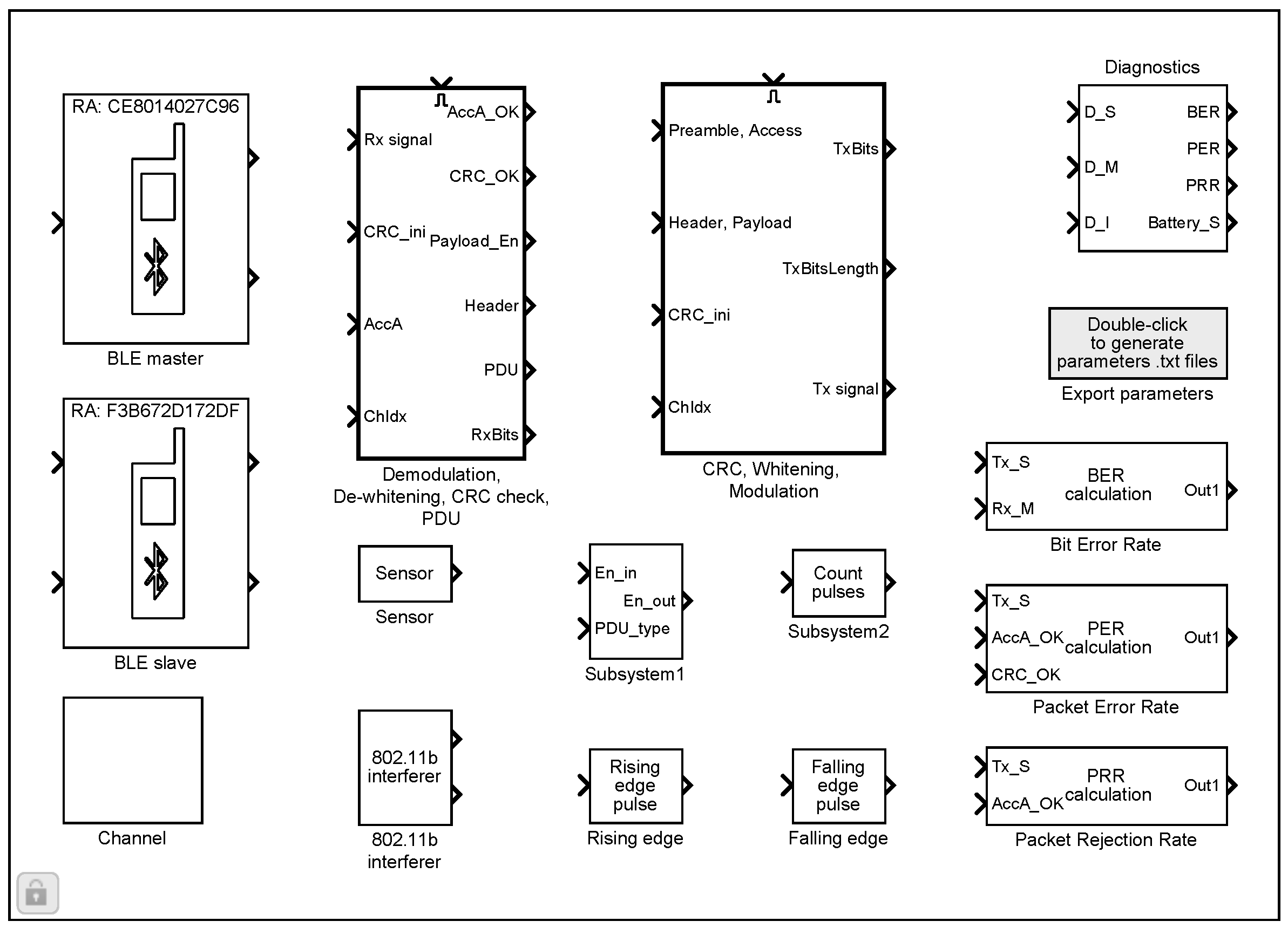
The BLE wireless sensor network library (
Figure 1) allows to build the models for simulating the communication between multiple BLE devices. The library includes configurable blocks of BLE master and slave devices, a sensor, an 802.11b interferer, a transmission channel and a diagnostics block. For creating the initial BLE models, a special MATLAB function (explained in
Section 2.8) can be used, which allows specifying the locations of the devices to determine the distances between them and the corresponding path attenuations of the transmitted signals.
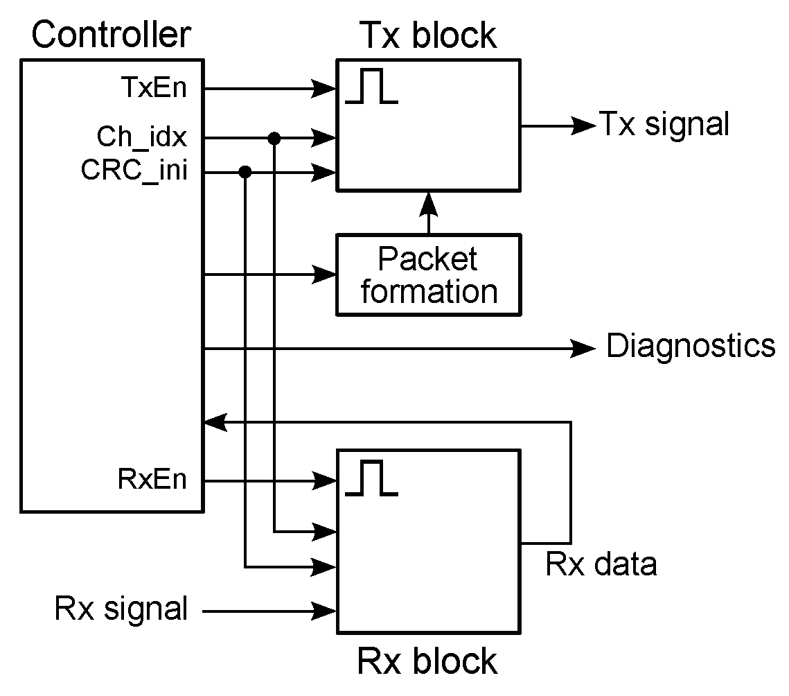
The key elements of the library are the BLE master and slave devices, the common internal block diagram of which is shown in
Figure 2. The operation of the devices is controlled by a Stateflow chart (controller), which enables or disables the transmitter (Tx) and receiver (Rx) blocks (only one block can be active at a time), sets the channel index in the range from 0 to 39 (indices 37, 38 and 39 are used for 3 primary advertising channels with center frequencies 2402, 2426 and 2480 MHz, respectively, while the indices from 0 to 10 and from 11 to 36 are used for 37 data channels with center frequencies
,
and
,
, respectively [
24] p. 2864), initializes a linear feedback shift register for CRC (cyclic redundancy check) generation, controls the formation of the packets, etc. The Tx block is responsible for bit stream processing (CRC generation, whitening [
24] p. 2923) and formation of the radio frequency (RF) signal—the BLE system operates in the 2.4 GHz ISM band and uses 40 RF channels with center frequencies
MHz, where
; the modulation is Gaussian Frequency Shift Keying (GFSK) with a bandwidth-bit period product BT
and a modulation index 0.5 ([
24] p. 2833); a binary one and zero are represented by +250 kHz and −250 kHz frequency deviations, respectively, while a symbol rate is 1 Msym/s. The Rx block demodulates the received signal and performs dewhitening and CRC checking operations. At packet reception, the Access Address is checked first. If the Access Address is correct, the packet is considered received, otherwise the packet is rejected. If the CRC is correct, the packet is considered valid, otherwise the packet is rejected ([
24] p. 2923).
For detection of link loss, both the master and the slave use a connection supervision timer, which starts upon entering the Connection State and resets upon reception of a valid data channel packet. If the timer reaches a certain threshold (called a connection supervision timeout), the connection is considered lost. One threshold value equaling 6 times the connection interval is used after entering the Connection State (at this point, the connection is considered to be created), while the other threshold value is used after receiving a data channel packet from the peer device, which leads to the connection that is considered to be established ([
24] p. 2979).
2.1. Master
The master (initiator) block has one input, which is the received signal from the channel, and two outputs. The first output is the transmitted signal, which goes to the channel, while the second output is the diagnostics bus containing different internal signals of the device, which can be displayed on the scope and analyzed.
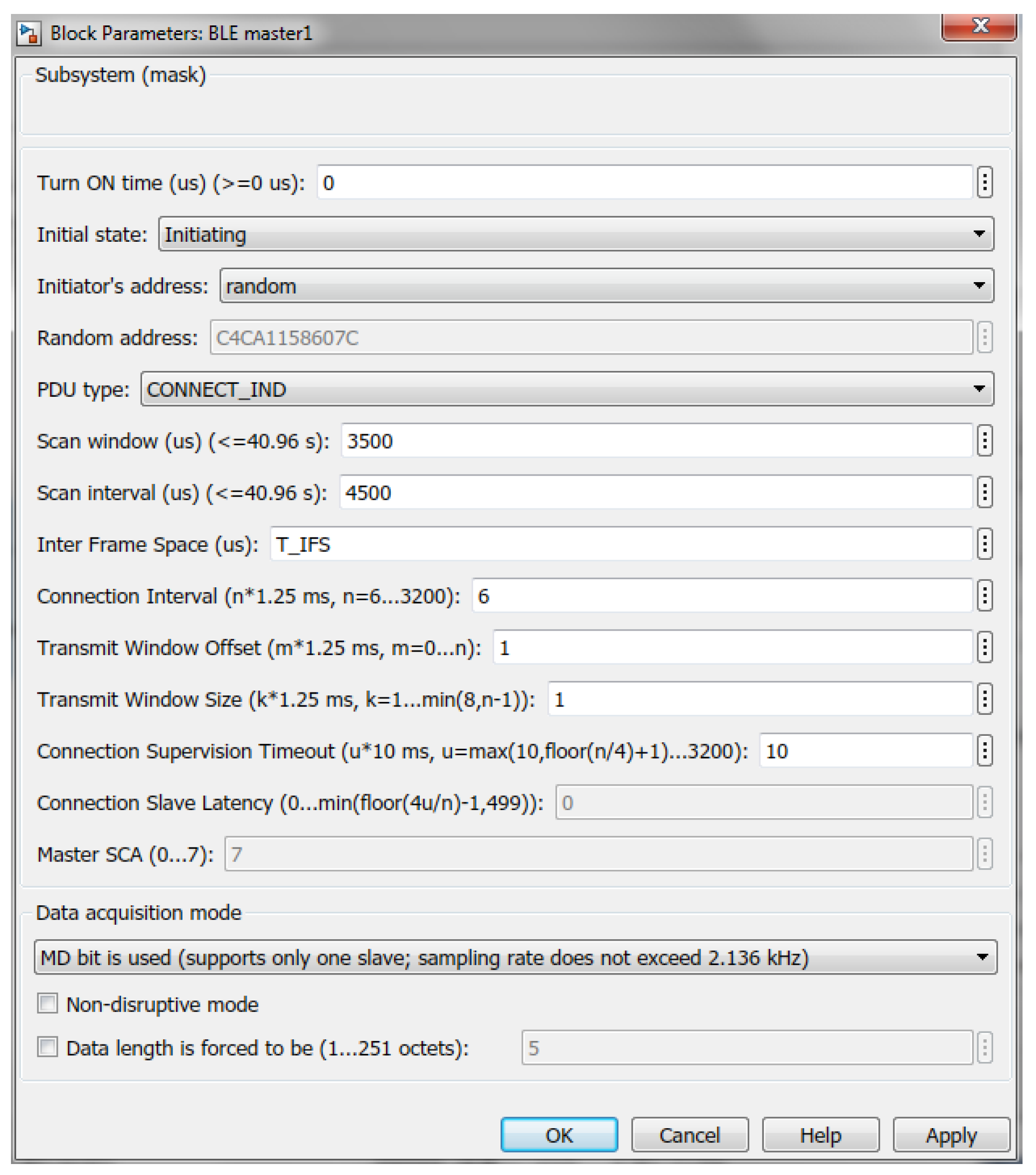
For the master device, the following parameters are configurable (
Figure 3):
Turn ON time—indicates, when the device transitions from the Standby State to the Initiating State (all the implemented sates are shown in Figure 8 on the left);
Initial state—Initiating State (entered at Turn ON time);
Initiator’s address—public (manually entered) or random (generated at placing the block in the model) ([
24] p. 2859);
PDU type—initiating PDU: CONNECT_IND ([
24] p. 2881);
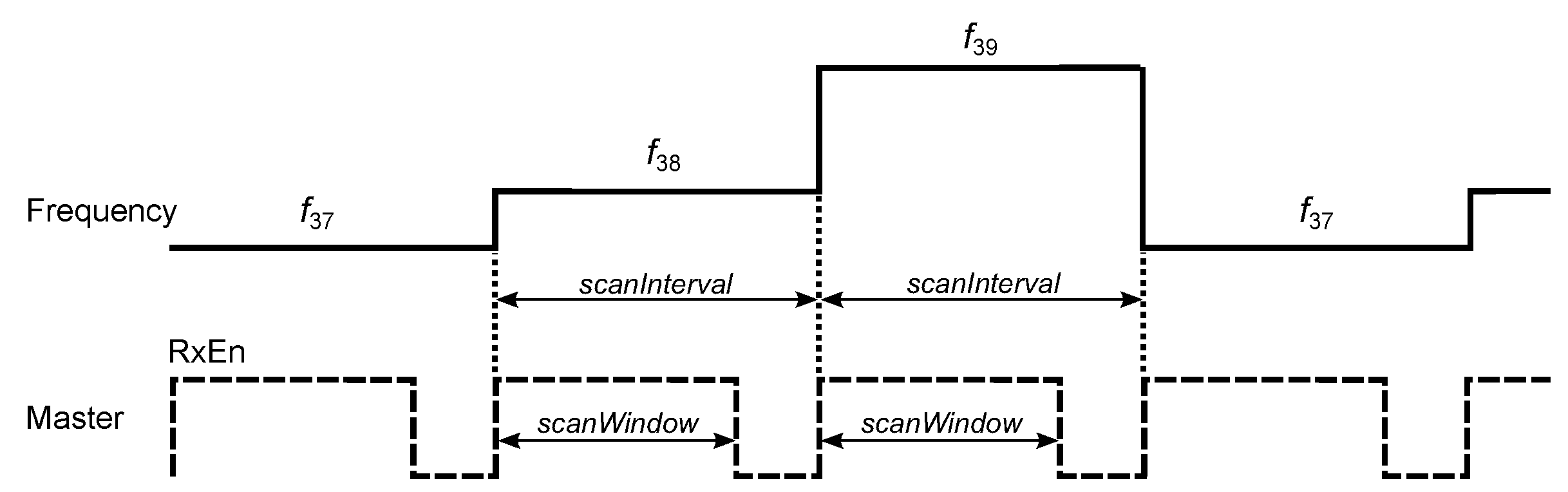
Scan window—after entering the Initiating State, master sequentially listens on the 3 primary advertising channels for the duration of scan window (≤40.96 s) for a connectable advertisement ([
24] p. 2964);
Scan interval—the time interval (≤40.96 s) between the start of two consecutive scan windows (
Figure 4) ([
24] p. 2964);
Inter frame space—the time interval
us between two consecutive packets on the same channel index ([
24] p. 2927);
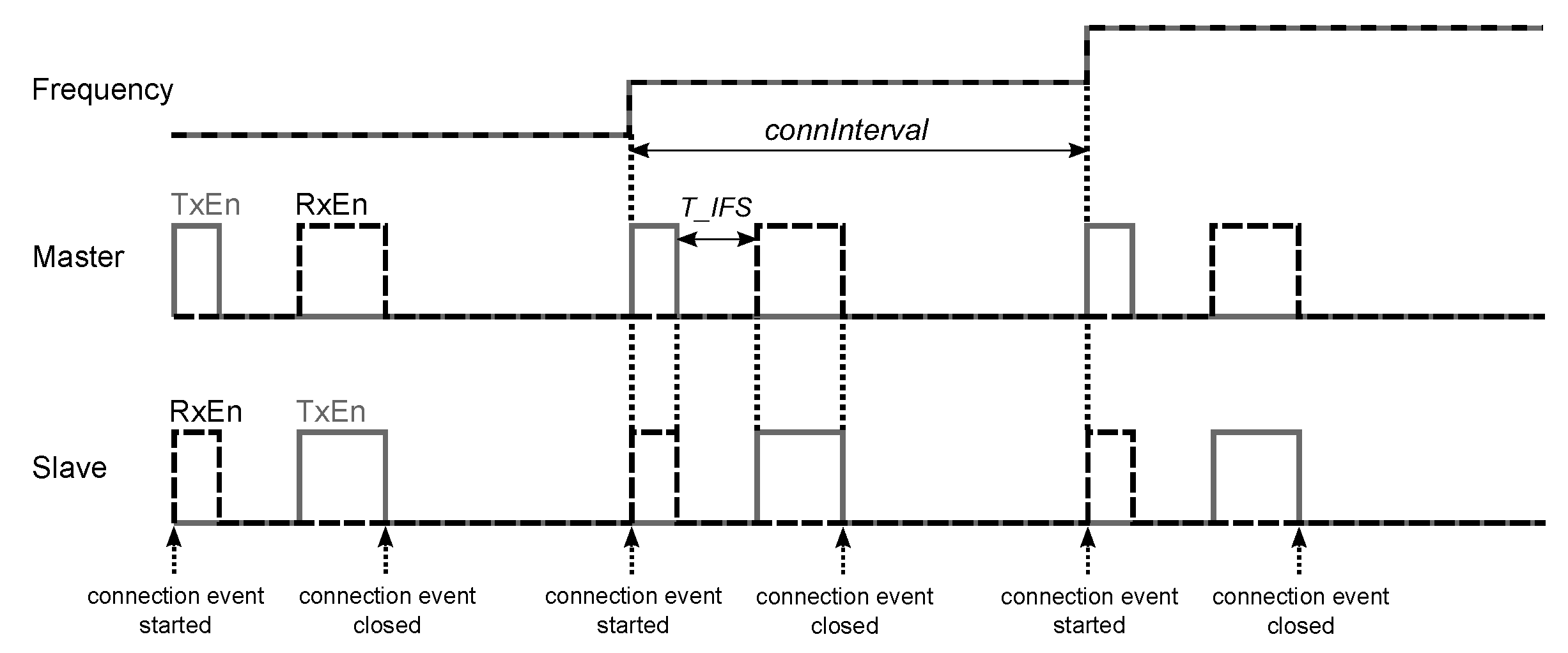
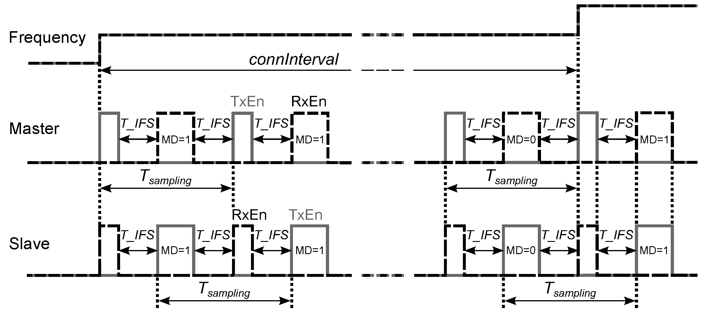
Connection interval—the time interval
between the start of consecutive connection events, which are regularly spaced in time (
Figure 5);
must be a multiple of 1.25 ms in the range from 7.5 ms to 4.0 s ([
24] p. 2980); therefore,
ms, where
is the integer;
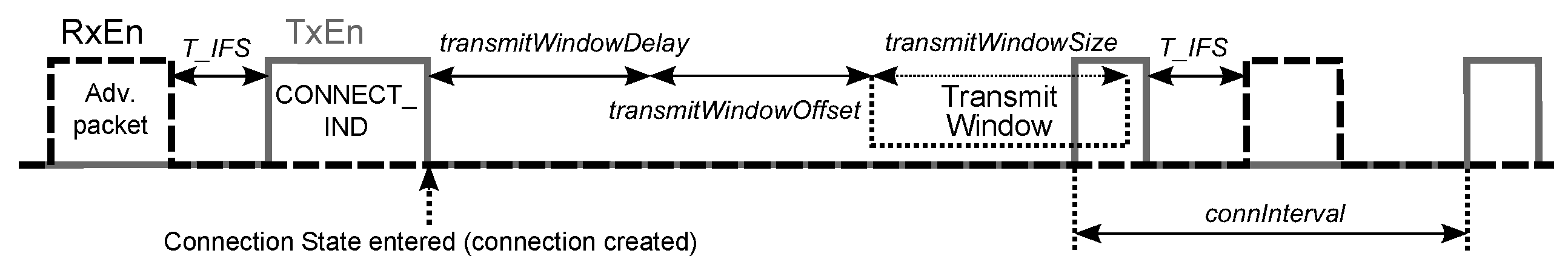
Transmit Window Offset,
Transmit Window Size—the parameters, which determine the anchor point for the first connection event (
Figure 6) and must be multiples of 1.25 ms in the range from 0 ms to
and from 1.25 ms to the lesser of 10 ms and (
ms), respectively ([
24] p. 2983); therefore,
ms and
ms, where
and
are integers;
Connection Supervision Timeout—the maximum time
between two received data packets before the connection is considered lost;
must be a multiple of 10 ms in the range from 100 ms to 32.0 s and larger than
([
24] p. 2981); therefore, given
ms and
, the parameter
ms, where
is the integer;
Connection Slave Latency—the number
of consecutive connection events that the slave is not required to listen for the master;
must be an integer in the range from 0 to
and less than 500 ([
24] p. 2981), which means that
(in the model, this parameter is set to zero; therefore, the slave listens at every anchor point to enable higher sampling rates of the sensors and lower latencies between data acquisition (slave) and data reception (master) sides);
Master SCA—the worst case master’s sleep clock accuracy, which determines the uncertainty window of the slave device at a connection event ([
24] pp. 2883, 2986) (in the model, the sleep clock accuracy is assumed to be 0 ppm, which corresponds to
);
Data acquisition mode:
As follows from the data acquisition mode, master can be set to communicate either with only one slave or with multiple slaves simultaneously—the choice depends on the required sampling frequency of the sensors connected to the slaves. If the sampling rate exceeds 133 Hz, which is the reciprocal of the minimum ms, then only one slave is supported due to continues exchange of the data packets (150 us apart) between the master and the slave. Otherwise, if the sampling rate is no larger than 133 Hz, then only one data packet per connection interval can be received from the slave, granting the master an idle time to communicate with other devices in the time interval between the end of the data packet from the slave and the start of the next connection event.
2.1.1. One Slave Mode
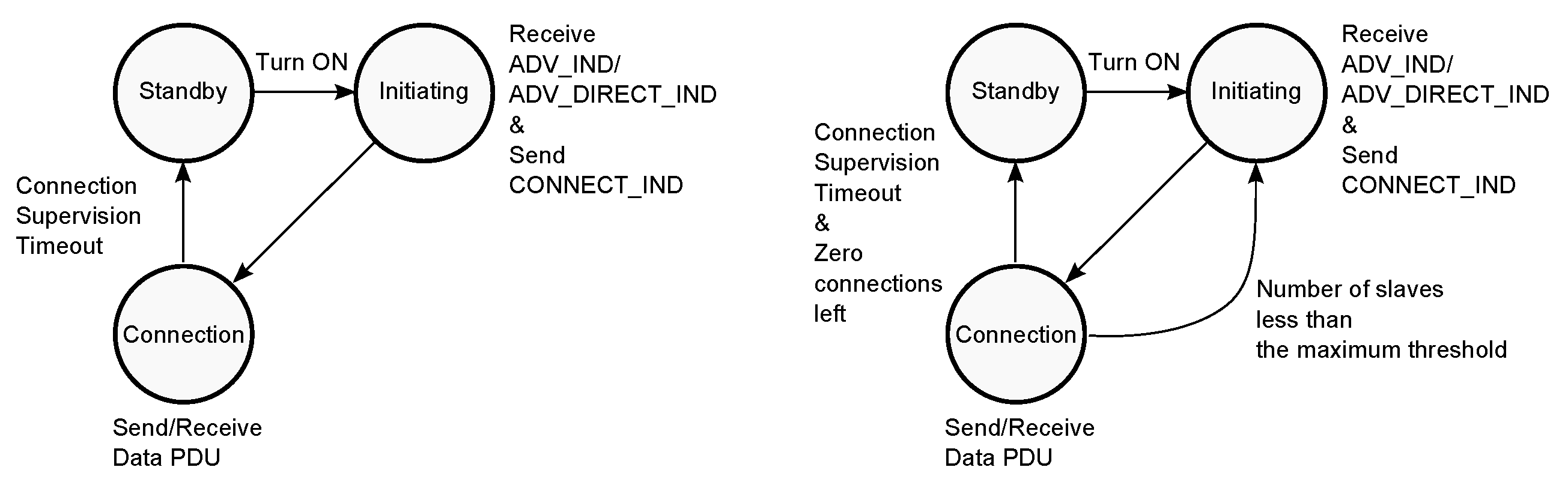
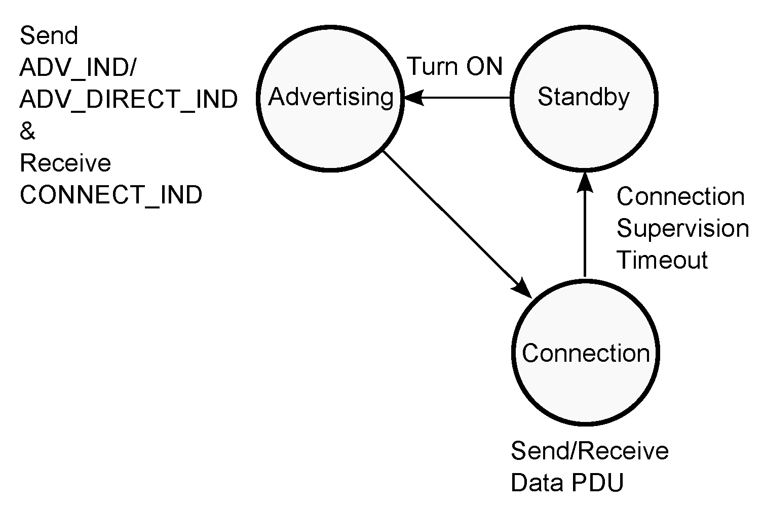
At the start of simulation, the master resides in the Standby State (
Figure 8). At Turn ON time, the master enters the Initiating State and starts to listen on the 3 primary advertising channels for the advertising packets (
Figure 4). If the packet is received, the master sends the initiating packet CONNECT_IND to the slave and transitions to the Connection State. The CONNECT_IND packet contains all the parameters (Access Address, initialization value for the CRC calculation, transmit window size, transmit window offset, connection interval, etc.) that are necessary for establishing the connection between the master and the slave ([
24] p. 2881). In the Connection State, the master sends and receives the data packets to and from the slave. If the connection is lost and the master’s connection supervision timer reaches the Connection Supervision Timeout, the master returns to the Standby State.
2.1.2. Multiple Slaves Mode
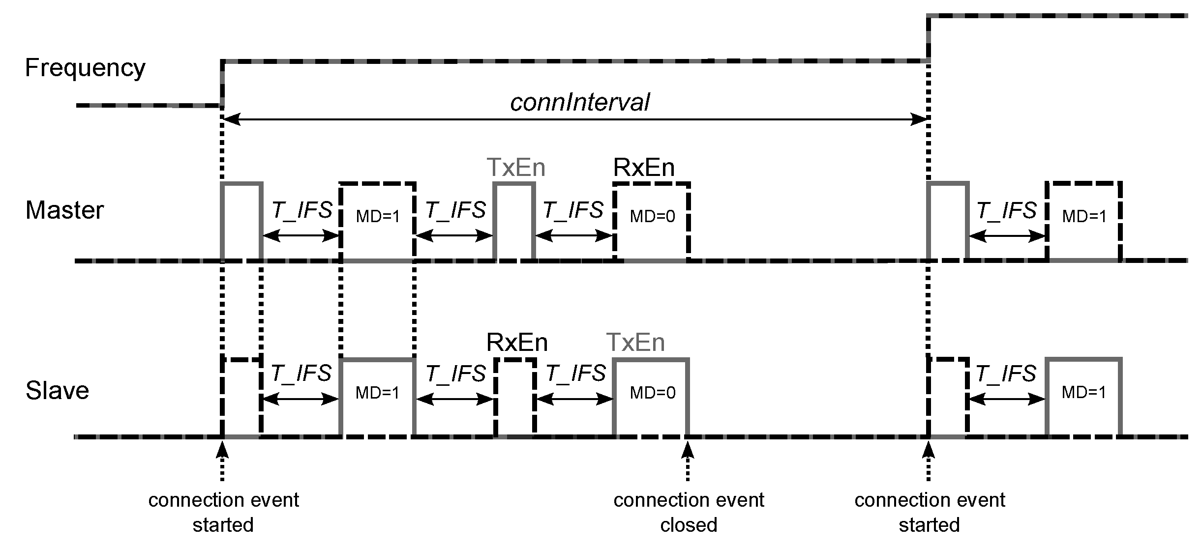
The state diagrams of the master device in one slave and multiple slaves modes are similar (
Figure 8). The difference is that in the latter case the master can return from the Connection State to the Initiating State to listen for new advertisements, while in the former case it is not possible. In the multiple slaves mode, after creating the connection with the first slave, the master subdivides the specified connection interval into 2500 us subintervals, the length of which is determined by the maximum value of the sum
us, where 80 us is the length of the empty data packet sent from the master to the slave, 150 us is the inter frame space succeeding the master’s and the slave’s data packets, and
is the length of the data packet sent from the slave to the master, where
octets is the length of the Paylaod in the slave’s data packet. If
ms is not the multiple of 2.5 ms, then the last subinterval is
ms long, while the rest subintervals are 2.5 ms long.
Each subinterval can be used either for one connection event for sending and receiving one data packet to and from the slave, in which case the master resides in the Connection State, or for listening for new advertisements in the Initiating State (one example is shown in
Figure 9). The master can therefore be in connection with multiple slaves simultaneously, the maximum number of which equals the number of obtained subintervals.
2.2. Slave
The slave (advertiser) block has two inputs and two outputs. The first input is used for connecting the sensors to the slave, while the second input is the received signal from the channel. The first output is the transmitted signal, which goes to the channel, while the second output is the diagnostics bus.
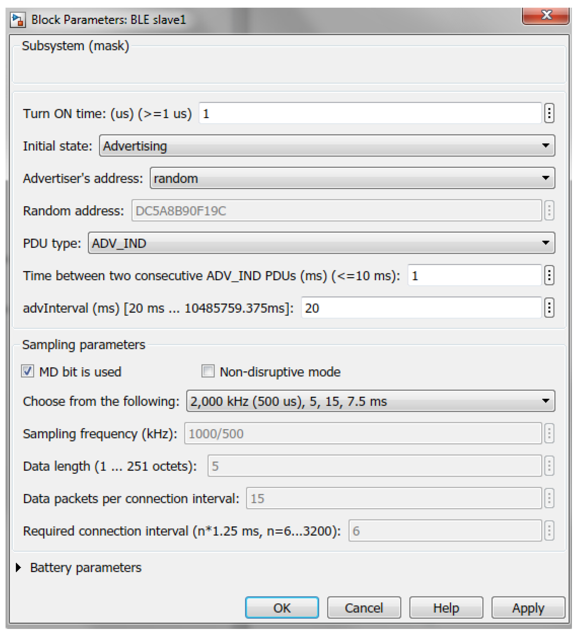
The slave device has the following configurable parameters (
Figure 10).
Turn ON time—indicates, when the device transitions from the Standby State to the Advertising State (all the implemented sates are shown in Figure 13);
Initial state—Advertising State (entered at Turn ON time);
Advertiser’s address—public (manually entered) or random (generated at placing the block in the model) ([
24] p. 2859);
PDU type—advertising PDU ([
24] p. 2873):
ADV_IND has the payload containing only the slave’s address;
ADV_DIRECT_IND has the payload containing the slave’s address and the target’s or master’s address the slave intends to communicate with (by selecting ADV_DIRECT_IND, additional three fields appear in the dialog box, which allow to select the target device from the list of available masters in the model and configure the chosen master by setting its connection interval and data acquisition mode according to the sampling settings required by the slave);
Time between two consecutive ADV_IND PDUs—the time interval
ms between the start of two consecutive advertising packets within an advertising event ([
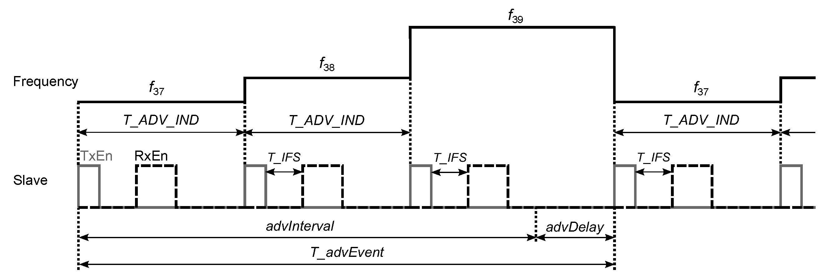
24] p. 2938); the advertising event is composed of three advertising packets sent on 3 primary advertising channels starting from the channel index 37 and ending with the last channel index 39 (
Figure 11); after each advertising packet, the slave listens on the same channel for the initiating packet from the master—if the CONNECT_IND packet is received, the advertising event can be closed early;
advInterval (multiple of 0.625 ms in the range from 20 ms to 10485.759375 ms)—the parameter, which determines the advertising interval
, which is the time between the start of two consecutive advertising events:
, where
ms is a pseudo-random value generated for each advertising event ([
24] p. 2939);
Sampling parameters:
Battery parameters (required for estimating the state of charge of the battery of the slave): battery voltage and capacity; idle state power consumption, when the device is neither transmitting nor receiving; energy spent per bit sent; energy spent per bit received; battery charging power (if zero, the battery is disconnected from the charger).
At the start of simulation, the slave resides in the Standby State (
Figure 13). At Turn ON time, the slave enters the Advertising State and starts to send either ADV_IND or ADV_DIRECT_IND packets on the 3 primary advertising channels (
Figure 11). After sending each packet, the slave listens on the same channel for the initiating packet CONNECT_IND from the master. If the packet is received, the slave transitions to the Connection State, in which it sends and receives the data packets to and from the master. If the connection is lost and the slave’s connection supervision timer reaches the Connection Supervision Timeout, the slave returns to the Standby State.
2.3. Sensor
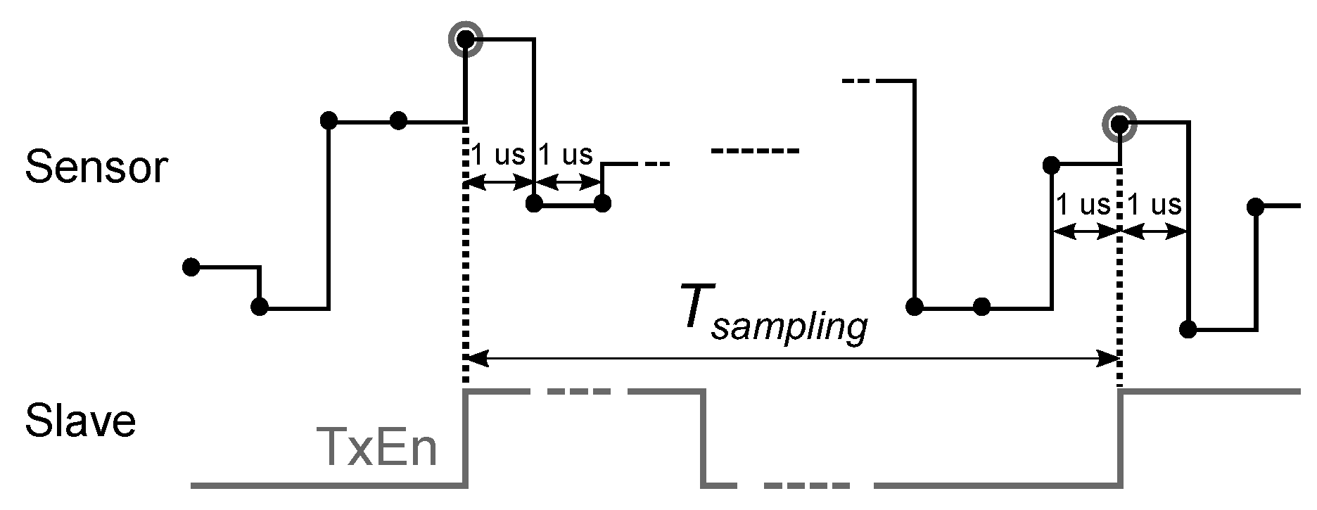
Sensors are simulated as random number generators giving the binary numbers every 1 us in the range from 0 to , where p is the number of bits per sample specified in the dialog box of the sensor block.
When the sensor output is connected to the first input of the slave device, the sensor values are captured by the slave at the rising edges of its transmit enable (TxEn) signal with the periodicity of
(
Figure 14).
2.4. Interferer
The interferer block has two outputs. The first output, which is applied to the channel, provides the signal as specified by IEEE 802.11b standard [
25], while the second output is the diagnostics bus, which contains the transmit enable signal of the device, and the channel frequency index
, which is the integer in the range from 1 to 13 and determines the channel center frequency
Mhz.
For the interferer, the following parameters are configurable:
Average rate—the average number of Poisson-distributed packets per second sent by the interferer;
Mean packet length—the length of the packets sent by the interferer;
Interference frequency number—the channel frequency index used by the interferer.
2.5. Channel
In the library, the channel block has neither inputs nor outputs—the ports appear after creating the model by calling a special function
new_BLE_model (explained in
Section 2.8), which takes into account the number
K of all BLE devices in the model and builds the corresponding internal structure of the block with
inputs and
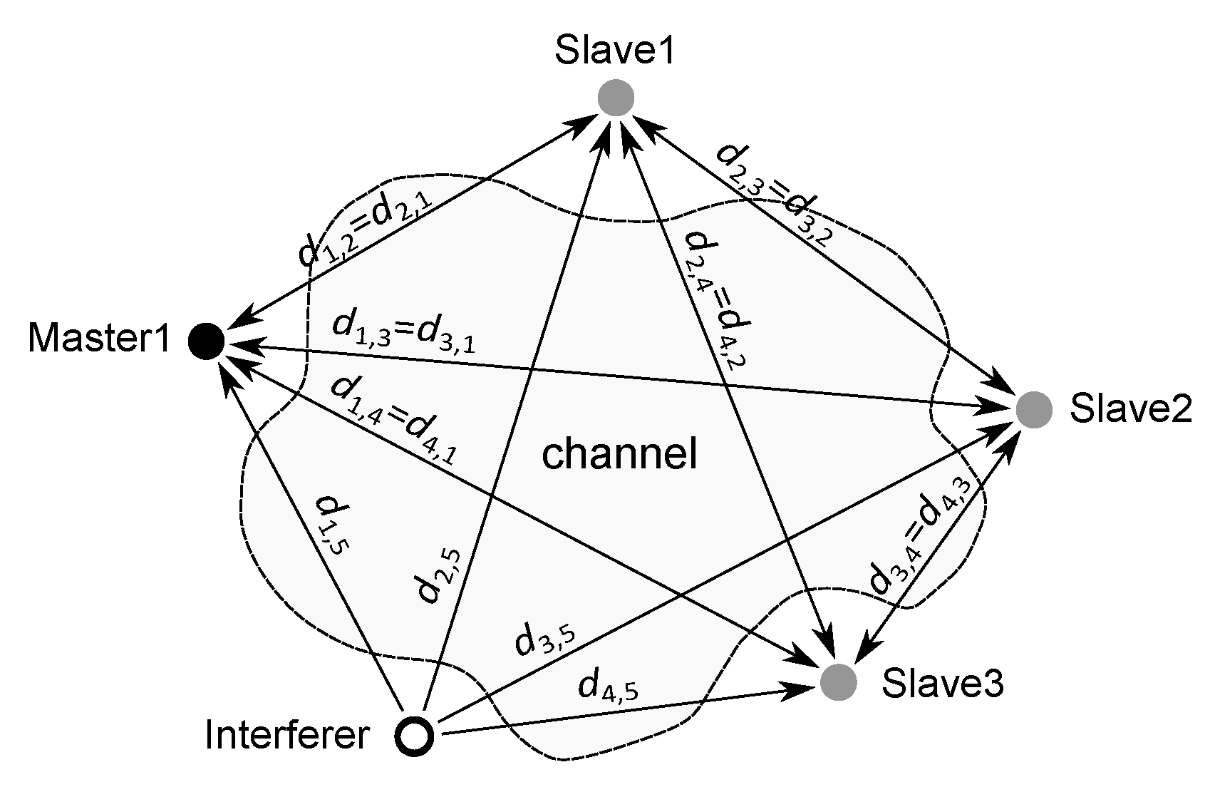
K outputs. The inputs are used for collecting the transmitted signals of the BLE devices and one interferer, while the outputs provide the received signals, which are connected to the inputs of the BLE devices. By denoting the arrays of transmitted and received signals by
and
, respectively, the following equation holds:
where the matrix
contains the attenuation coefficients [
26]
of the transmitted signals depending on the wavelength
m and the distances
between the corresponding devices (
Figure 15), while
is composed of noise signals, which are added to the channel output. When the interferer is disabled, the last column in
, which contains the attenuation coefficients of the interferer signal
, is set to zero.
The following parameters are configurable for the block:
BLE transmit power—the transmission power level, which is equal for all BLE devices in the model (can be varied individually after the model has been created);
AWGN channel noise power—the additive white Gaussian noise power, which is also equal for all BLE devices and can be varied individually after creating the model;
Interferer On—enable or disable the 802.11b interference signal;
Interferer transmit power—the transmission power level of the 802.11b interferer.
2.6. Diagnostics
The diagnostics block allows to observe the quality of communication between one selected slave device and one master. It also contains one scope showing different internal signals of the devices during the simulation.
The block has three inputs and four outputs. The inputs are connected to the diagnostics buses of one slave, one master and the interferer, while the first three outputs provide the Bit Error Rate (BER—the number of bit errors divided by the total number of transferred bits), the Packet Error Rate (PER—the number of invalid packets divided by the total number of valid packets) and the Packet Rejection Rate (PRR—number of rejected packets divided by the total number of transferred packets) of the packets sent from the slave to the master. The last output gives the battery status of the slave, which indicates both the state of charge (SOC) and the time left to fully charge or discharge the battery.
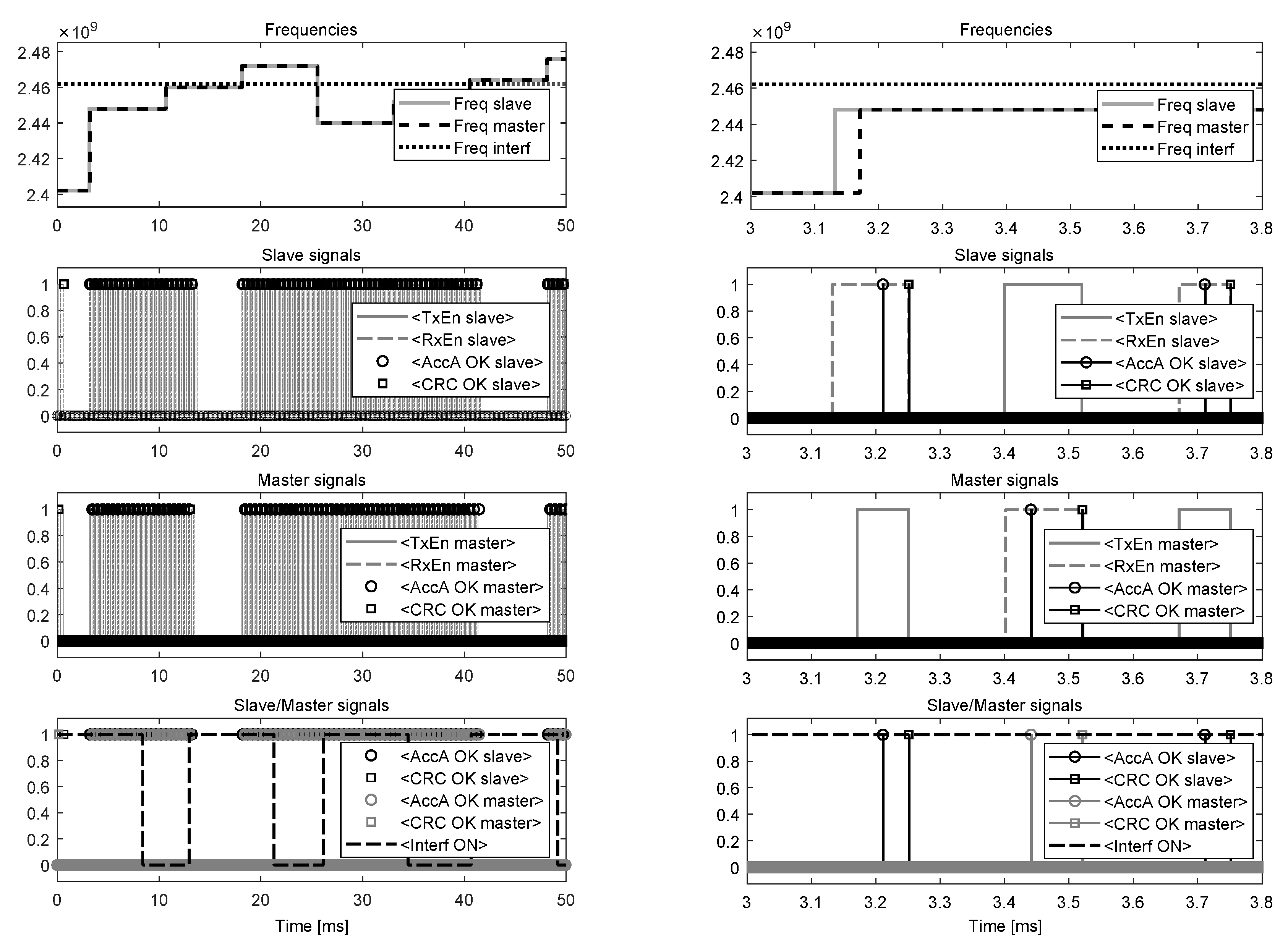
When the simulation starts, the built-in scope of the diagnostics block opens four displays showing: (1) channel frequencies used by the selected slave and the master, and the interferer; (2) transmit enable (TxEn), receive enable (RxEn), Access Address control (AccA OK) and CRC control (CRC OK) signals of the slave (AccA OK and CRC OK signals are composed of 1 us pulses, which are generated after verifying the correctness of the Access Address and CRC fields of the received packets, respectively); (3) TxEn, RxEn, AccA OK and CRC OK signals of the master; (4) AccA OK and CRC OK signals of the slave and the master, and the control signal (InterfON) of the interferer, which shows when the device is transmitting to see its impact on data exchange between the chosen two BLE devices (the example in Figure 17 shows that when the interferer is turned on and its channel frequency is close to the frequency of the master and the slave, the connection events disrupt due to either not receiving the packets (Access Address is incorrect) or receiving two consecutive packets with invalid CRC match).
2.7. Exporting
The library contains the block for exporting the settings of the BLE devices. After placing the block in the model and by double clicking on its icon, the parameters of the devices are stored in plain text files, which can be used for identical configuration of real-world devices.
2.8. Creating the Model
For creating the initial BLE models, a special MATLAB function
can be used, which allows to specify the locations of the devices (the Cartesian coordinates
x and
y of the master devices, slaves and the interferer are given by
xy_M,
xy_S and
xy_I, respectively) to take into account the distances between them (the distances are used for calculating the attenuation matrix
in the channel block). In addition, the devices in the model are placed in accordance to their given locations with the scale of the model saved in the model workspace (the scale of the model is the ratio of a distance in the model to the corresponding real distance following from the given coordinates). Every time the simulation starts, the distances and the matrix
are recalculated; therefore, after the model has been created, the locations of the devices can be changed as necessary.
When placing additional BLE devices in the model after the model has been created, the channel block should be changed accordingly with its inputs connected to the outputs of the master devices, slaves and the interferer, while the outputs of the channel block should be connected to the corresponding inputs of the masters, then slaves.
In the Simulink, by opening the Diagnostic Viewer, the messages generated by the devices during the simulation can be observed. For the master device, the messages are produced when the master: (1) enters the Initiating State; (2) receives the advertising packet from the slave; (3) creates the connection with the slave; (4) sets the anchor point for the connection; (5) establishes the connection with the slave; (6) checks the CRC validity of the received packet; (7) terminates the connection with the slave. Similarly, for the slave device, the messages are produced when the slave: (1) enters the Advertising State; (2) starts or closes the advertising event; (3) creates the connection with the master; (4) establishes or fails to establish the anchor point for the connection; (5) establishes the connection with the master; (6) checks the CRC validity of the received packet; (7) terminates the connection with the master. For correctly displaying the messages in the Diagnostic Viewer, the names to the BLE devices should be given as ‘BLE masterX’ or ‘BLE slaveY’, where X and Y are integer numbers.
3. Simulation Examples
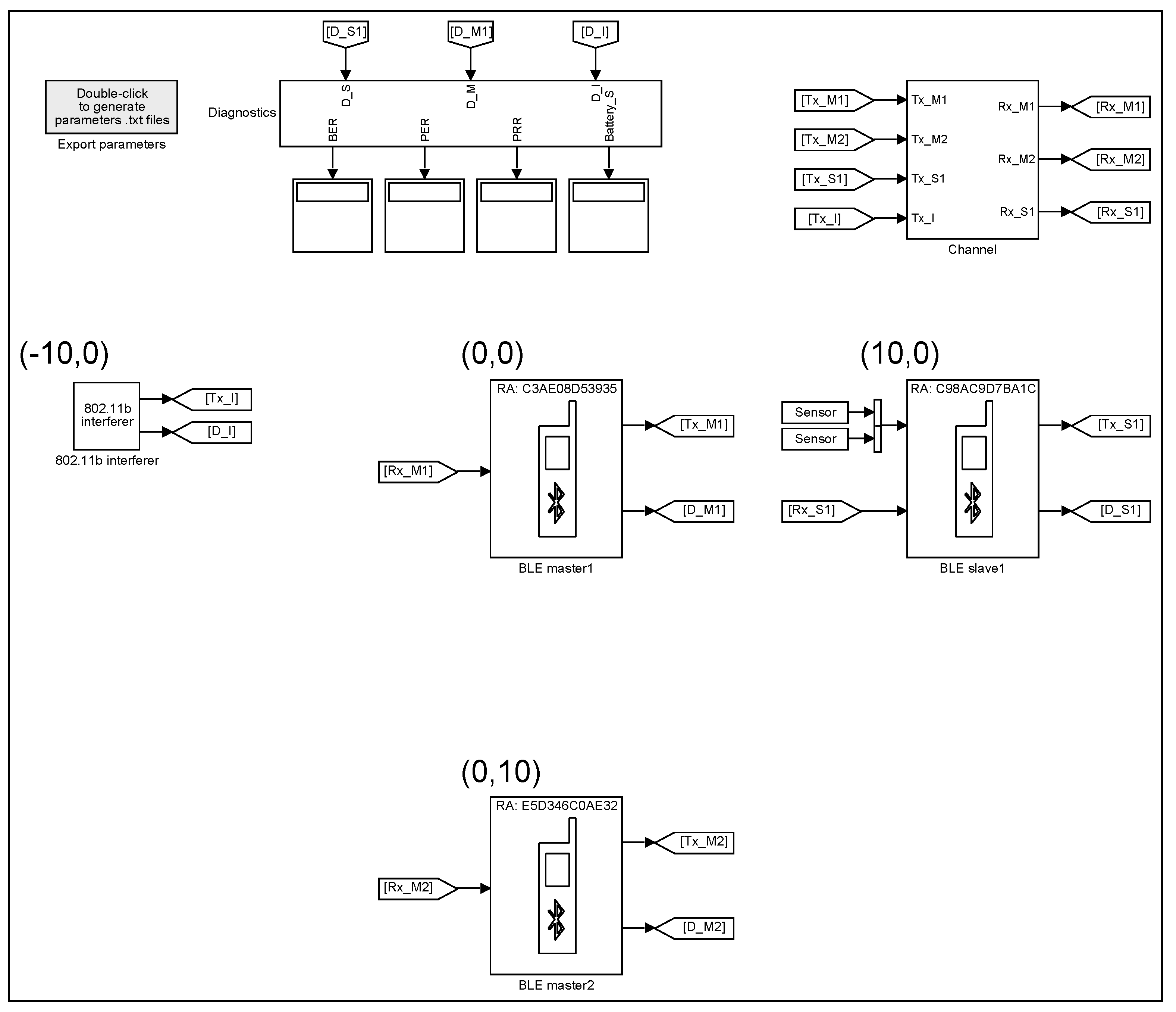
Example 1. By calling the function
new_BLE_model(M2S1, [0,0; 0,10], [10,0], [−10,0]), the model in
Figure 16 is created. The model contains two master devices and one slave, which means that both the masters will respond to the advertising packet ADV_IND sent by the slave causing the interference between the packets; therefore, depending on the signal strength, the connection may be established with only either master1 or master2. The addresses of the BLE devices are random and shown on their icons, while their configurations conform to the dialog boxes in
Figure 3 and
Figure 10, respectively. The interferer’s parameters (Average rate, Mean packet length, Interference frequency number) are set to 70 packets per second, 8384 bits per packet and 11, respectively, while the channel’s parameters (BLE transmit power, AWGN channel noise power, Interferer On, Interferer frequency number) are 0 dBm, −80 dBm, enabled and 0 dBm, respectively. After running the simulation for 50 ms, the signals displayed by the scope of the diagnostics block are shown in
Figure 17, while the messages appearing in the Diagnostic Viewer are as follows:
M1: initiating state entered at 0.000 ms
M2: initiating state entered at 0.000 ms
S1: advertising state entered at 0.001 ms
S1: advertising event started at 0.001 ms
M1: advertising packet received from S1 at 0.130 ms
M2: advertising packet received from S1 at 0.130 ms
M1: connection created with S1 at 0.632 ms
S1: connection created with M1 at 0.632 ms
M2: connection created with S1 at 0.632 ms
M1: anchor point set for S1 at 3.171 ms
M2: anchor point set for S1 at 3.191 ms
S1: anchor point established for M1 at 3.171 ms
S1: connection established with M1 at 3.251 ms
S1: CRC passed from M1 at 3.251 ms
M2: CRC failed from S1 at 3.501 ms
M1: connection established with S1 at 3.521 ms
M1: CRC passed from S1 at 3.521 ms
S1: CRC passed from M1 at 3.751 ms
M1: CRC passed from S1 at 4.021 ms
S1: CRC passed from M1 at 4.251 ms
M2: CRC failed from S1 at 11.001 ms
M1: CRC passed from S1 at 13.021 ms
S1: CRC passed from M1 at 13.251 ms
M1: CRC failed from S1 at 13.521 ms
S1: CRC failed from M1 at 13.751 ms
S1: CRC passed from M1 at 18.251 ms
M2: CRC failed from S1 at 18.501 ms
M1: CRC passed from S1 at 18.521 ms
S1: CRC passed from M1 at 18.751 ms
M2: CRC failed from S1 at 26.001 ms
M2: CRC failed from S1 at 33.501 ms
M1: CRC passed from S1 at 40.521 ms
S1: CRC passed from M1 at 40.751 ms
M2: CRC failed from S1 at 41.001 ms
M1: CRC failed from S1 at 41.021 ms
S1: CRC passed from M1 at 41.251 ms
M1: CRC failed from S1 at 41.521 ms
S1: CRC failed from M1 at 41.751 ms
M2: connection terminated with S1 at 45.632 ms
S1: CRC passed from M1 at 48.251 ms
M1: CRC passed from S1 at 48.521 ms
S1: CRC passed from M1 at 48.751 ms
⋮
At the start of simulation, both the masters (M1 and M2) enter the Initiating State and receive the advertising packet from the slave (S1) at 0.13 ms. After
ms, each master starts sending the CONNECT_IND packet to S1 and enters the Connection State (creates the connection with S1) after the packet has been sent at
ms, where 0.352 ms is the length of the CONNECT_IND packet, and, depending on the parameters
and
indicated in the CONNECT_IND packet, calculates the anchor point (
ms and
ms are obtained by M1 and M2, respectively) for the new connection. At the same moment (at 0.632 ms), S1 successfully receives the initiating packet from M1 (located closer to S1) and creates the connection with it. Given the already calculated anchor points, M1 and M2 start to send their empty data channel packets of length 0.08 ms to S1 at
and
, respectively, while S1 receives the data packet (and checks its CRC) only from M1 at
ms (after confirming the correctness of the Access Address of the packet, S1 determines the anchor point for the connection and establishes the connection with M1 after receiving the whole packet at 3.251 ms). In response to the data packet from M1, the slave sends its data packet with the MD bit set to 1 (according to the sampling parameters in
Figure 10) to M1, which receives the packet and establishes the connection with S1 at
ms, where 0.12 ms is the length of the data packet from S1, while M2 fails (due to S1 has not created the connection with M2) to receive the data packets from S1 at
ms (
) until the connection is terminated at
ms, where
, and
ms. Exchange of the data packets between M1 and S1 continues with periodicity of 0.5 ms and stops shortly after the interferer starts to transmit at 12.962 ms and 40.834 ms, and its channel frequency is close to the frequencies used by M1 and S1 (shown in
Figure 17 on the left). The data exchange between M1 and S1 restarts at the beginning of the new connection events at 18.171 ms and 48.171 ms, respectively, when the channel frequencies of M1 and S1 hop to other values more distant from the interferer’s frequency.
If the coordinates of M1 are changed to (−6,0), then S1 creates and establishes the connection with M2, which is now closer to S1, however, if the PDU type in
Figure 10 is changed to ADV_DIRECT_IND with M1 indicated as the target device, then S1 creates and establishes the connection with M1.
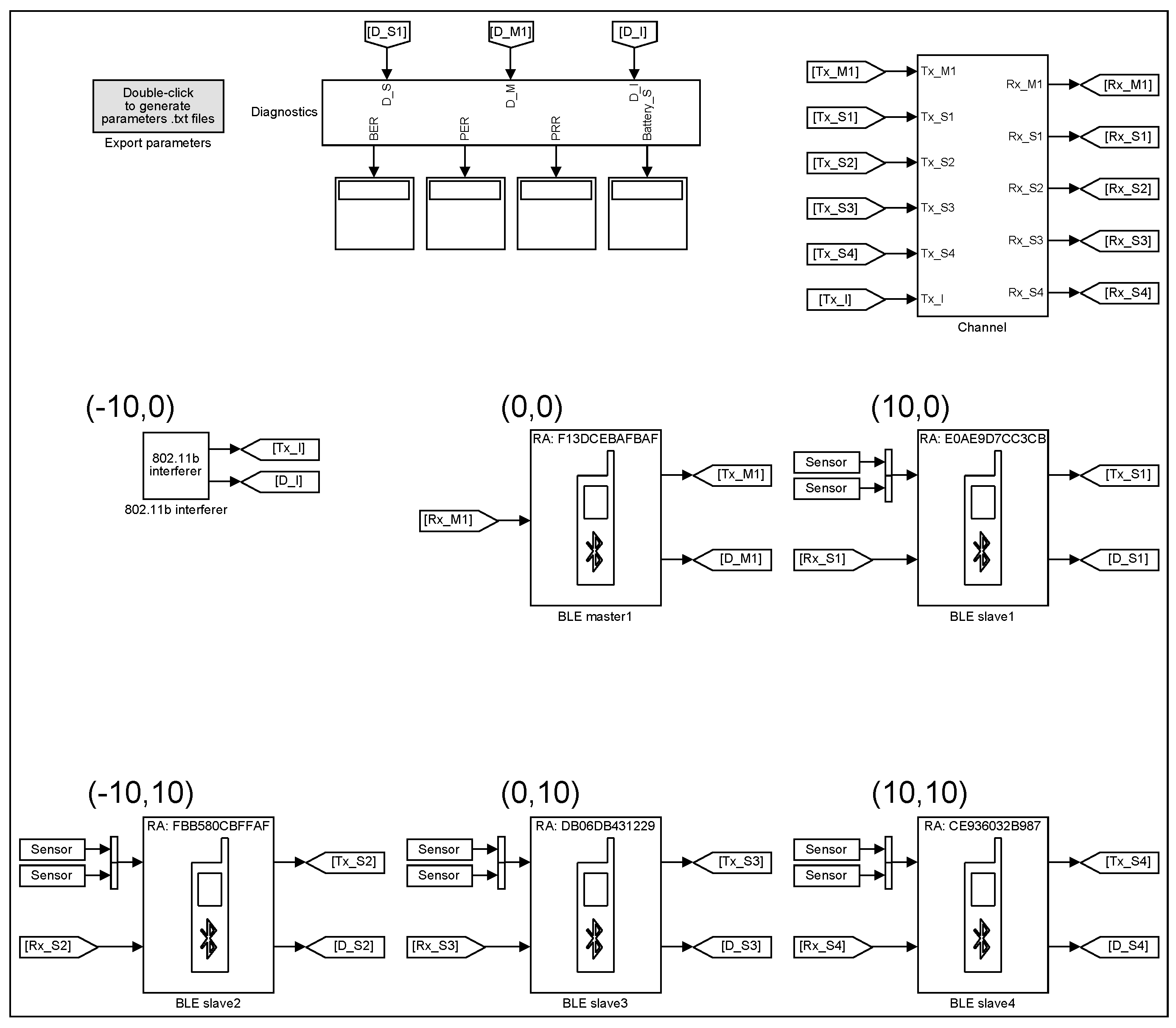
Example 2. By calling the function
new_BLE_model(M1S4, [0,0], [10,0; −10,10; 0,10; 10,10], [−10,0]), the model in
Figure 18 is created. The master device (M1) is configured as in
Figure 3 with the data acquisition mode selected: MD bit is ignored (supports multiple slaves); while the slaves (S1, S2, S3 and S4) have their configurations as in
Figure 10 with Turn ON times: 1 us, 15 ms, 1 ms and 110 ms, respectively; sampling parameters: MD bit is not used; data lengths:
,
,
and
octets, respectively. In addition, the input and output RF signals of S1 are disabled at 11 ms to simulate the link loss between S1 and M1. The parameters of the channel block (BLE transmit power, AWGN channel noise power, Interferer On, Interferer frequency number) are 0 dBm, −80 dBm, disabled and 0 dBm, respectively. After running the simulation for 120 ms, the messages from the Diagnostic Viewer are as follows:
M1: initiating state entered at 0.000 ms
S1: advertising state entered at 0.001 ms
S1: advertising event started at 0.001 ms
M1: advertising packet received from S1 at 0.130 ms
M1: connection created with S1 at 0.632 ms
M1: anchor point set for S1 at 4.284 ms
S1: connection created with M1 at 0.632 ms
M1: initiating state entered at 0.782 ms
S3: advertising state entered at 1.000 ms
S3: advertising event started at 1.000 ms
M1: advertising packet received from S3 at 1.129 ms
M1: connection created with S3 at 1.631 ms
M1: anchor point set for S3 at 6.784 ms
S3: connection created with M1 at 1.631 ms
M1: initiating state entered at 1.781 ms
S1: anchor point established for M1 at 4.284 ms
S1: connection established with M1 at 4.364 ms
S1: CRC passed from M1 at 4.364 ms
M1: connection established with S1 at 4.914 ms
M1: CRC passed from S1 at 4.914 ms
S3: anchor point established for M1 at 6.784 ms
S3: connection established with M1 at 6.864 ms
S3: CRC passed from M1 at 6.864 ms
M1: connection established with S3 at 8.094 ms
M1: CRC passed from S3 at 8.094 ms
M1: initiating state entered at 9.284 ms
S1: CRC failed from M1 at 11.864 ms
M1: CRC failed from S1 at 13.094 ms
S3: CRC passed from M1 at 14.364 ms
S2: advertising state entered at 15.000 ms
S2: advertising event started at 15.000 ms
M1: CRC passed from S3 at 15.594 ms
M1: initiating state entered at 16.784 ms
M1: advertising packet received from S2 at 17.129 ms
M1: connection created with S2 at 17.631 ms
M1: anchor point set for S2 at 24.284 ms
S2: connection created with M1 at 17.631 ms
S1: CRC failed from M1 at 19.364 ms
M1: CRC failed from S1 at 20.594 ms
S3: CRC passed from M1 at 21.864 ms
M1: CRC passed from S3 at 23.094 ms
S2: anchor point established for M1 at 24.284 ms
S2: connection established with M1 at 24.364 ms
S2: CRC passed from M1 at 24.364 ms
M1: connection established with S2 at 26.602 ms
M1: CRC passed from S2 at 26.602 ms
S1: CRC failed from M1 at 26.864 ms
M1: CRC failed from S1 at 29.102 ms
S3: CRC passed from M1 at 29.364 ms
⋮
S3: CRC passed from M1 at 96.864 ms
M1: CRC passed from S3 at 98.094 ms
S2: CRC passed from M1 at 99.364 ms
M1: CRC passed from S2 at 101.602 ms
S1: CRC failed from M1 at 101.864 ms
M1: CRC failed from S1 at 104.102 ms
S1: connection terminated with M1 at 104.364 ms
S3: CRC passed from M1 at 104.364 ms
M1: connection terminated with S1 at 104.914 ms
M1: CRC passed from S3 at 105.594 ms
S2: CRC passed from M1 at 106.864 ms
M1: CRC passed from S2 at 109.102 ms
M1: initiating state entered at 109.284 ms
S4: advertising state entered at 110.000 ms
S4: advertising event started at 110.000 ms
M1: advertising packet received from S4 at 110.129 ms
M1: connection created with S4 at 110.631 ms
M1: anchor point set for S4 at 116.784 ms
S4: connection created with M1 at 110.631 ms
S3: CRC passed from M1 at 111.864 ms
M1: CRC passed from S3 at 113.094 ms
S2: CRC passed from M1 at 114.364 ms
M1: CRC passed from S2 at 116.602 ms
S4: anchor point established for M1 at 116.784 ms
S4: connection established with M1 at 116.864 ms
S4: CRC passed from M1 at 116.864 ms
M1: connection established with S4 at 117.134 ms
M1: CRC passed from S4 at 117.134 ms
S3: CRC passed from M1 at 119.364 ms
⋮
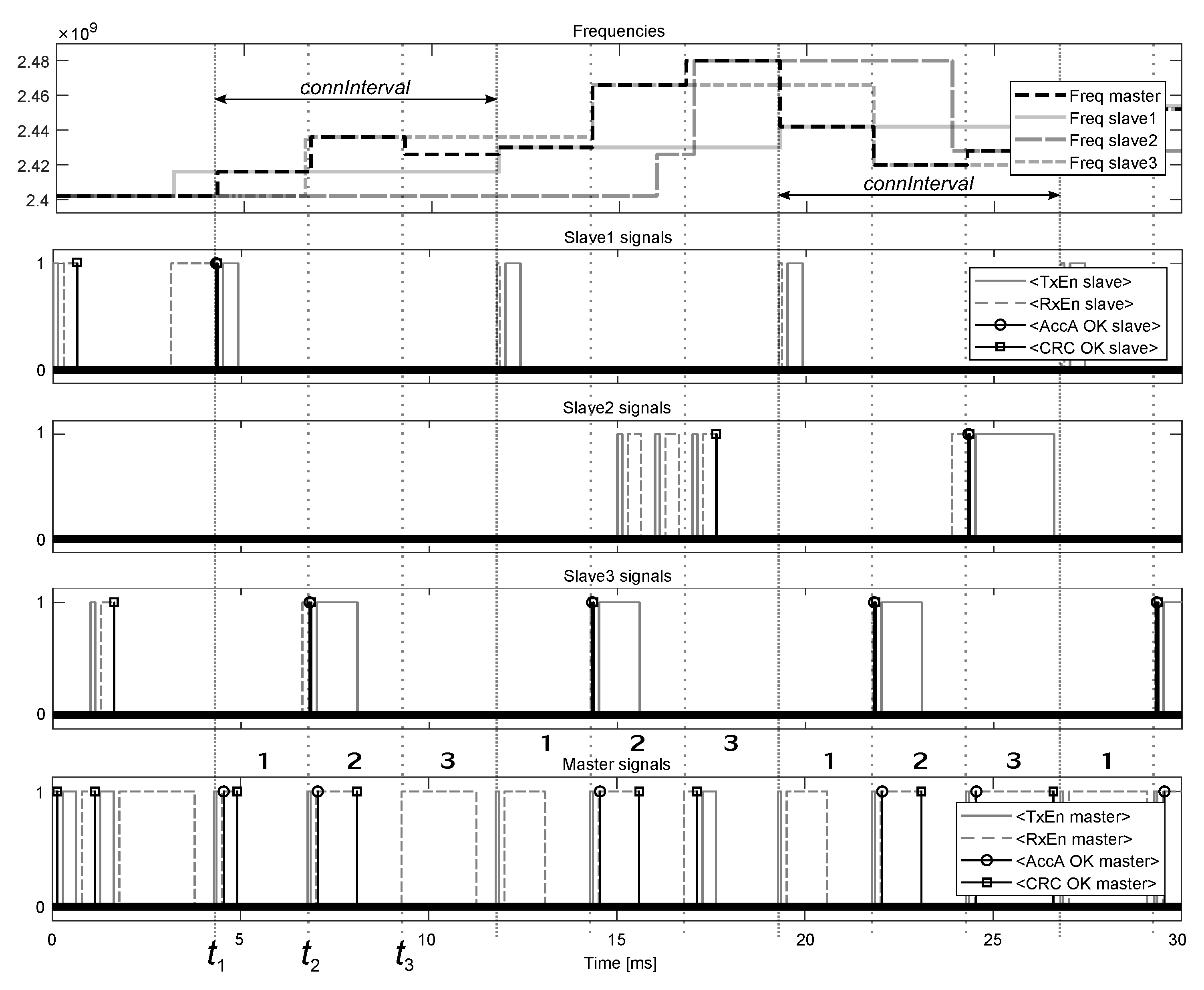
At the start of simulation, M1 enters the Initiating State and receives the advertising packet from S1 at 0.130 ms. M1 responds to the packet by sending the initiating packet with the indicated
ms to S1 and creates the connection with the slave at 0.632 ms. At this moment, the anchor point for the connection is set to
ms, and M1 returns to the Initiating State at
ms for listening for new advertisements from other devices. At 1.129 ms, M1 receives the advertising packet from S3, which is responded by sending the initiating packet to S3 and creating the connection with the slave at 1.631 ms. The anchor point for this connection is set to
ms, where 2.5 ms is the length of the subinterval in the multiple slaves mode (in total, there are
2.5
3 subintervals). M1 returns to the Initiating State at
ms but receives no new advertisements up to
ms, where
ms is the time interval reserved for responding with the initiating packet of length 0.352 ms to an advertiser and entering the Connection State. At
, which is the start of the first subinterval (
Figure 19), M1 begins to send the empty data packet of length 0.08 ms to S1, which receives the packet and establishes the connection with M1 at
ms, while M1 receives the data packet and establishes the connection with S1 at
ms, where
ms is the length of the data packet from S1. Similarly, at
, which is the start of the second subinterval, M1 begins sending the data packet to S3, which receives the packet and establishes the connection with M1 at
ms, while M1 establishes the connection with S3 after receiving the data packet from the slave at
ms. Whereas at
ms, which is the start of the third subinterval, M1 enters the Initiating State and listens for new advertisements until
.
At
(
), which are the starting points of the first subintervals, M1 begins to send the data packets to S1 but receives no responses; therefore, M1 terminates the connection with S1 at
ms, where 4.914 ms is the moment of receiving the last data packet from S1, while
ms, as indicated in
Figure 3, whereas S1 terminates the connection with M1 at
ms. After termination, M1 uses the first subintervals for listening for new advertisements, and receives the advertising packet from S4 at 110.129 ms, which is followed by creating and establishing the connection with the slave at 110.631 ms and 117.134 ms, respectively.
At , which are the starting points of the second subintervals, M1 begins to send the data packets to S3, which are received by the slave at ms, while the responding packets from S3 are received by M1 at ms.
In the third subintervals, which start at , M1 resides in the Initiating State until the advertising packet from S2 is received at 17.129 ms. After creating and establishing the connection with S2 at 17.631 ms and 26.602 ms, respectively, the third subintervals are used for exchanging the data packets between M1 and S2.
4. Conclusions
The developed library allows to build different models of BLE wireless sensor networks for testing the communication between multiple BLE devices in the presence of interference and channel noise. The number of devices, which can be placed in a model, are theoretically unlimited, however, in practice, a restrictive factor is the processing power of a computing machine. For example, the models
M2S1 and
M1S4 in
Section 3 required 0.5 s and 1.33 s, respectively, of computing time (Intel (R) Core (TM) i5-3470 CPU, RAM of 16 GB) to calculate 1 ms of the simulation time.
The master and slave blocks operate as specified by the BLE protocol, however, not all features are implemented: (1) in the models, the clocks of the devices are assumed to be precise; therefore, window widening ([
24] p. 2930) is not implemented, which also means that signal delays due to propagation through the channel are not taken into account; (2) the channel map in channel selection algorithm ([
24] p. 2987) is not updated during the simulation by assuming that all 37 data channels are constantly available for data transmission; (3) the acknowledgment and flow control scheme ([
24] p. 2995) is not fully implemented because of the requirement for high sampling rates (at least 1.6 kHz) of the sensors and low latencies (under 500 us) for data transmission, which means that resending of unacknowledged data packets is not possible (for the same reason, the connection slave latency in
Figure 3 can not exceed 0). In addition, the Scanning State for the BLE devices is not implemented due to not suiting the purpose of simulating the data exchange at high packet transmission rates, which can reach up to 2137 packets per second as follows from
Table 1.


