Article

Noise Reduction Scheme for Parametric Loop Division 3D Wireless Localization Algorithm Based on Extended Kalman Filtering

Department of Electrical and Electronic Engineering, Auckland University of Technology, Auckland 1010, New Zealand
*
Author to whom correspondence should be addressed.
J. Sens. Actuator Netw. 2019, 8(2), 24; https://doi.org/10.3390/jsan8020024
Submission received: 17 March 2019 / Revised: 15 April 2019 / Accepted: 24 April 2019 / Published: 28 April 2019

Abstract

:
Thanks to IEEE 802.15.4 defining the operation of low-rate wireless personal area networks (LR-WPANs), the door is open for localizing sensor nodes using tiny, low power digital radios such as Zigbee. In this paper, we propose a three-dimensional (3D) localization scheme based on well-known loop invariant for division algorithm. Parametric points are proposed by using the reference anchor points bounded in an outer region named as Parametric Loop Division (PLD) algorithm. Similar to other range-based localization methods, PLD is often influenced by measurement noise which greatly degrades the performance of PLD algorithm. We propose to adopt extended Kalman filtering (EKF) to refine node coordinates to mitigate the measurement noise. We provide an analytical framework for the proposed scheme and find the lower bound for its localization accuracy. Simulation results show that compared with the existing PLD algorithm, our technique always achieves better positioning accuracy regardless of network topology, communication radius, noise statistics, and the node degree of the network. The proposed scheme PLD-EKF provides an average localization accuracy of 0.42 m with a standard deviation of 0.26 m.

1. Introduction

Advancement in wireless communication technologies and electronic systems leads to the implementation of wireless sensor networks (WSN) which plays an important role in Internet of Things (IoT). A WSN consists of several nodes, which possess low power and low cost devices armed with a processor, one or more sensors, a power [1]. The feasibility of WSNs cost-effective deployment in an open environment made this technology promising for different applications such as surveillance, home automation, human interfacing and cattle farming [2]. Consequently, sensor localization is necessary for those location aware applications, which can analyze data based on physical location. It is therefore necessary to estimate the each sensor location in a WSN after deployment. The most popular wireless localization technology is global positioning system (GPS). However, practically it is hard to use GPS due to the following factors: (1) line of sight between a sensor node and GPS satellites is not always available. For instance, it does not work indoor, under water or in a subway. (2) high energy consumption and cost makes it impossible to equip each sensor node with GPS modules. (3) finally sensors are usually designed for low power consumption but GPS receivers are highly power consuming.
The developed localization methods can be classified into two categories: range-based and range-free algorithms [3] as shown in Figure 1. Distance or angle between the unknown nodes and the sink node can be determined in range-based techniques, while range-free solutions achieved through radio connectivity that exploits the sensing capabilities of each sensor. Range-based localization system first estimate distance using different methods such as Time of Arrival (ToA) [4], Time Difference of Arrival (TDoA) [5], Angle of Arrival (AoA) [6], and others based on Received signal strength indicator (RSSI) [7,8,9,10,11]. Location estimation can adopt triangulation localization algorithms, trilateration localization methods or maximum likelihood estimation methods presented in different articles [12,13]. Range-free approaches simply use sensing features such as wireless connectivity, localization event detection and beacon/anchor node proximity [14,15], resulting in a low cost solution at the expense of localization accuracy. In particular radio frequency (RF) signals are sensitive to environment environmental impact, leading to instability of RSSI [16].
Fingerprinting-based localization will be in two phases. In first phase, also known as online phase, a database of the RSS from different access points at each reference location for the target environment is built. In second phase (offline phase), by means of a sample RSS collected at a particular node and an estimation algorithm with the RSSI database, the node location is determined. In this group, several different techniques and approaches, such as the ray tracing model [17], support vector machine [18], data mining techniques [19], probabilistic methods [20], and some others based on Kalman filtering [21] were reported. Most works focus on two dimensional (2D) localization. This motivated us to propose a three-dimensional (3D) localization scheme based on parametric loop division (PLD) [3], to improve localization accuracy, minimize the computational load and mitigate the dependence of anchor node deployment. Loop subdivision algorithm is widely used for its simple rules, excellent continuity, and its triangular controllable meshes [22]. In this paper, we extend our proposed PLD scheme to enhance its noise awareness through extended Kalman filtering technique. The rest of the paper is organized as follows. Section 2 presents the related work in the field. Section 3 describes the main functionality of noise aware PLD algorithm by describing the key idea, PLD algorithm steps with and without implementing noise and use of extended Kalman filtering on the coordinates of PLD to get the refine coordinates. Section 4 presents simulation results and discussion on the effect of using EKF for noise suppression. Finally, Section 5 concludes the paper with future work.

2. Related Work

Short range wireless communication-based technologies that can consider for WSN are RFID, Zigbee, and Bluetooth etc. ZigBee is a low power consumption, low cost, low data rate and large network capacity communication protocol based on IEEE 802.15.4 standard [23]. Wireless sensor networks using ZigBee are employed in a wide number of applications such as device tracking, habitat monitoring, agriculture and smart homes. The closely related WirelessHART and 6LoWPAN, based on the same radio standard, are increasingly used for wireless machine-to-machine (M2M) communication and office automation. Several techniques have been proposed in the literature for estimating the position of sensor nodes in sensor networks. Range-free localization schemes such as centroid localization [24], have much attraction due to simplicity and robustness to changes in wireless propagation properties such as path loss. The idea of 3D localization based on social network analysis also getting much attraction due to its simplicity and use of closeness centrality value as a metric of weight [25].
Ad-hoc positioning system (APS) proposed in [14], multilateration was not possible because of sensor node deployment structure. No node in a network receive beacon from at least three anchors so they do not form a triangle for localizing the node. APS system used hybrid-based methods combining distance vector like propagation and GPS triangulations. This system is a distributed system and therefore does not require any special infrastructure for node deployment.
The multi-dimensional scaling (MDS)-based algorithm was proposed in [26]. MDS was from mathematical psychology, which provides a method to display the structure of distance-link data as a geometrical picture. The proposed MDS-MAP scheme had three steps: (1) Estimation of distance between each possible pair of nodes; (2) Derivation of node localization using MDS to fit those estimated distances; (3) Normalization of the resulting coordinates using known information of anchor nodes. MDS-MAP could generate a relative map of nodes without any anchor node. With three or more anchor nodes, the absolute coordinates of nodes can be estimated.
The APIT technique proposed in was based on Point-in-Triangle Test (PIT) [24], under which a target node chooses three beacon nodes and then tests whether it is inside the triangle or not by connecting three beacon nodes. The APIT algorithm has four steps: (1) Reference exchange; (2) PIT Test; (3) APIT aggregation; and (4) Centre of gravity Calculation (centroid localization). Simulation results showed that APIT outperformed other existing techniques and provided better results with lower communication overhead under irregular radio patterns and random node placement. As we noticed that most of the work was focused on two dimensional (2D) localization. Thus, in this paper we are going to proposed a 3D localization scheme based on parametric loop division (PLD). Loop subdivision is a surface split approach that is based on 3-order B-spline. With the help of control vertices each parametric node is calculated on the earth space with in step size. Triangulation mesh is used for pre localized point. However, it is different from APIT, which gets location information from overlapping triangles.

3. Noise-Aware PLD Localization Algorithm

3.1. Key Idea of PLD Algorithm

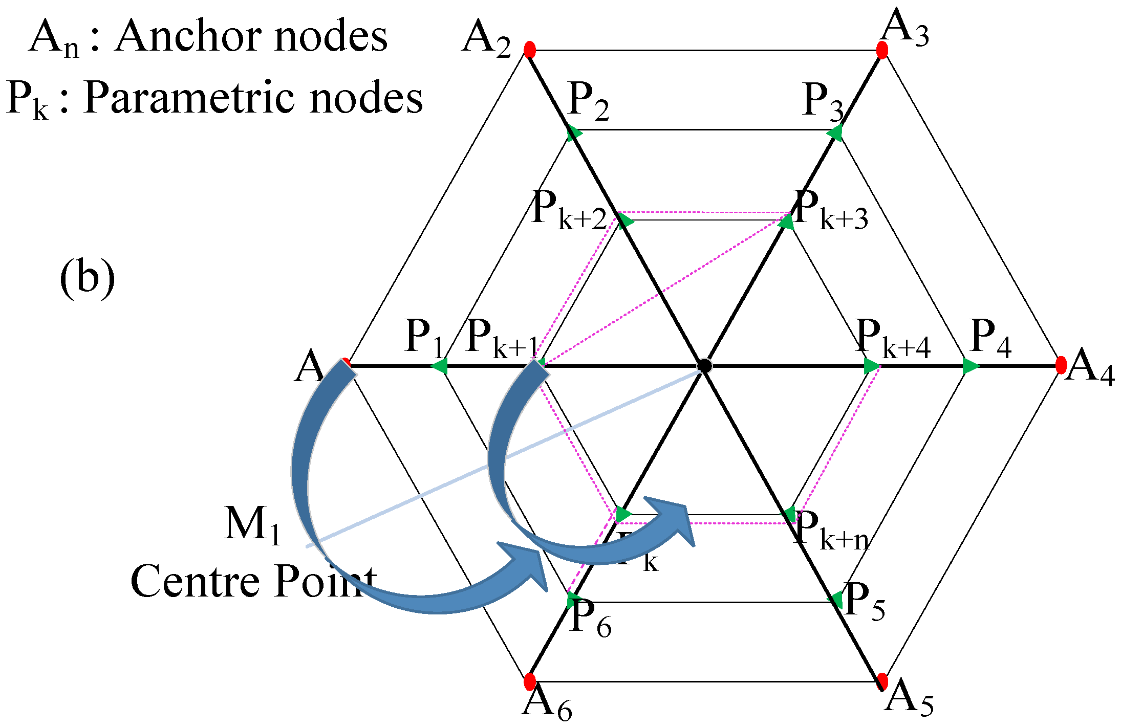
The basic principal of PLD localization algorithm is to find the actual 3D localization volume and compute the actual position of node. At each step part of triangle are subdivided with an addition of extraordinary nodes in its control ring matrix. For triangle formulation three nodes are required for centroid. We select the nearest node as a reference point and produce new parametric points with the help of those extraordinary nodes. This work involves the development of novel solution for ZigBee-based localization and utilizes the knowledge of fixed node positions to calibrate nodes with unknown positions. This will allow the positioning systems to adapt themselves in a changing environment, thereby increasing accuracy and reliability. New parametric points are produced with the help of those reference points. Inner node distribution of parametric node using Loop division is found in triangulation form as shown in Figure 2.
The key notations used in the proposed PLD scheme are summarized in Table 1.

3.2. System Model and Assumptions

Consider a non-overlapping network K = { k 1 , k 2 , , k n } with volume V = { v 1 , v 2 , , v n } . Assuming that a network with N sensor nodes and A anchor nodes randomly deployed in a field such as:
N = { N i ( x i , y i , z i ) , A i ( x i , y i , z i ) , D N N , D N A }
similarly each anchor node form a set of parameters:
A = { N i ( x i , y i , z i ) , A i ( x i , y i , z i ) , D A N , D A A }
where x i , y i , z i are the i th node coordinates and i = 1 , 2 , 3 , , n . The physical distance between two sensor nodes n i and n j is d ij = ( n i n j ) 2 . The PLD objective gives an insight into the actual estimation error that can be introduced with its dependence noise. The distance estimation will be carried out based on the statistical RSSI measurement model
R S S I i , j = P T P L i , j + i , j
where P T (dBm) is a transmission power of device used in measurement phase. The path-loss from the signal transmission is derived as:
P L i , j = l 0 10 n log 10 ( d i , j d 0 )
l 0 (dB) is the reference pathloss value at d 0 = 1 (m). n is the path loss exponent value for showing the environment characteristic. d i , j is the distance between node i and j in 3D modeling system.
d i , j = ( x i x j ) 2 + ( y i y j ) 2 + ( z i z j ) 2
Noise for line of sight (LOS) and non-line of sight (NLOS) scenarios is modeled as:
i , j = v i , j L O S ; v i , j + b N L O S N L O S ;
ρ i , j L O S = 1 2 π σ i , j 2 exp ( i , j 2 2 σ i , j 2 )
ρ i , j N L O S = 1 2 π σ i , j 2 exp ( ( i , j μ b ) 2 2 σ i , j 2 )
ρ i , j N L O S = 1 β τ i , j n m a x σ i , j τ i , j n m i n σ i , j
where v i , j is the measurement noise, v i , j ( 0 , σ i , j 2 ) , followed by various distributions such as Gaussian distribution, uniform distribution, and exponential distribution. β is a NLOS fractional noise calculated by β = n m a x n m i n with CDF τ . The value of b N L O S follows the Gaussian distribution as v i , j ( μ b , σ b 2 ) , so the PDF for NLOS will be modified as Equation (8). The standard normal distribution is further converted to τ as modeled in Equation (9). While, for exponential distribution function b N L O S ( λ ) , the PDF of i , j is given by:
ρ i , j N L O S = λ 2 exp [ λ i , j λ 2 σ i , j 2 2 ϕ λ 2 σ i , j 2 2 σ i , j ]
where λ is the positive constant and ϕ is the complementary error function. According to various distribution of NLOS noise condition, the suitable modeling scheme for indoor environment assumes uniform distribution due to the high variation in RSSI data and its multipath fading transmission modeled in Appendix A.

3.3. PLD Algorithm Design

PLD algorithm is described in several steps.
  • Deployed enough anchor nodes at the boundary of the PLD network. Assume an anchor node A i is reference anchor who initiate the process and select another two nodes to form a triangle. To gain a proper operation the PLD network size should be greater than 3.
  • Then the mid point is calculated with in the control ring matrix with the help of reference anchor node.
  • The parametric points are generated based on threshold value that jump the control over the parametric point in inner control vertex computed by (14).
  • RSSI is checked at each parametric point from anchor nodes computed by (11).
    R S S I = P T P L + F D
    where P T , P L , and F D are transmission power, path loss factor and fading respectively.
  • Center point increment (upward and downward) is obtained by addition and subtraction of step size over the network boundary. Furthermore, if threshold value is greater then the RSSI value the nodes is assumed as a pre-localized node as located inside the current ring matrix and stored the pre-localized nodes values in a storage network.
  • The product of each coordinates maximum and minum value in a control matrix is assumed as a localization volume that is computed by V = ( x m a x x m i n ) ( y m a x y m i n ) ( z m a x z m i n ) [3]. Localization points then can be computed by measuring the volume of pre-localizaed node boundary in Cartesian coordinate form.
  • Finally we can compute the localization error.

3.4. PLD Algorithm with Noise Modeling

Consider a system with a set of anchor nodes are A = { A 1 , A 2 , A 3 , A m } , where m 4 . An initiator, known as reference anchor, select two other nodes to form a parametric triangle. Computation of the midpoint of a link between two anchor nodes with the maximum distance. Let A 1 be a reference node, the total distance between the k t h selected nodes is determined from combination of ideal distance, mixed with noise:
D i k = k = 2 m D A k + A , k
where A , k is the Gaussian noise based on path-loss exponent value. The Gaussian noise is calculated by random number generator for initial simulation.
A , k = L O S T + r a n d ( m , 1 ) ; L O S = r a n d i ( [ n m i n n m a x ] , 1 , m ) N L O S T + r a n d ( m , 1 ) ; N L O S = r a n d i ( [ n m i n n m a x ] , 1 , m )
The pathloss exponent value varies according to propagation condition. The typical values are 1 2 and 2 5 for LOS and NLOS scenarios respectively. The selection of another anchor node for midpoint calculation in a PLD network can be determined through the average formula [3]. Midpoints give the advantage of taking close location as extraordinary nodes and producing the new parametric points with the help of those extraordinary nodes. Each anchor node will act as a control vertex in the first iteration, then transfer the control to the next parametric point that forms a ring matrix by Equation (14). The next step is to check RSSI from anchor nodes at each parametric point that is stored in a matrix.
P i k = 3 8 ( M 1 + A k ) + 1 8 ( A k 1 + A k + 1 )
f ( P R S S I ) = P r e l o c c o r d ( P R S S I ) t h r e s h o l d o t h e r w i s e
where P i k is a parametric point calculation. If the sum of RSSI values are smaller than the threshold value, it is chosen as a pre-localized node ( A i k ) and the iteration stops at this point. Due to noise the RSSI values will fluctuate. To minimize the adverse effect of noise, we can use weighting concept as intelligent and naive noise model as explained in Appendix B.

3.5. EKF Algorithms for PLD

The nonlinear nature of RSSI values in a noisy localization system motivates us to apply extended Kalman filter (EKF). Due to multiplicative noise effect in the localization system, EKF can help to refine the PLD process. There are three types of EKF that are widely used in positioning system, namely P-model (position), PV-model (position, velocity) and PVA (position, velocity, acceleration) [27]. According to the PLD scheme that only used RSSI, distance and reference coordinate for determining the unknown node position, P-model EKF is chosen. To apply the P-model EKF, three phase, initialization, prediction and update are described as follows.
Initialization State: This step is basically modeled the equation and using EKF algorithm as follows:
x k = f ( x k + 1 ) + W k 1 x k = f ( x k + 1 · t k ) + W k 1 · t k 1 z k = h ( x k ) + v k z k = h ( x k ) · t k + v k · t k
where W k 1 represents the noise factor of EKF having normal distribution with zero average value and its co-variance matrix Q k and R k , i.e., W k 1 ( 0 , Q k ) and W k 1 ( 0 , R k ) . x k and x k 1 are the state vectors at time instants t k and t k 1 . While f is the non-linear function used to predict data information based on historical data, and the h function describes the correlation state among x k and z k .
Prediction State: This step involves, predicted variable that has been declared in initialization state. Priori state x ^ k k 1 processed the previous information data from posteriori state:
x ^ k k 1 = F · x ^ k 1 k 1 + B k · u k P k k 1 = F · P k 1 k 1 F T + Q
where u k denotes the input system, F is the transition matrix and B k is the input matrix. The variable of P k k 1 and P k 1 k 1 are the information state gain from co-variance data matrix Q.
Update State: The output from this state is the estimation result. There is an inovation vector Y ^ k from Equation (16) which is modified as follow:
Y ^ k = z k h ( x ^ k ) S k = H k · P k k 1 · H k T + R K x ^ k k = x ^ k k 1 · K k · Y ^ k K k = P k k 1 · H k T · S k 1 P k = ( l d K k · H k ) · P k k 1
where H k is the is the Jacobian matrix based on expected measurement result value from h ( x ^ k ) . The posteriori state which is the estimation result from EKF algorithm calculated from above Equation (18). In our proposed PLD scheme with noise suppression, the distance values with noise will be used for localization and then EKF is used to refine the PLD estimation results. There are two estimation process at this system: (1) one is the PLD algorithm based on volume pre-localized node boundary calculation (2) the other is using EKF to reduce the noise from PLD algorithm. The combination of PLD algorithm and EKF algorithm will be processed by three steps involve initialization state, predict state and update state.
x k = P L D R S S I , [ f ( x i y i z i ) ]
For the PLD algorithm [3], there are five or six reference distance values from unknown nodes to the anchor nodes in case of 6 anchor nodes in a working boundary z k = [ d 1 d 2 d n ] d n . The output coordinates from PLD algorithm with noise modeling will be used for co-variance matrix of EKF algorithm which, is derived as follows:
P 0 = σ 2 x P L D , 0 0 0 0 0 σ 2 y P L D , 0 0 0 0 0 σ 2 z P L D , 0 0 0 0 0 0 0 0 0 0 0 0
Each variable, including initialization state and co-variance matrix that has been declared, will be predicted to the next state using:
x k = P L D [ x i y j z k ] F f = 1 0 0 0 0 0 1 0 0 0 0 0 1 0 0 0 0 0 0 0 0 0 0 0 0
P k = F P 0 F T + Q Q = P 0
where P k is the co-variance information and Q is the co-variance matrix. The predicted state output from Equations (21) and (22) is the updated data which should be multiplied with Kalman filtering gain K k then we have:
K k = P k · H k T · S k 1
H k is the observation data matrix in update state, represented by Jacobian matrix. This matrix is obtained from comparison data between coordinate output x P L D , y P L D , z P L D , and estimated distance of PLD algorithm with noise modeling ( P L D ) . Finally,
H k σ = x 1 x 1 ^ d 1 y 1 y 1 ^ d 1 z 1 z 1 ^ d 1 x 2 x 2 ^ d 2 y 2 y 2 ^ d 2 z 2 z 2 ^ d 2 x n x n ^ d n y n y n ^ d n z n z n ^ d n
d n = ( x i x i ^ ) 2 + ( y j y j ^ ) 2 + ( z k z k ^ ) 2
Another covariance matrix, S k , which is calculated by combination of covariance matrix P k with noise co-variance of estimated distance R k from original PLD estimation, can be derived as:
S k = H k · P k · H k T + R k R k = d i a g ( σ 2 d 1 σ 2 σ 2 d n ) P 0 = ( P k K k H k ) P k
The posterior state as the estimation result of EKF algorithm ( X E K F , Y E K F ) is represented as:
Y k = z k h k h k = [ d 1 d 2 d n ] X k + 1 = X k + K k · Y k
The flowchart of the proposed noisy PLD scheme with EKF is shown in Figure 3.

4. Simulation and Results

This section, provides a comprehensive evaluation of the PLD algorithm through simulation experiments on Matlab. Anchor nodes are randomly deployed within 100 m × 100 m × 100 m 3D area. The number of anchor nodes in each simulation is set to 5 and, at each step, the location of anchor node is changed randomly. The simulation was run for 1000 iterations which make the deployment area to cover 5000 anchor nodes. The number of localization points on PLD is directly proportional to the volume of Pre-localized nodes. As each node has localization error distance so we are interested in calculating mean error distance with constant sensing unit volume. Mean localization error (MLE) is calculated by the fraction of the number of nodes and sum of error distance. Table 2 shows the random deployment of anchor nodes that produces four localized point as the target node. Experiment shows the sum of localization error is 3.57 m and Mean localization error is 0.89 m as shown in Figure 4 [3].
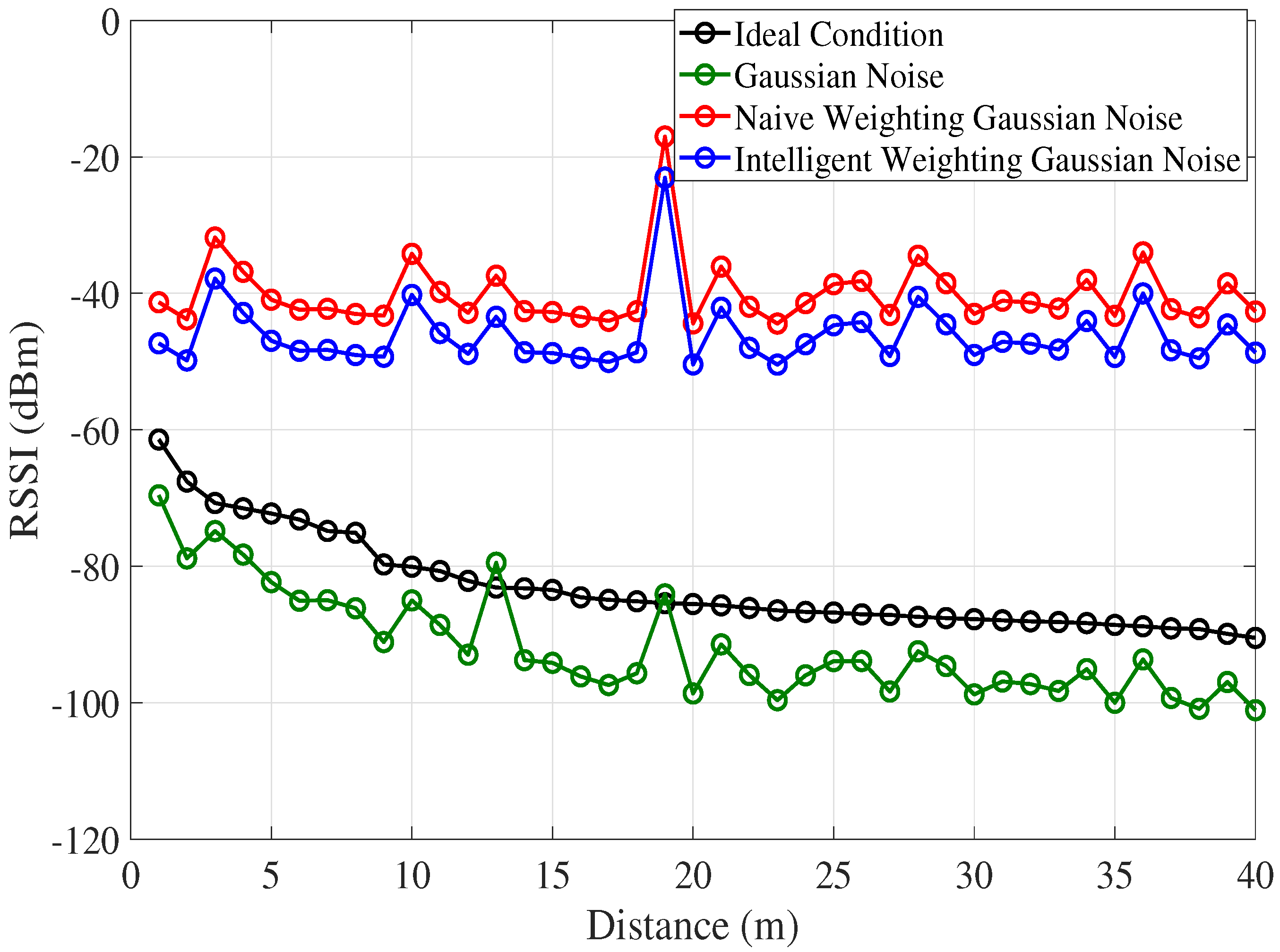
In indoor environment, RSSI values fluctuate and even get weaker in longer distance as shown in Figure 5. The RSSI data with Gaussian noise can describe in real condition then, for reducing the large variation in RSSI, we add another modelling noise such as naive and intelligent noise which have small fluctuation in longer distance.
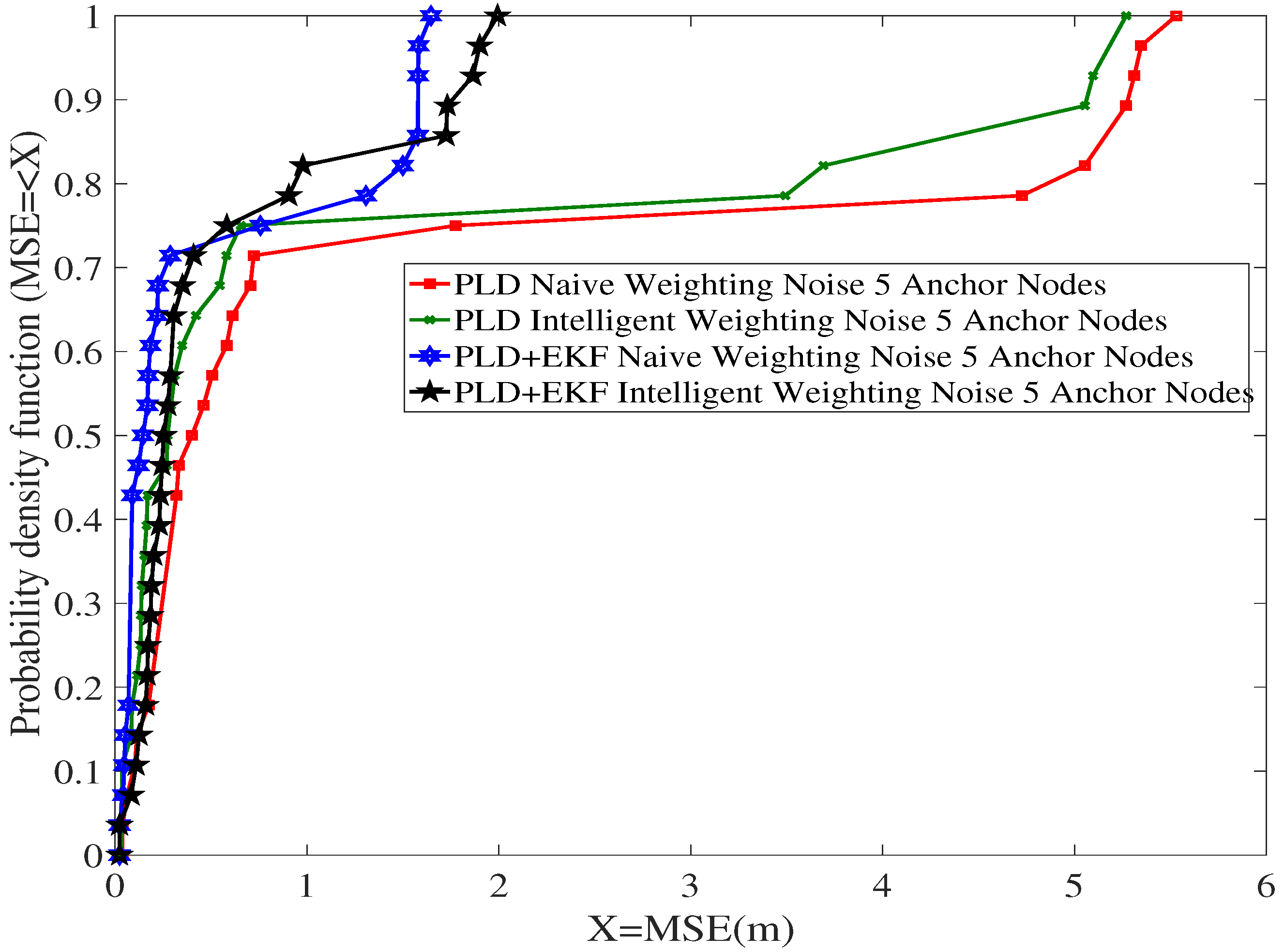
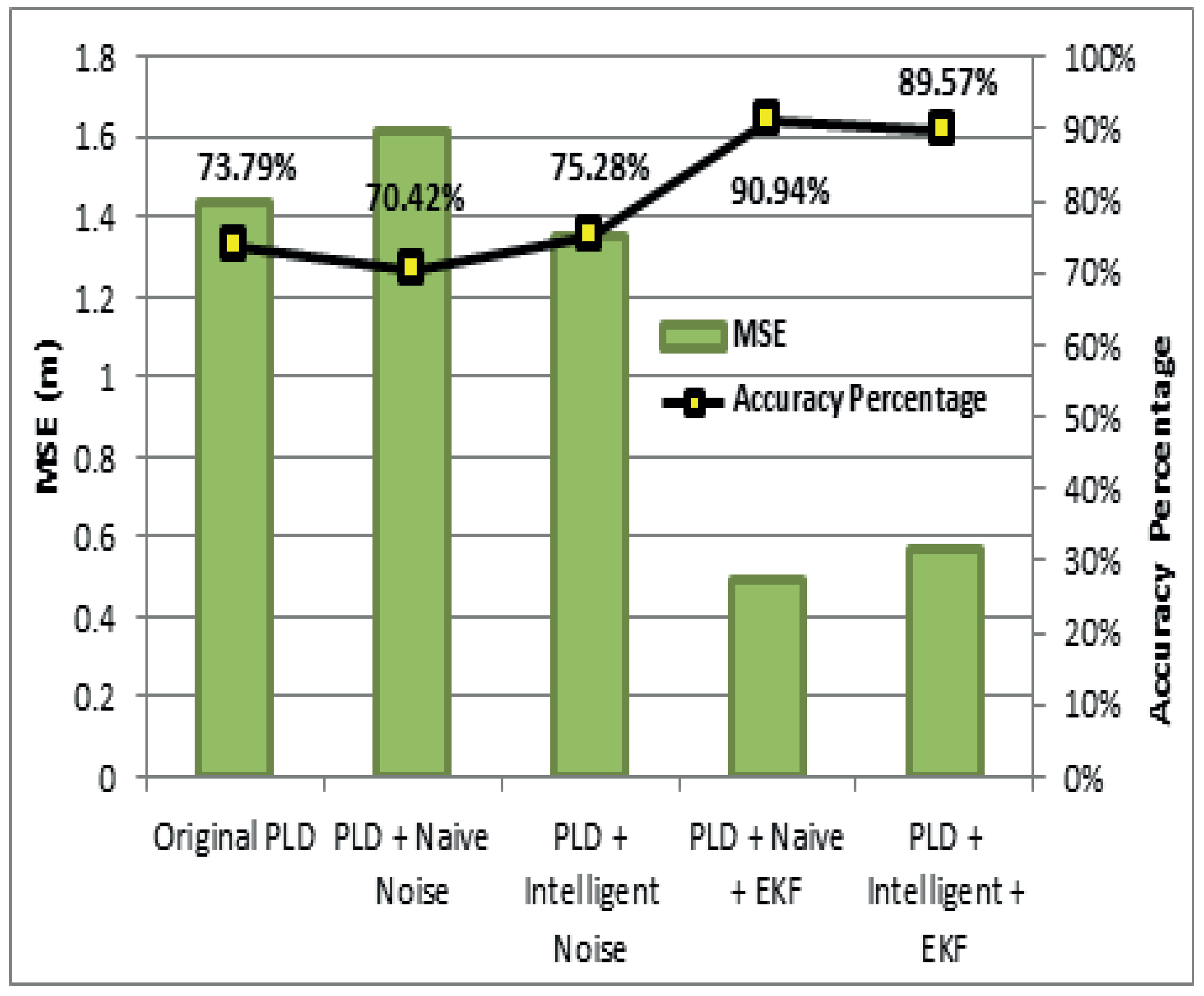
The localization accuracy of this system can be analyzed in overall data using cumulative distribution function (CDF) as shows in Figure 6. This graph is used to know the smallest MSE value based on cumulative probability for each method. There are three factors that can affect the localization accuracy. Those are the number of anchor nodes, noise type and localization algorithm. Based on the type of algorithm at five anchor nodes, The best performance is achieved by PLD + EKF algorithm as shown in Figure 3 with 5 anchor nodes, the combination of PLD and EKF algorithm with naive noise has an error distance between 0.042 m to 1.64 m, while adding intelligent noise to the PLD + EKF algorithm leads to an error distance range between 0.023 m to 1.99 m. It is very different with the conventional PLD algorithm [6] without refinement process by EKF algorithm. The overall average estimation error is achieved up to 1.8 m in presence of naive and intelligent noise. The result show using the combined PLD and EKF algorithm with intelligent and naive noise have high accuracy up to the 89.57% as shown in Figure 7.

5. Conclusions

In this paper, we proposed a noise-reduced PLD algorithm with EKF. PLD is capable of finding its own localized node within its working boundary. Reference points are considered to produce mid-points, parametric points and step size, which helps the iterative control to be transferred to inner parametric points. This enables PLD to work in different networks, within the working boundary. At each reference point, sum of RSSI value is computed for pre-localized nodes, compared to a threshold value, and stored in a storage matrix. Furthermore, the localization volume is obtained with maximum and minimum coordinates, stored in a storage matrix. Compared with the refined coordinates, PLD provide an overall efficiency of 87.57% even in noisy condition. The effectiveness of PLD-EKF were verified by extensive simulation in different distances and number of nodes.

Author Contributions

T.A. and X.J.L. conceived and designed the idea and perform simulations. T.A. derived the idea, where as X.J.L. contributed to the analysis and modeling part of the work. B.-C.S. provided comments and helped to evaluate and edit the manuscript.

Funding

This work was funded by the Vice Chancellor Doctoral Scholarship at Auckland University of Technology, New Zealand.

Conflicts of Interest

The authors declare no conflict of interest.

Abbreviations

The following abbreviations are used in this manuscript:
PLDParametric loop division
GPSGlobal positioning system
ToATime of Arrival
TDoATime difference of Arrival
AoAAngle of Arrival
RSSIReceived signal strength Indicator
APSAd-hoc positioning system
MDSMultidimensional scaling
APITApproximate Point in triangulation
LOSline of sight
NLOSNon-line of sight
EKFExtended Kalman filtering

Appendix A

The noise includes additive noise to the distances:
d i , j = ( x i x j ) 2 + ( y i y j ) 2 + ( z i z j ) 2 + i , j
while the noise model mostly used is multiplicative as follows:
d i , j = ( x i x j ) 2 + ( y i y j ) 2 + ( z i z j ) 2 + 1 + i , j
= i , j L O S 0 , ( x i x j ) 2 + ( y i y j ) 2 + ( z i z j ) 2 2 σ i , j 2
= i , j N L O S ( x i x j ) 2 + ( y i y j ) 2 + ( z i z j ) 2 2 σ i , j 2 m i n , ( x i x j ) 2 + ( y i y j ) 2 + ( z i z j ) 2 2 σ i , j 2 m a x
Let’s assume the d l i , j = ( x i x j ) 2 + ( y i y j ) 2 + ( z i z j ) 2 as the ideal distance without noise influence. Practical RSSI data have high noise variations and it is suitable for adding the weight that can develop approximations of log-likehood function in the sophisticated noise model. The weights can be written as γ = 1 σ i , j 2 d i , j 2 , so this noise modeling system is known as intelligent noise as:
= i , j ϵ 1 , 2 , 3 N 1 d l i , j 2 σ i , j 2 d l i , j d i , j
In case of Intelligent weighting the noise is scaled based on the distance that is not reliable for long distances due to less weight. In that case naive Bayesian noise model is a best solution expressed as:
= i , j ϵ 1 , 2 , 3 N 1 d l i , j 2 σ i , j 2 log d l i , j log d i , j

Appendix B

Intelligent noise:
D i n t . n o i s e = k = 1 m D i k + 1 D k 2 + v a r ( D k 2 ) x ( l D k D k ) 2
Naive noise:
D n a i v e . n o i s e = k = 1 m D i k + 1 D k 2 + v a r ( D k 2 ) x ( log l D k log D k ) 2
Then the combination of intelligent and noise model that forms the multiplicative noise that can be calculated as:
D m u l . n o i s e = k = 1 m [ 1 D k 2 + v a r ( D k 2 ) x ( l D k D k ) 2 + 1 D k 2 + v a r ( D k 2 ) x ( log l D k log D k ) 2 ]

References

  1. Ahmad, T.; Li, X.J.; Seet, B.C. 3D localization based on parametric loop division and subdivision surfaces for wireless sensor networks. In Proceedings of the 2016 25th Wireless and Optical Communication Conference (WOCC), Chengdu, China, 21–23 May 2016; pp. 1–6. [Google Scholar]
  2. Ahmad, T.; Li, X.J.; Seet, B.C. A self-calibrated centroid localization algorithm for indoor ZigBee WSNs. In Proceedings of the 2016 8th IEEE International Conference on Communication Software and Networks (ICCSN), Beijing, China, 4–6 June 2016; pp. 455–461. [Google Scholar]
  3. Ahmad, T.; Li, X.J.; Seet, B.C. Parametric loop division for 3d localization in wireless sensor networks. Sensors 2017, 17, 1697. [Google Scholar] [CrossRef] [PubMed]
  4. Karalar, T.C.; Rabaey, J. An RF ToF Based Ranging Implementation for Sensor Networks. In Proceedings of the 2006 IEEE International Conference on Communications (ICC), Istanbul, Turkey, 11–15 June 2006; pp. 3347–3352. [Google Scholar]
  5. Cheng, X.; Thaeler, A.; Xue, G.; Chen, D. A Time-Based Positioning Scheme for Outdoor Wireless Sensor Networks. In Proceedings of the 2004 Twenty-Third AnnualJoint Conference of the IEEE Computer and Communications Societies (INFOCOM), Hong Kong, China, 7–11 March 2004; pp. 2685–2696. [Google Scholar]
  6. Sayed, A.H.; Tarighat, A.; Khajehnouri, N. Network-based wireless location: Challenges faced in developing techniques for accurate wireless location information. IEEE Signal Proc. Mag. 2005, 22, 24–40. [Google Scholar] [CrossRef]
  7. Jiang, J.-A.; Zheng, X.-Y.; Chen, Y.-F.; Wang, C.-H.; Chen, P.-T.; Chuang, C.-L.; Chen, C.-P. A distributed RSS-based localization using a dynamic circle expanding mechanism. IEEE Sens. J. 2013, 13, 3754–3766. [Google Scholar] [CrossRef]
  8. Zhong, Z.; He, T. Achieving range-free localization beyond connectivity. In Proceedings of the 7th ACM Conference on Embedded Networked Sensor Systems, Berkeley, CA, USA, 4–6 November 2009; pp. 281–294. [Google Scholar]
  9. Yang, X.; Kong, Q.; Xie, X. One-dimensional localization algorithm based on signal strength ratio. Int. J. Distrib. Sens. Netw. 2009, 5, 79. [Google Scholar] [CrossRef]
  10. Fang, Z.; Zhao, Z.; Cui, X.; Geng, D.; Du, L.; Pang, C. Localization in wireless sensor networks with known coordinate database. EURASIP J. Wirel. Commun. Netw. 2010, 2010, 901283. [Google Scholar] [CrossRef]
  11. Zhu, X.; Wu, X.; Chen, G. Relative localization for wireless sensor networks with linear topology. Comput. Commun. 2013, 36, 1581–1591. [Google Scholar] [CrossRef]
  12. Karalar, T.C.; Yamashita, S.; Sheets, M.; Rabaey, J. A Low Power Localization Architecture and System for Wireless Sensor Networks. In Proceedings of the 2004 IEEE Workshop on Signal Processing Systems (SIPS), Austin, New Zealand, 13–15 October 2004; pp. 89–94. [Google Scholar]
  13. Hightower, J.; Want, R.; Borriello, G. Spoton: An Indoor 3D Location Sensing Technology Based on RF Signal Strength; UW CSE 00-02-02; University of Washington, Department of Computer Science and Engineering: Seattle, WA, USA, 2000. [Google Scholar]
  14. Niculescu, D.; Nath, B. DV based positioning in ad hoc networks. Telecommun. Syst. 2003, 22, 267–280. [Google Scholar] [CrossRef]
  15. Ahmad, T.; Li, X.J.; Seet, B.-C. Fuzzy-Logic Based Localization for Mobile Sensor Networks. In Proceedings of the 2019 2nd International Conference on Communication, Computing and Digital systems (C-CODE), Islamabad, Pakistan, 6–7 March 2019; pp. 43–47. [Google Scholar]
  16. Luo, Z.; Cui, X.; Zhang, W.; Lu, J. Calculation of the 3-D ionized field under HVDC transmission lines. IEEE Trans. Magn. 2011, 47, 1406–1409. [Google Scholar] [CrossRef]
  17. Zàruba, G.V.; Huber, M.; Kamangar, F.; Chlamtac, I. Indoor location tracking using RSSI readings from a single Wi-Fi access point. Wirel. Netw. 2007, 13, 221–235. [Google Scholar] [CrossRef]
  18. Wu, C.L.; Fu, L.C.; Lian, F.L. WLAN location determination in e-home via support vector classification. In Proceedings of the 2004 IEEE International Conference on Networking, Sensing and Control, Taipei, Taiwan, 21–23 March 2004; pp. 1026–1031. [Google Scholar]
  19. Chen, Y.; Yang, Q.; Yin, J.; Chai, X. Power-efficient access-point selection for indoor location estimation. IEEE Trans. Knowl. Data Eng. 2006, 18, 877–888. [Google Scholar] [CrossRef] [Green Version]
  20. Youssef, M.; Agrawala, A. The Horus location determination system. Wirel. Netw. 2008, 14, 357–374. [Google Scholar] [CrossRef]
  21. Au, A.W.S.; Feng, C.; Valaee, S.; Reyes, S.; Sorour, S.; Markowitz, S.N.; Gold, D.; Gordon, K.; Eizenman, M. Indoor tracking and navigation using received signal strength and compressive sensing on a mobile device. IEEE Trans. Mob. Comput. 2013, 12, 2050–2062. [Google Scholar] [CrossRef]
  22. Cheng, F.-H.F.; Fan, F.-T.; Lai, S.-H.; Huang, C.-L.; Wang, J.-X.; Yong, J.-H. Loop subdivision surface based progressive interpolation. J. Comput. Sci. Technol. 2009, 24, 39–46. [Google Scholar] [CrossRef]
  23. ZigBee Alliance, ZigBee Specification. Version 1.0 ZigBee Document 053474r06, December 14th. 2004. Available online: https://www.zigbee.org/zigbee-compliant-platforms/ (accessed on 29 April 2019).
  24. He, T.; Huang, C.; Blum, B.M.; Stankovic, J.A.; Abdelzaher, T. Range-free localization schemes for large scale sensor networks. In Proceedings of the 9th Annual International Conference on Mobile Computing and Networking, San Diego, CA, USA, 14–19 September 2003; pp. 81–95. [Google Scholar]
  25. Ahmad, T.; Li, X.J.; Seet, B.C. 3D Localization Using Social Network Analysis for Wireless Sensor Networks. In Proceedings of the 2018 IEEE 3rd International Conference on Communication and Information Systems (ICCIS), Singapore, 28–30 December 2018; pp. 88–92. [Google Scholar]
  26. Ma, Z.; Liu, Y.; Shen, B. Distributed locating algorithm for wireless sensor networks-MDS-MAP. J. Commun. 2008, 29, 57–62. [Google Scholar]
  27. Zhu, Y.; Shareef, A. Comparisons of three kalman filter tracking algorithms in sensor network. In Proceedings of the 2006 International Workshop on Networking, Architecture, and Storages (IWNAS’06), Shenyang, China, 1–3 August 2006. [Google Scholar]
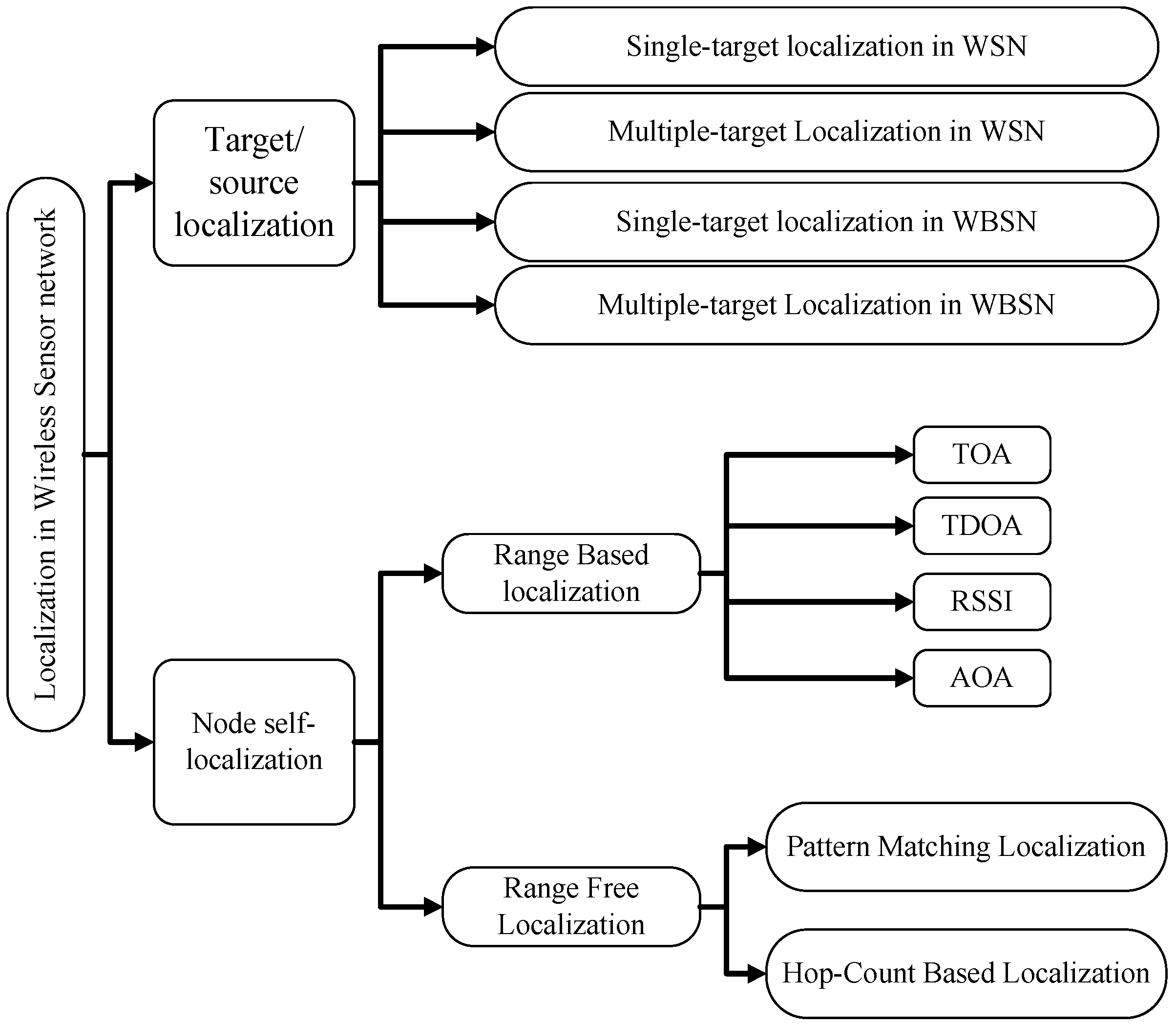
Figure 1. Classification of localization algorithms.
Jsan 08 00024 g001
Figure 2. Parametric point calculation in PLD algorithm.
Jsan 08 00024 g002
Figure 3. Extended Kalman filtering implemented on PLD coordinates.
Jsan 08 00024 g003
Figure 4. Mean square error of PLD with different localization volumes.
Jsan 08 00024 g004
Figure 5. Distance vs. RSSI.
Jsan 08 00024 g005
Figure 6. Mean square error vs. distance.
Jsan 08 00024 g006
Figure 7. PLD performance in presence of naive, intelligent noise.
Jsan 08 00024 g007
Table 1. List of key notations.
NotationExplanation
M i Mid points of each PLD network
A i i th anchor node
P i i th parametric points produced after each iteration
N i Volume of i th parametric looped network
k i Non overlapped PLD networks
D N N Distance matrix from a sensor node N i to all other sensors in a network
D A N Distance matrix from a anchor node A i to all other sensors in a network
φ Targetted node in each k i network
η Number of generated anchor nodes in k i network
Δ Step size in PLD network
α Parametric function of PLD network
γ Representation of change in center point
ξ Working boundary
x ^ , y ^ , z ^ Cartesian coordinates of estimated node position.
v i , j Measurement noise
β NLOS fractional noise
Noise to PLD coordinates
λ positive constant
ϕ complementary error function
P i k Parametric points
hcorrelation state in EKF initialization
x ^ k k 1 priori state
Qco-variance matrix
Table 2. Localization error of four nodes in each PLD network.
x ^ ŷxyzError in (m)
14.477.6614.1115.908.2015.271.91
15.549.9314.9015.549.9314.901.53
15.7310.6515.2515.7910.6315.270.05
16.9311.8516.4516.9411.8516.150.08