Article

On-Line RSSI-Range Model Learning for Target Localization and Tracking

by
José Ramiro Martínez-de Dios
1,*,
Anibal Ollero
1,
Francisco José Fernández
2 and
Carolina Regoli
3
1
Robotics Vision and Control Group, Universidad de Sevilla, Escuela Superior de Ingenieros, c/Camino de los Descubrimientos s/n, 41092 Seville, Spain
2
Universidad de Sevilla, Escuela Superior de Ingenieros, c/Camino de los Descubrimientos s/n, 41092 Seville, Spain
3
Central University of Venezuela, Ciudad Universitaria s/n, Caracas 1050, Venezuela
*
Author to whom correspondence should be addressed.
J. Sens. Actuator Netw. 2017, 6(3), 15; https://doi.org/10.3390/jsan6030015
Submission received: 8 May 2017 / Revised: 30 July 2017 / Accepted: 5 August 2017 / Published: 10 August 2017
(This article belongs to the Special Issue QoS in Wireless Sensor/Actuator Networks and Systems)

Abstract

:
The interactions of Received Signal Strength Indicator (RSSI) with the environment are very difficult to be modeled, inducing significant errors in RSSI-range models and highly disturbing target localization and tracking methods. Some techniques adopt a training-based approach in which they off-line learn the RSSI-range characteristics of the environment in a prior training phase. However, the training phase is a time-consuming process and must be repeated in case of changes in the environment, constraining flexibility and adaptability. This paper presents schemes in which each anchor node on-line learns its RSSI-range models adapted to the particularities of its environment and then uses its trained model for target localization and tracking. Two methods are presented. The first uses the information of the location of anchor nodes to dynamically adapt the RSSI-range model. In the second one, each anchor node uses estimates of the target location—anchor nodes are assumed equipped with cameras—to on-line adapt its RSSI-range model. The paper presents both methods, describes their operation integrated in localization and tracking schemes and experimentally evaluates their performance in the UBILOC testbed.

1. Introduction

The Received Signal Strength Indicator (RSSI) is a main metric to estimate Quality of Service (QoS) of wireless links [1]. RSSI can be measured by the radio modules of most Commercial Off The Shelf (COTS) Wireless Sensor Network nodes with negligible cost in energy, delay and computational effort. The strength of the radio signals attenuates with distance as they propagate. Hence, a receiver can measure the RSSI of an incoming packet, estimate the distance and use it to find out the location of the emitter. Many RSSI-based localization methods have been researched and proposed over the years. One of the main drawbacks of using RSSI to estimate WSN link QoS in general—and also to estimate the distance between two WSN nodes—is that the strength of radio signals is highly affected by reflections and other interactions of the radio signal with the environment. These interactions are very difficult to be modeled and highly disturb the accuracy of RSSI-based localization techniques. In fact, many methods, e.g., range-free localization methods, compute location estimates without transforming RSSI into distance and hence, avoiding the inaccuracies of RSSI-range models.
Some techniques adopt a training-based approach in which they off-line learn the RSSI-range characteristics of the environment in a prior training phase and then, use the learned characteristics during the localization phase. In these methods the training phase is a long off-line time-consuming process. Besides, the training phase must be repeated if there have been changes in the environment.
This paper presents methods that address the learning of RSSI-range characteristics of the environment as an on-line process, i.e., training is performed during localization, enabling high adaptability to scenario changes. In this paper two methods are presented and compared. The first one uses the information of the location of the static nodes to dynamically adapt the RSSI-range model. The second one uses information gathered by nodes equipped with additional sensors—cameras—to continuously learn accurate RSSI-range models adapted to the local environment of the emitter and receiver nodes. The presented methods are efficient, scalable, operate in real-time and only require a few measurements to compute updated RSSI-range models. They are integrated in a target localization and tracking scheme that employs the trained RSSI-range models, significantly reducing target tracking errors. The paper presents both on-line RSSI-range model learning methods, describes their operation and experimentally evaluates their performance in the UBILOC Testbed.
This paper is structured as follows. Section 2 summarizes the related work. The problem formulation and general description of the presented methods are presented in Section 3. The two on-line RSSI-range model learning methods are described in Section 4 and Section 5. Section 6 presents some experiments and discusses on the presented methods and results. The conclusions are in Section 7.

2. Related Work

RSSI is the most widely researched and employed measurement in localization and tracking in WSN. A high number of RSSI-based localization systems have been developed. Range-based methods, such as multilateration [2] or least squares [3], among many others, use RSSI measurements to estimate the distance to anchor nodes. Reflections and other interactions with the environment make RSSI-range models very dependent on the specific setting, making them unpredictable. Most range-based methods adopt a general RSSI-range model—such as references [4,5]—that assume free-space radio propagation and consider these perturbations as noise. Range-free methods, such as ROC-RSSI [6] or APIT [7], use geometrical considerations for localization instead of RSSI-range models. Although more robust to perturbations in the radio channel, their localization errors are usually higher than those of range-based techniques.
Another approach is to learn RSSI-range characteristics from the environment. In general, RSSI training-based localization and tracking includes two phases: (i) the training phase, where the RSSI-range characteristics of the environment are captured using measurements gathered in the scenario and represented typically in maps and; (ii) the localization phase, where the location estimation is performed using the RSSI map and the current RSSI measurements. The training phase is an off-line process that needs to be repeated if there have been changes in the wireless propagation environment. RSSI training-based techniques can be broadly divided into deterministic and probabilistic methods.
Deterministic RSSI training-based localization techniques include references [8,9]. In the training phase the environment is subdivided into small cells and, RSSI measurements are gathered in these cells from several anchor nodes, which location is assumed known. In the localization phase the RSSI measurements from the target are gathered and the cell in the RSSI map that best fits with the current measurements is selected as the target location. Probabilistic RSSI training-based localization methods include references [10,11]. A probability distribution of the target location is defined over the area of the environment. The goal of the localization phase is to reach a single mode for this distribution, which is the most likely location of the target. In these methods a Bayesian belief network is established and trained with a preset number of discretized location possibilities (cells).
The aforementioned RSSI training-based localization methods rely on long training phases where a RSSI map of the entire target area is built with some spatial precision. This precision will have a great impact on the accuracy of the localization estimate. Such data collection/measurement for RSSI map building requires significant labor. Besides, the map must be recomputed whenever the wireless propagation properties may change. Thus, these methods cannot be applied in schemes that require quick deployment or in dynamic environments with frequent changes.
Modeling radio propagation characteristics with RSSI maps poses memory footprint issues when implementing these methods in COTS nodes. Some methods aim at building RSSI-range models trained for an specific environment. In reference [12] the authors evaluate ray-tracing techniques that are used to obtain indoor propagation models. In reference [13] a statistical approach is employed to build a wireless map based on statistical properties of the area. An even simpler and more practical approach is adopted in references [14,15]. In these methods RSSI-range models are computed using regressions but model fitting is designed as an off-line process, lacking flexibility and adaptability to environment changes.

3. On-Line RSSI-Range Training Problem Formulation

The objective of the presented method is to on-line obtain RSSI-range models adapted to the specific scenarios and environments. The local environment around two nodes critically impacts on the RSSI measurements between them. In fact, if we take RSSI measurements between two nodes without changing their local environments, we can notice that all the RSSI values are very similar. As an illustration Figure 1 shows 40,000 different RSSI measurements between one node and three other anchor nodes taken during 16 h in the UBILOC Testbed. Despite the high number of measurements, the difference between them was lower than 3 dBm and their standard deviation was lower than 1.4 dBm, which evidences the low level of noise in RSSI measurements when the environment surrounding the emitter and the receiver is static. This experiment was repeated in several occasions at different days and hours obtaining similar results. Thus, we can conclude that the main cause in the variability of RSSI measurements is not the random measurement noise itself, but changes in the environment surrounding the emitter and the receiver. Below a justification based on radio propagation is summarized.
Most localization methods use RSSI-range models that assume free-space propagation [4,5], and adopt expressions similar to the following, see Appendix A:
R S S I ( D ) = a log D + b ,
where R S S I ( D ) is the RSSI measured by a node from the packets it receives from the emitter node located at distance D from the receiver. a and b are the model parameters. This model assumes that the receiver sees only the direct radio signal transmitted by the emitter and, in this case, the RSSI measurement noise is statistically independent, as in the case of many other measurement processes. It should be noticed that the objective of model in (1) is to numerically relate RSSI and range. It can be easily derived from a general free-space radio propagation model.
However, the above model is ideal. In real cases the presence of reflectors in the environment creates multiple paths that a transmitted signal can traverse. As a result, the receiver sees the superposition of multiple copies of the transmitted signal, each of them traversing a different path. Each signal copy will experience different attenuation, delay and phase shift while traveling from the emitter to the receiver. The signal received is the composition of the direct signal and the contribution of these multiple copies. Hence, the signal strength of the resulting composition in a given environment is extraordinarily difficult to be modeled.
The most widely used approach in target localization and tracking methods is to adopt the model in (1)—i.e., propagation assuming no multi-path—and to consider the effects of multi-path propagation as noise. However, this noise is not originated by the randomness of the measurement process but by the influence of the particular environment surrounding the emitter and the receiver. This noise involves large errors in RSSI-range models and originates large localization and tracking errors. In recent years some few techniques for target localization under realistic correlated RSSI noise have been proposed [16] but they usually have bad scalability and involve computational loads that can be hardly implemented in COTS WSN nodes.
This work proposes methods that aim at capturing the overall effects of the full radio propagation using simple RSSI-range models that are trained continuously (on-line) during target tracking using updated RSSI measurements gathered by the anchor nodes deployed at the environment. In the presented methods each node dynamically trains its RSSI-range model using only the M most recent RSSI measurements. M = 7 was taken in the experiments. During this short interval, assuming moderate target motion, the environment—and hence the radio propagation conditions—can be considered static or almost static.
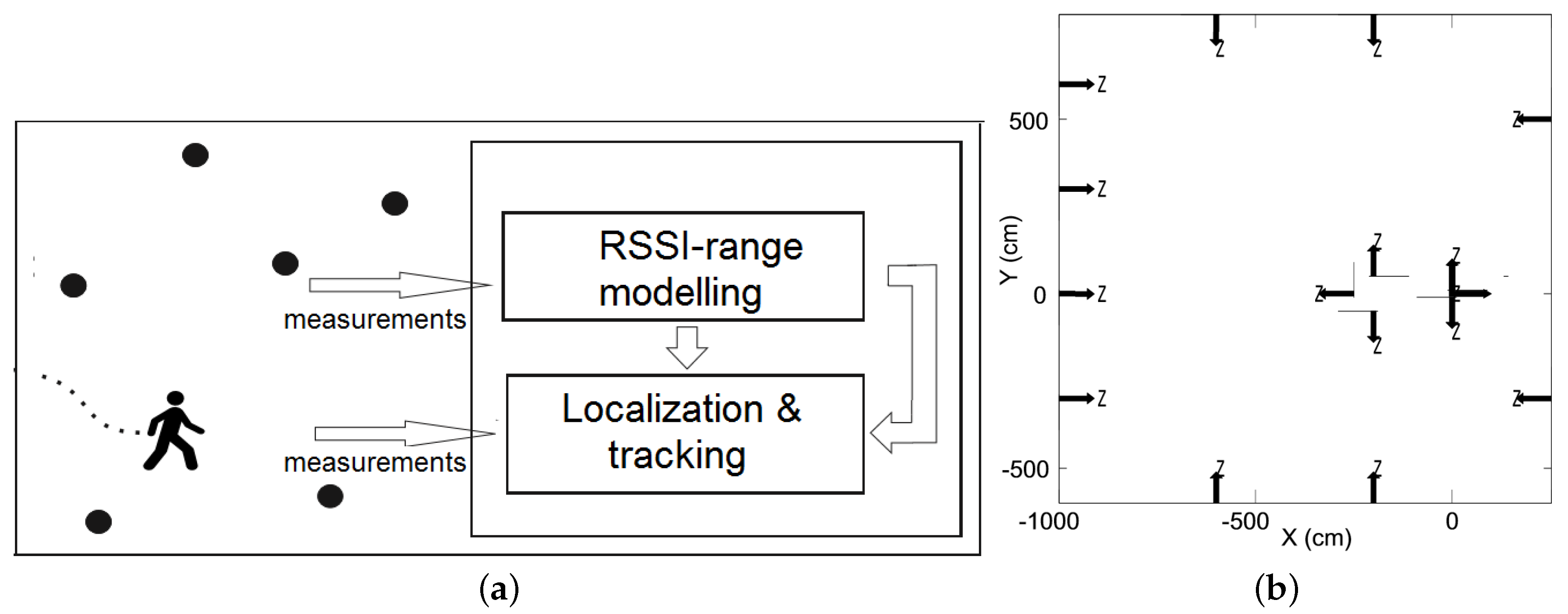
The paper presents two methods for on-line RSSI-range modeling and compares their performance in a target localization and tracking scheme, see Figure 2a. In the first method, described in Section 4, each anchor node uses inter-anchor RSSI measurements to dynamically train the RSSI-range model. In the second one, described in Section 5, each anchor node uses information gathered by external sensors—cameras—to continuously update and train RSSI-range models adapted to the environment conditions. In both cases, once computed, the trained RSSI-range model is used as the observation model in the target localization and tracking scheme in Figure 2a. Figure 2b shows an example of the geometrical setting of the experimentation scenarios. The optical axes of the cameras of the sensor nodes in the method described in Section 5 are shown.

4. On-Line Training Using Inter-Anchor RSSI Measurements

In this method, each anchor node dynamically computes its RSSI-range model using the RSSI measurements from the packets it interchanges with other anchor nodes. These measurements are used to on-line perform the RSSI-range model regression. The method is general and only assumes that each node knows its own location, which is reasonable and does not constrain its generality.

4.1. Inter-Anchor RSSI-Range Model Training

This method adopts the widely assumed model expressed in (1) in which RSSI-range is taken as a linear function between the RSSI and the logarithm of the distance D. Assuming a set of measurements of the type {( R S S I k , log D k )}, the model in (1) can be fitted by performing a simple linear least squares regression:
a = k R S S I k log D k R S S I ¯ k log D k k ( log D k ) 2 log D ¯ k log D k ,
b = R S S I ¯ a ( log D ¯ ) ,
where R S S I ¯ and log D ¯ stand for the mean of R S S I k and of log D k , respectively.
A default RSSI-range model, with predefined values for the parameters a and b is set for every node before starting the tracking application. Figure 3 shows the RSSI-range model computed by fitting (1) with RSSI measurements from every pair of anchor nodes deployed in the UBILOC Testbed. It is taken as the default RSSI-range model in the performed experiments.
The operation of the RSSI-range training stage is as follows, see Figure 4. Each anchor node i starts periodically broadcasting RegrRequest packets. If anchor node j receives a RegrRequest packet, it responds transmitting a RegrResp packet containing its ID and its location L j . Node i receives the RegrResp packet, measures its R S S I i j , extracts L j and computes D i j = L i L j . Hence, anchor node i obtains a measurement pair ( R S S I i j , log D i j ) from each packet it receives from node j. If node i has sufficient measurements it can fit its RSSI-range model R S S I i ( D ) using (2) and (3).
Only the M more recent measurements are used for RSSI-range training. As anchor node i gathers more measurements, it periodically recalculates its RSSI-range model. This has two positive effects. First, the model dynamically adapts to changing environment conditions. Second, it decreases the sizes of the measurement set used in the regression, reducing the computational burden.

4.2. Outlier Rejection

Least Squares regression can cope with Gaussian noise but performs badly with non-Gaussian noise measurements. Some authors like references [17,18] reported that RSSI noise is not always Gaussian. The presented method uses the RANSAC (RANdom SAmple Consensus) algorithm [19] to filter out highly noisy measurements, —outliers.
RANSAC is an efficient algorithm to estimate parameters of a mathematical model from a set of measurements that can contain outliers. It requires a set of measurements {( R S S I k , log D k )} and a parameterized model, such as (1). RANSAC iterates selecting a random subset of the measurements as hypothetical inliers. At each iteration the model is fitted with the hypothetical inliers, and the rest of the measurements are tested against the fitted model. If an observation fits well to the estimated model, it is considered to be a hypothetical inlier. If a sufficient number of measurements have been classified as hypothetical inliers, the estimated model is considered good and the model is re-estimated using all hypothetical inliers. Finally, the model is evaluated by estimating the error of the inliers relative to the model. This procedure is repeated. The model with the lowest error after the iterations is selected.
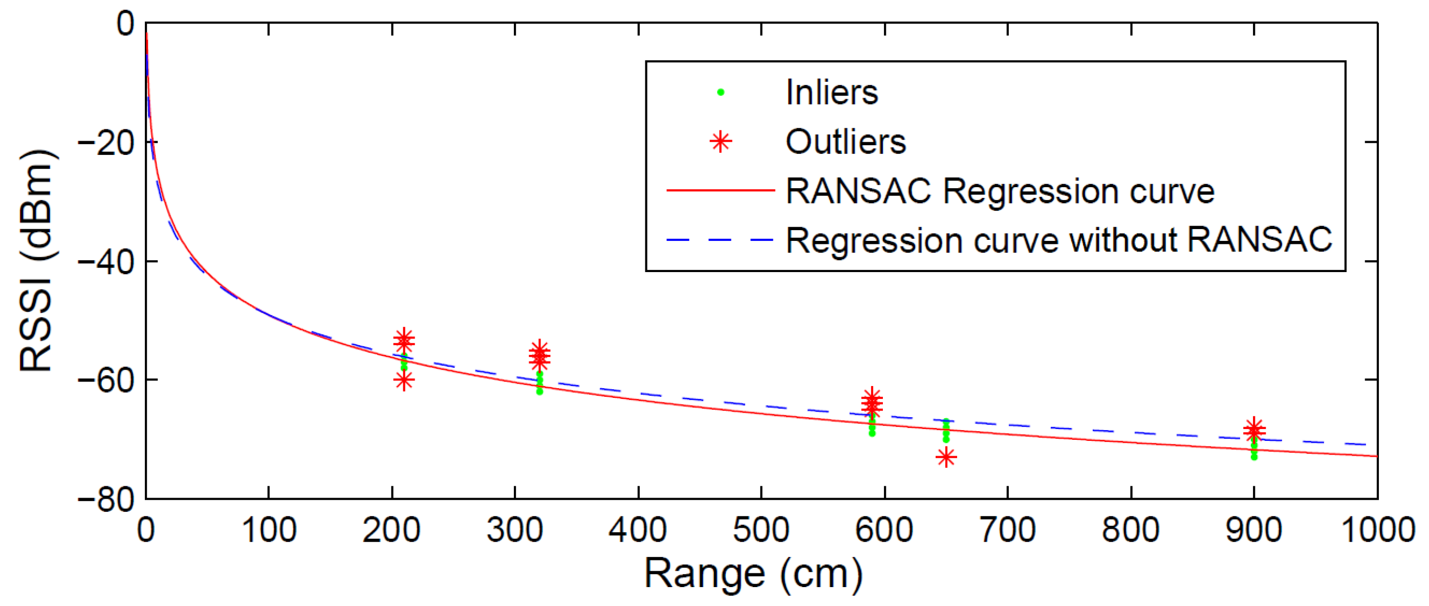
Figure 5 shows the model obtained with and without using RANSAC in an experiment performed in the UBILOC testbed. The figure shows 200 RSSI measurements taken by one static node from 5 anchor nodes. Although the RSSI measurements from each node showed low variability, the model fitting error can be high when considering all the measurements. The model obtained without RANSAC using all measurements was a = 9.51 and b = 5.34 , see Figure 5 in dashed line. The mean fitting error was 2.23 dBm. The outliers detected with the RANSAC algorithm are represented with asterisks. The model obtained with RANSAC using only inliers measurements—shown in solid line—yielded a = 10.302 and b = 1.678 , with a mean fitting error of 0.49 dBm. The differences between both models can be noticed in Figure 5 .
This method is computationally efficient and can be implemented by COTS WSN nodes. Each anchor node needs measurements from only two anchor nodes to on-line train its RSSI-range model. Of course, the model trained with few measurements will have lower accuracy that those trained with higher number of measurements. This method trains the RSSI-range model using measurements interchanged between anchor nodes. Hence, the trained model will capture the RSSI-range behavior at few discrete locations in the environment but, will not be able to capture the influence of the local surroundings of the moving target. This is the main advantage of the on-line training using target-anchor RSSI measurements, which is described in the next section.

5. On-Line Training Using Target-Anchor RSSI Measurements

In this method, anchor nodes are equipped with additional sensors that enable obtaining updated estimates of the target location. Each anchor node knows its own location and uses the estimation of the current target location to continuously adapt its own RSSI-range model. The resulting trained models are adapted to the local environments of the emitter (target) and receiver (anchor node). In this method each anchor node is assumed equipped with a camera and endowed with image processing and perception functions capable of estimating the current target location. Cameras have high energy consumption. Hence, in our method the cameras are only used to train the RSSI-range model and, not to perform target localization and tracking as e.g., reference [20], which would involve high energy consumption. The method includes mechanisms in which cameras are turned on to analyze the accuracy of the current trained RSSI-range model and update it if necessary. After that, the cameras are turned off to save energy.

5.1. Target-Anchor RSSI-Range Model Fitting

Let R S S I i , k be the RSSI measured by anchor node i from the packets it receives from the target. First we assume that each anchor node knows the updated location of the target. This will be relaxed in the next subsection. Assuming that each anchor node knows its location, anchor node i can collect a set of measurements ( R S S I i , k , d i , k ), where d i , k is the distance between the node i and the current target location. The objective is to dynamically obtain a RSSI-range model for anchor node i adapted to the local environment of the target at time k. This RSSI-range model can be approximated as linear: the anchor node i trains a RSSI-range model that is valid only in the proximity of the target current location. Locally the logarithm can be well approximated by a linear model, which reduces burden and simplifies its statistical-based analysis and filtering. In order to cope with the target motion, models are trained only with the M most recent pairs collected. Low values of M are typically selected. If the target moves, high M can involve RSSI measurements with different target local environments.
Hence, in this method a simple linear RSSI-range model for node i ( R S S I i , k = a i d i , k + b i ) (see Appendix A) is efficiently fit using Least Squares with measurement pairs ( R S S I i , k , d i , k ):
a i = k R S S I i , k d i , k R S S I i ¯ k d i , k k ( d i , k ) 2 d i ¯ k d i , k ,
b i = R S S I i ¯ ( a i d i ¯ ) ,
where R S S I i ¯ and d i ¯ stand for the mean of R S S I i , k and of d i , k .
The operation of the RSSI-range training is depicted in the diagram shown in Figure 6. The target starts periodically broadcasting RegrRequest packets. If anchor node i receives a RegrRequest packet, it measures its R S S I i and computes the range to the target d i , k . Hence, anchor node i obtains a measurement pair ( R S S I i , d i , k ) from each packet it receives from the target. If anchor node i has sufficient measurements, it can fit its RSSI-range model using Eqautions (4) and (5).
Only the M more recent measurements are used for model training. As anchor node i gathers more measurements it recalculates a i and b i enabling dynamic adaptation to the changing environment and reducing the size of the training pair set.

5.2. RSSI-Range Model Update

Section 5.1 assumed that the actual location of the target is known by all anchor nodes. Of course, this is not the case and nodes should estimate the target location. This technique uses estimates of the target location obtained from the cameras adopting a simple Maximum Likelihood (ML) approach that computes the location of the target that best matches with the observations gathered by the different cameras. The method used is summarized below.
Each sensor node gathers one image and applies image processing techniques to segment the target in the image. Let p i , k i m be the location (in pixels) of the center of the region where the target at time k has been segmented in the image from camera i. Assuming the camera pin-hole model is known, from p i , k i m it is easy to compute p i , k c , the location of the target on the scenario measured by camera i expressed in the reference frame local of camera i. Using T i , the transformation matrix from the reference frame of camera i w.r.t. a common reference frame, p i , k c can be transformed to p i , k s , which represents the location of the target measured by camera i in a common reference frame of the scenario. It is assumed that p i , k s contains errors that can be modeled as Gaussian statistically independent noise with zero mean noise and covariance matrix C o v i , k . Thus, the ML technique estimates the location of the center of the target as a Gaussian distribution with mean P k and covariance C o v k as follows [21]:
P k = ( i = 1 N C o v i 1 ) i = 1 N ( p i , k s C o v i , k 1 ) ,
C o v k = 1 / ( i = 1 N C o v i , k 1 )
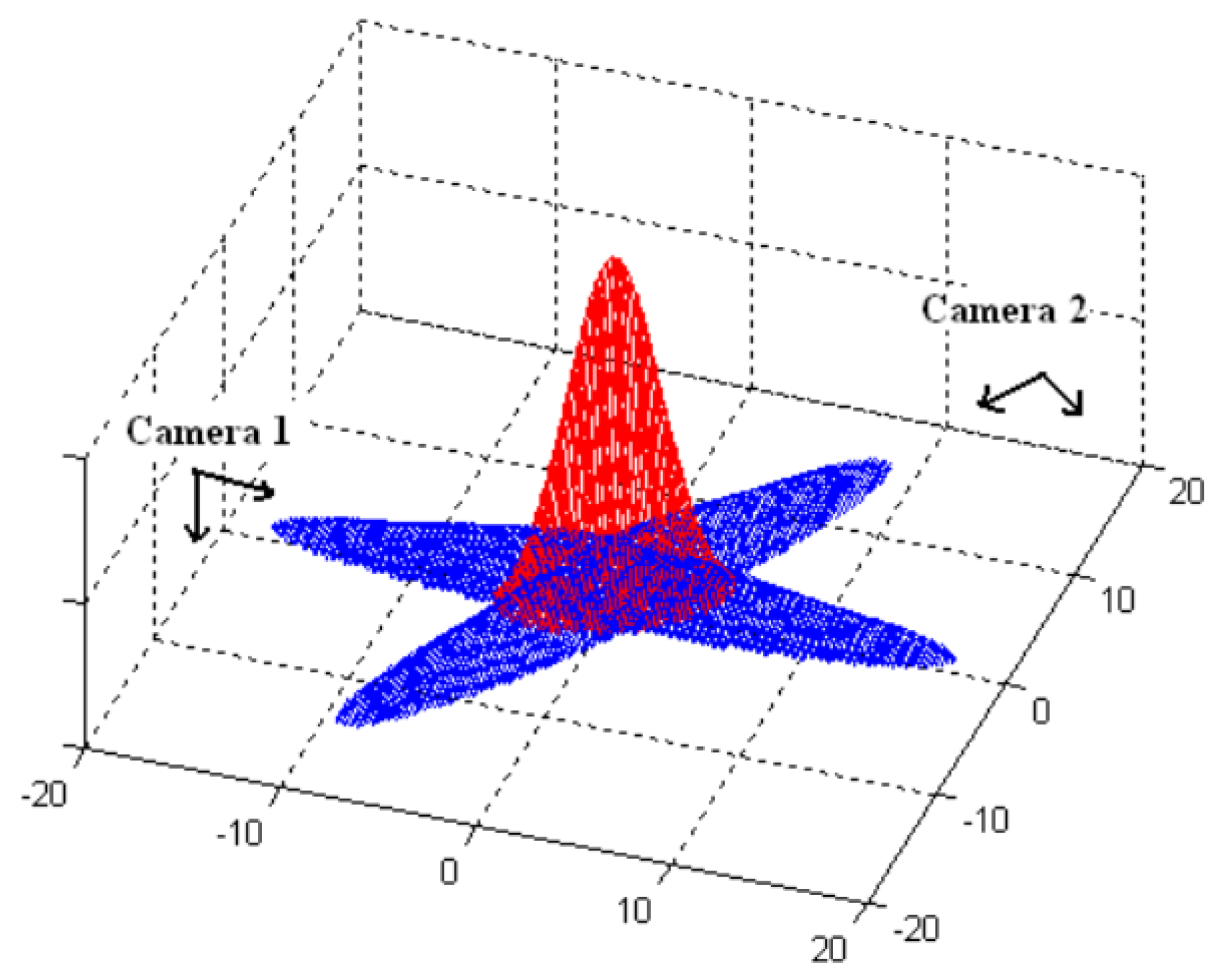
Each sensor node i broadcasts its values p i , k s and C o v i , k and combines them with those received from other nodes using Equations (6) and (7). Figure 7 shows an example of the ML technique with two cameras. The distributions of p i , k s for Camera1 and Camera2 are in blue color. For both cases the values of C o v i , k along the camera axes were assigned high to reflect the high uncertainty in the depth reconstruction when computing p i , k c . The resulting probabilities of the target location distribution ( P k ), in red color, are significantly higher, which denotes an increment in location accuracy. For more details on the method, please refer to reference [21].
The camera measurements are used only for RSSI-range model training. Each anchor node that is tracking a target periodically performs RSSI-range model update. During RSSI-range model update each node analyzes the accuracy of its RSSI-range model and updates it if its accuracy is found unsuitable. The operation is as follows. The target periodically transmits a RSSIRangeModelUpdate packet. In the experiments this frequency was 0.33 Hz. When an anchor node i—located at L i —receives it, it turns on its camera, gathers images and estimates the target location P k . The error of its RSSI-range model can be computed comparing the distance to the target estimated using camera measurements and the distance predicted by its RSSI-range model d i , k :
e i , k = ( R S S I i , k b i ) a i P k L i
The RMS error in the most recent N measurements is:
E i = 1 N k = 1 M e i , k 2
E i can be used to estimate the validity of the RSSI-range model. If E i < T H , the RSSI-range model of anchor node i is considered valid: it is not updated and the cameras are turned off. Otherwise, the RSSI-range model is considered invalid and should be computed using new ( R S S I i , k , d i , k ) pairs with Equations (4) and (5). After model training, the cameras are turned off. T H is the bound in the admissible error in the RSSI-range model and depends on the accuracy requirements of the application. Low values of T H originate frequent RSSI-range model update, which improves model accuracy but involves gathering more camera measurements and hence, higher energy consumption. High values of T H involve lower frequency in RSSI-range model update and hence, lower energy consumption. In preliminary experiments T H = 0.35 m 2 was found a good trade-off between model accuracy and energy consumption and it was adopted in the experiments shown in this paper.
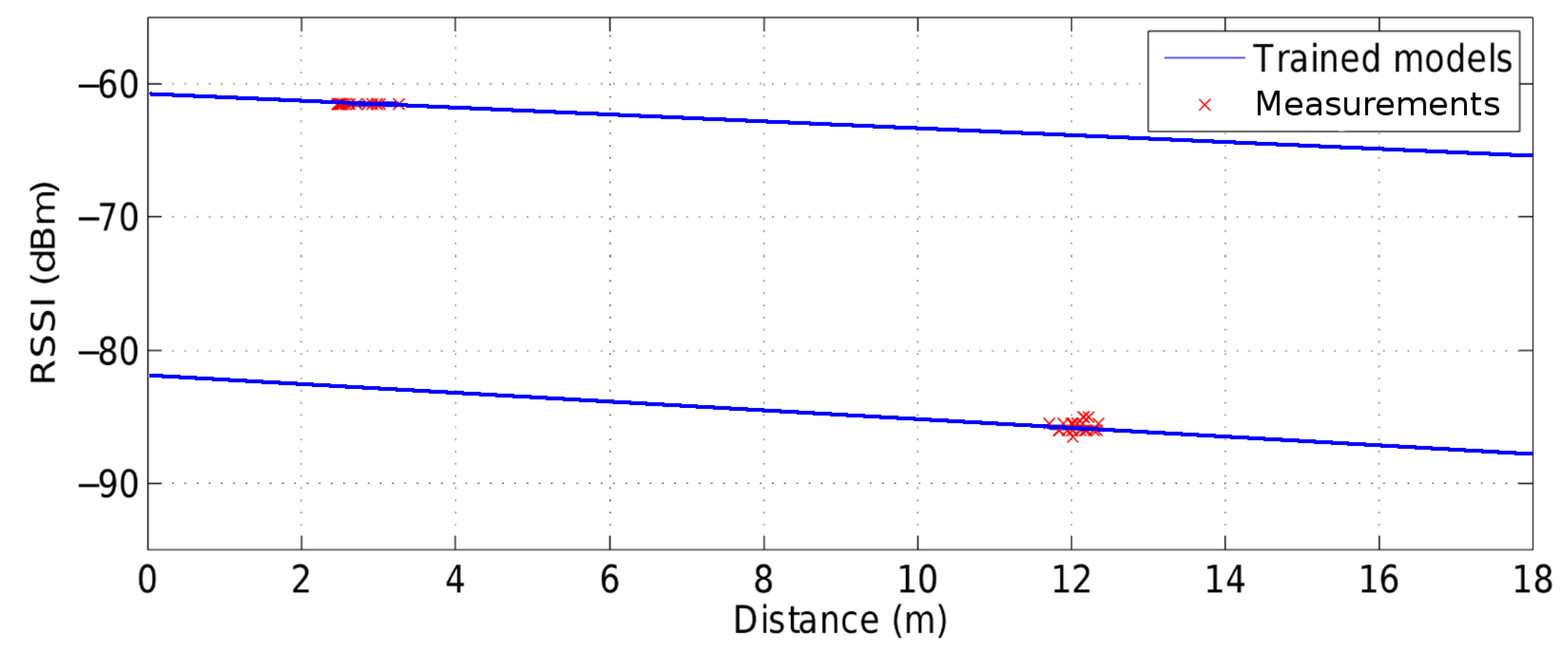
Figure 8 shows two trained RSSI-range models for anchor node i computed by the presented method when the target is at two different locations along the target path in one experiment performed in the UBILOC Testbed. The improvements in accuracy and fitting error over the default RSSI-range model in Figure 3 are evident. In this method the RSSI-range models are specific for each anchor node and trained to be accurate for the local surroundings of the target and, hence they are significantly more accurate than the default model.
It can be noticed in Figure 8 that, as expected, very few outliers were found when fitting the RSSI-range model. This result is consistent: the RSSI-range model is fitted to the local surroundings of the emitter and receiver, which can be considered static for all the M measurements used in the ( R S S I i , k , d i , k ) pairs.
It should be noticed that the inaccuracies in the estimation of P k can affect as perturbations in the RSSI-range model training. The proposed method includes a mechanism to specifically consider these errors. It is a statistical-based supervisor that estimates the variance of the error of the trained RSSI-range model. It operates as follows. Assume that d i , k = d i , k + u i , where d i , k is the distance from anchor node i to the target location P k estimated with the cameras, d i , k is the actual distance and u i is the error in the estimation of d i , k , which is highly related to the error in the estimation of the target position using camera measurements. Assume that R S S I i , k = a i d i , k + b i is the exact RSSI-range model and that the measured RSSI is R S S I i , k = R S S I i , k + v i , where v i is the RSSI measurement error. The training method uses pairs {( R S S I i , k , d i , k )} to fit the model R S S I i , k = a i d i , k + b i + v i . It is easy to check that the following expression holds:
R S S I i , k = a i ( d i , k + u i ) + b i + v i = R S S I i , k + a i u i + v i
In virtue of the Central Limite Theorem, u i and v i are assumed Gaussian White noises with zero means and variances σ u i 2 and σ v i 2 . Hence, the variance of the error of the trained RSSI-range model is:
σ t m , i 2 = a i 2 σ u i 2 + σ v i 2
Hence, it is very efficient to compute σ t m , i 2 . It depends on: σ v i 2 ; a i , the slope of its RSSI-range model; and σ u i 2 , the variance of the error in the estimation of d i , k , which can be easily computed from C o v k , the covariance of the error in the target location estimated with camera measurements. Trained RSSI-range models with higher a i are more sensitive to target location errors. Cases where 1 / a i = 0 are approximated by 1 / a i = ϵ and b i is recomputed using Equation (5) with the new a i .
The proposed method includes an efficient mechanism to evaluate the effect of estimation errors in the trained RSSI-range model. If σ t m , i 2 is higher than the variance of the default RSSI-range model, it means that the trained model is too noisy and it is considered invalid. In these cases, the default RSSI-model is preferred instead. As a result, badly trained RSSI-range models can be easily detected and, in those cases the default RSSI-range model is employed instead.
The presented technique allows obtaining RSSI-range models with accuracies similar to cameras but with very low energy consumption. Besides, it is endowed with mechanisms to self-detect and correct model training errors.

6. Experimental Section

In this section, the presented on-line RSSI-range modeling techniques are evaluated in real experiments. Both methods were inserted in the target localization and tracking scheme depicted in Figure 2 and experimented in the UBILOC Testbed. The Localization & tracking module in Figure 2, which estimated the target position using RSSI measurements, was implemented by a Kalman Filter (KF). A standard Kalman Filter was implemented. The only difference was that the observation model employed was not constant: it used the RSSI-range model trained on-line (during target tracking) by the two presented methods. Kalman Filters have been widely-employed in RSSI-based localization and tracking. For brevity, they are not presented in this paper.

6.1. The UBILOC Testbed

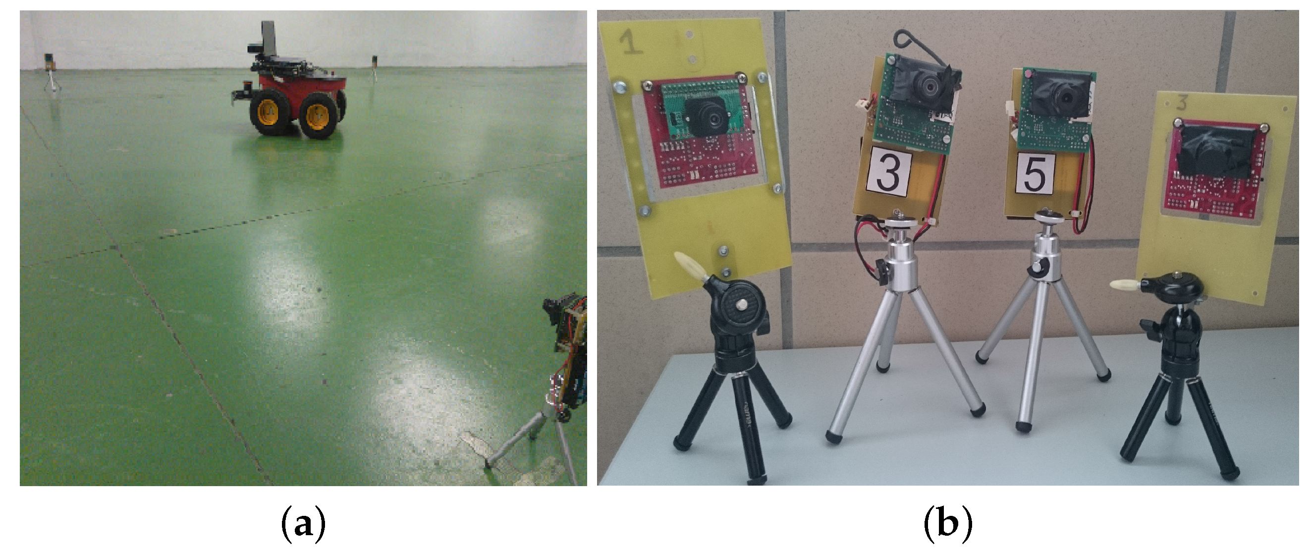
The Ubiquitous Localization Testbed (UBILOC) is a tool designed for experimenting localization and tracking techniques in ubiquitous computing systems, see Figure 9a. It emulates a typical office smart environment scenario and is deployed in a room of more than 500 m 2 in the basement of the School of Engineering of Seville. UBILOC was developed on top of the CONET Integrated Testbed [22,23], and inherits from it its main characteristics.
UBILOC includes sensors and systems widely used in localization and tracking in ubiquitous computing systems. It includes a WSN with static and mobile nodes. The mobile nodes are used as tags to be mounted on the targets to be localized and tracked. The static WSN nodes are deployed at 21 predefined locations hanging at 1.7 m height from the floor. It also includes a Wireless Camera Network (WCN). Each node of the WCN is composed by a CMUcam3 camera module [24] connected to a TelosB WSN node, see Figure 9b. CMUcam3 camera modules are endowed with embedded programmable image processing capabilities. Each CMUcam3 module captures RGB images and applies simple image processing methods. The results of the local image processing methods executed at each camera are transmitted to the TelosB node using a simple bidirectional protocol.
UBILOC also includes a set of mobile robots that are used as targets to be localized and tracked in the experiments. They enable high repeatability in localization and tracking experiments. Each robot is equipped with one 2D laser range finder and one Microsoft Kinect and an IEEE 802.11 Wireless bridge. Each robot is capable of accurately computing its own location and orientation using the Adaptive Monte Carlo Localization algorithm (AMCL) [25]. These location estimations are taken as the ground truth for evaluating target localization and tracking techniques in indoor experiments.

6.2. Proof of Concept

This section illustrates with a simple example the operation of the on-line target-anchor RSSI-range model training. The operation of the inter-anchor RSSI-range model technique is rather simple and it is not presented.
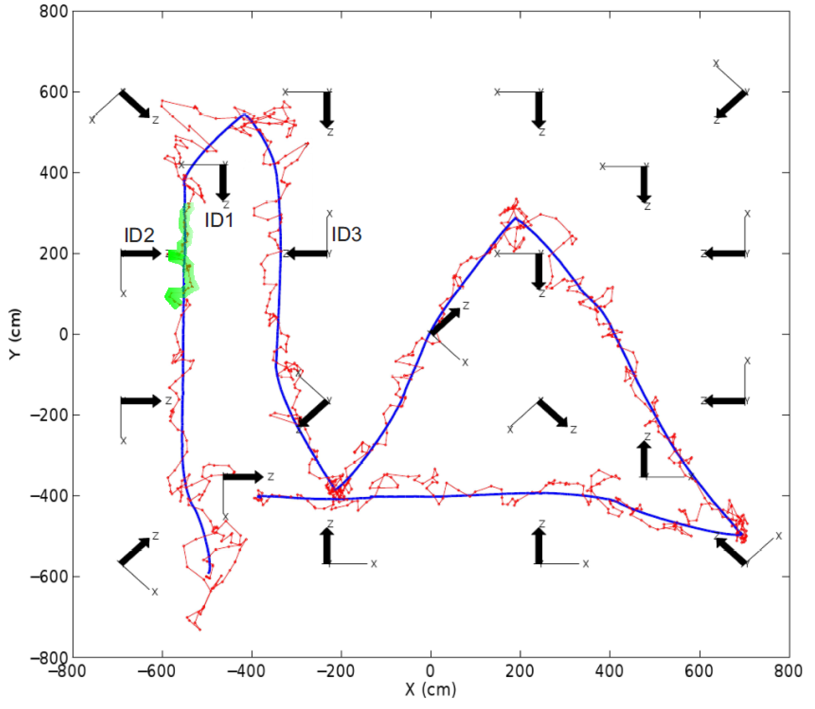
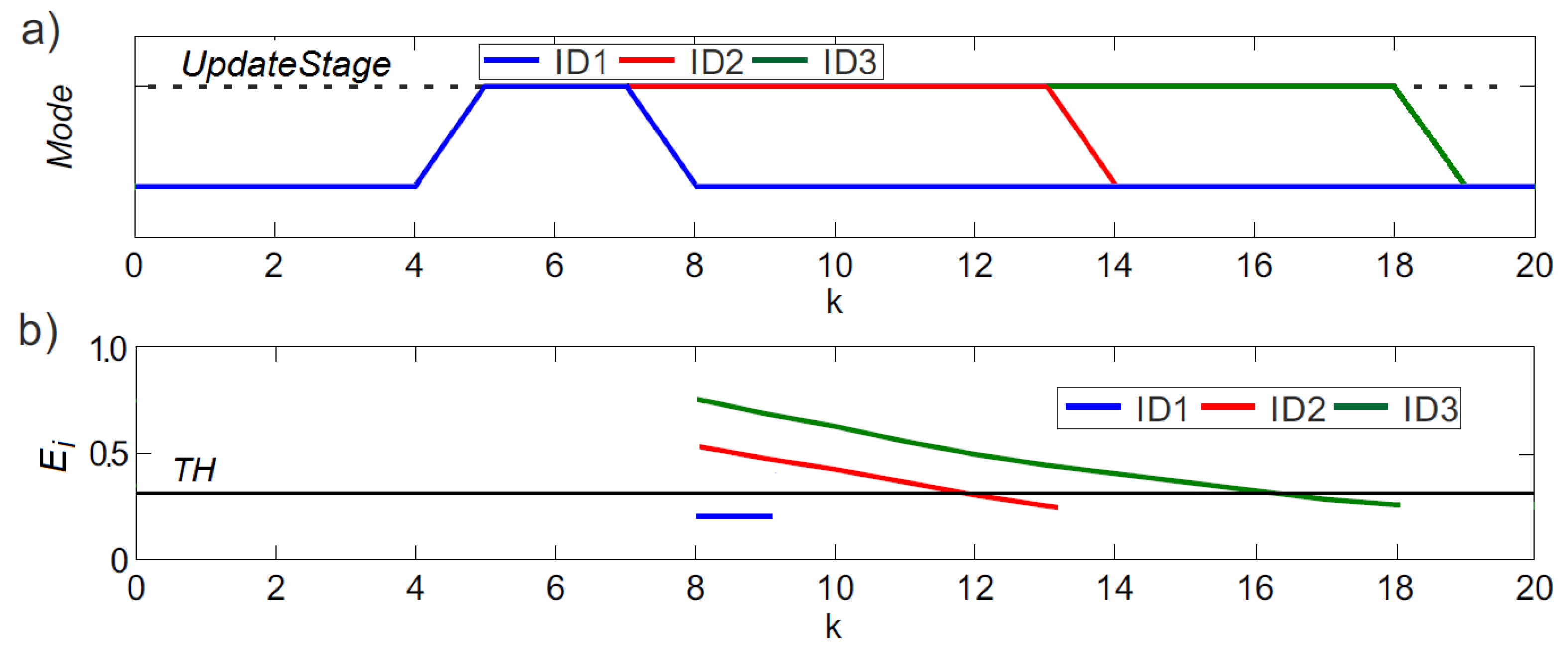
Figure 10 shows the result of a target localization and tracking experiment performed with the scheme in Figure 2 using the target-anchor RSSI-range model training method. The ground truth robot location is represented in blue and the estimated target location is in red. The camera local frames are also shown. Figure 10 shows in green the path followed by the robot between t = 550 s and t = 570 s. At t = 550 s anchor nodes ID1, ID2 and ID3 had their cameras off. This time is taken as k = 0 in Figure 11, which shows in a simplified way the operation of the target-anchor RSSI-range model training between k = 0 and k = 20. Figure 11a shows whether each of the involved anchor node is at its RSSI-range model update stage—high value—or not—low value. Figure 11b shows E i , the RMS error of the target-anchor RSSI-range model of each node along time. T H is also shown in Figure 11b.
Nodes ID1, ID2 and ID3 updated their RSSI-range model at t = 540 s. At time t = 574 s—i.e., k = 4—they received a RSSI Range Model Update packet from the target and started their RSSI-range model update stage. Each node turned on its camera, gathered visual measurements, used these measurements to estimate the target location and, with them computed E i , the RMS error of its RSSI-range model. If E i < T H the model for node i is considered valid: it finishes its RSSI-range model update stage and turns its camera off. This is the case of ID1, E i = 0.31 as shown in Figure 11b. ID1 finishes its RSSI-range model update stage and turns off its camera. Between k = 0 and k = 8, the cameras of nodes ID1, ID2 and ID3 are kept inactive. They cannot compute E i and it is not represented in Figure 11b.
If E i > T H the model for node i is considered invalid: it should update its RSSI-range model. This is the case of anchor nodes ID2 and ID3. With each new target location estimate, each of these nodes generated a new pair ( R S S I i , k , d i , k ) and used the M most recent pairs to train its RSSI-range model using Equations (4) and (5). Every time the RSSI-range model of node i is updated, the new E i is computed to evaluate the accuracy of the new model. Nodes ID2 and ID3 kept gathering visual measurements and updating their RSSI-model until they satisfied E i < T H . At that time the updated model was considered valid: the node finished its RSSI-range model update stage and turned its camera off. In the example in Figure 11 the RMS error of the RSSI-range model of ID3 was higher than that of ID2. ID2 needed to update the pair set ( R S S I i , k , d i , k ) with few measurements to compute an updated RSSI-range model that satisfied E i < T H . On the other hand, E i for node ID3 was higher and required more measurements. At k = 17 its trained RSSI-range model achieved E i < T H , ID3 finished its RSSI-range model update stage and turned its camera off .
In the presented target-anchor RSSI-range model training technique the cameras are active only while gathering measurements that are used for the regression of the RSSI-range model, which represents a low percentage of the time in the experiment. During the rest of the time the cameras are kept inactive saving energy.

6.3. Evaluation and Comparison

Both presented on-line RSSI-range modeling methods were employed in the scheme depicted in Figure 2 and evaluated in target localization and tracking experiments. The method using inter-anchor measurements was implemented as described Section 4. From now on it will be called M1. The method using target-anchor measurements was implemented as described Section 5. It is called M2.
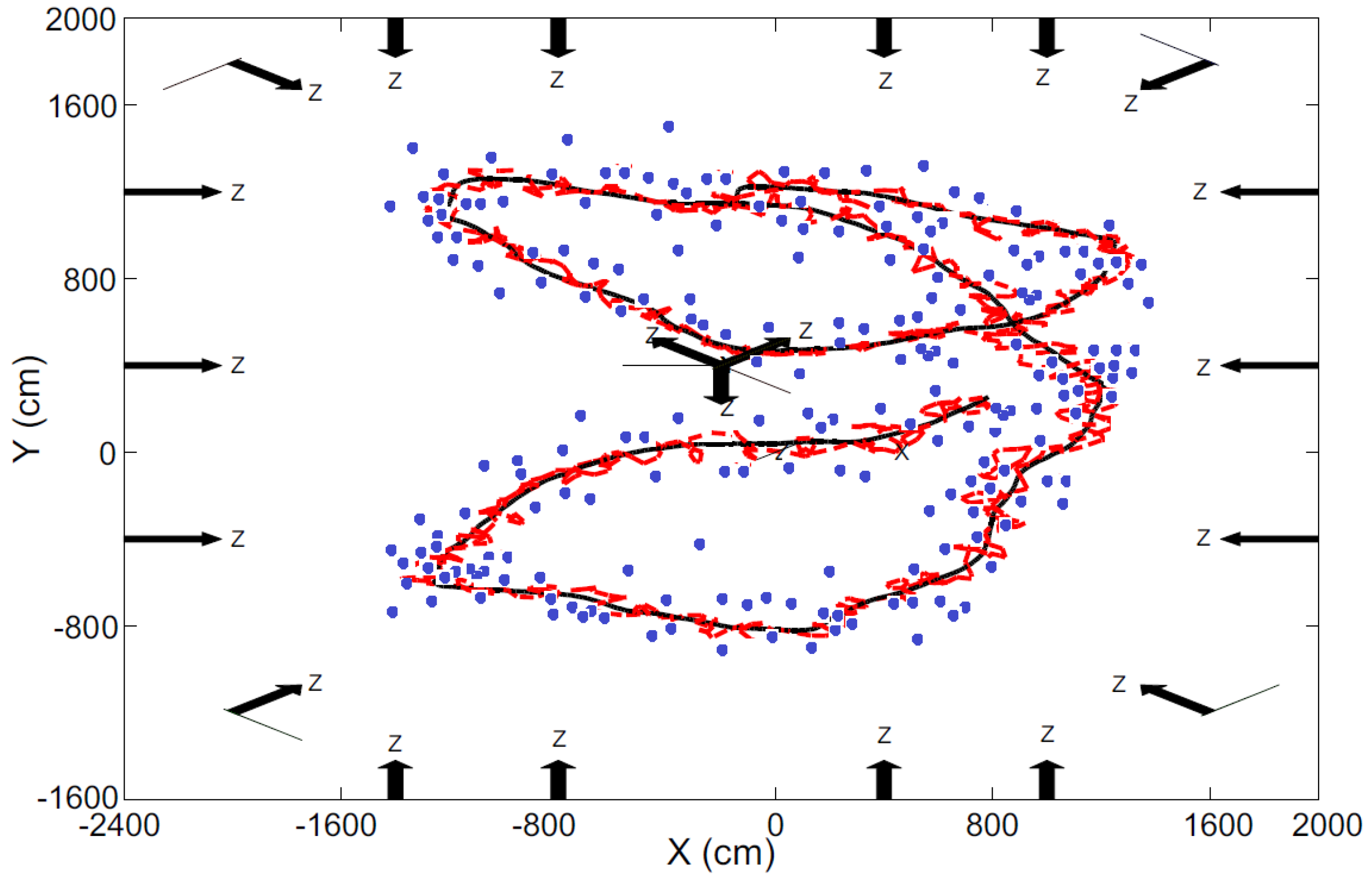
Consider the scenario shown in Figure 12, where 21 camera-nodes were deployed hanging from the ceiling (3 m height). The optical axis of all the cameras are also shown. The roll angle of all the cameras were zero. The target was a robot, which motion was controlled using the Player/Stage random walk functionality, in which it is given pseudo-random velocity commands. Figure 12 shows in black the trajectory actually described by the robot. The target location estimated using the tracking scheme in Figure 2 using M1 and M2 are represented respectively with dashed red lines and blue points. In this experiment M1 achieved an average localization error of 1.83 m and, M2, of 0.47 m.
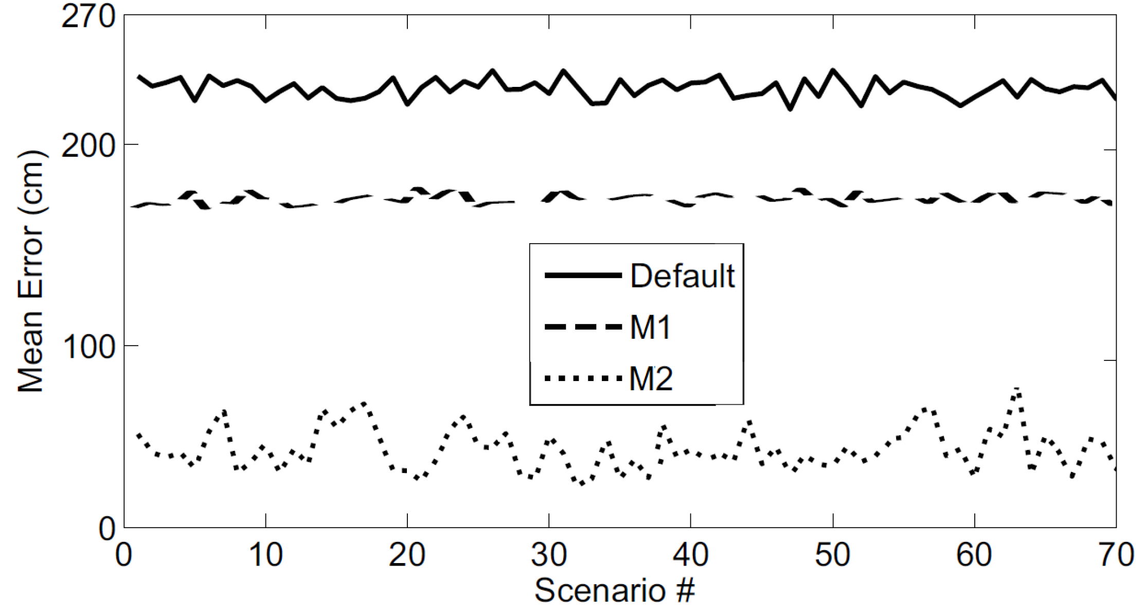
The accuracy of the presented on-line RSSI-range model training techniques was evaluated in a set of experiments with 70 random settings and robot trajectories. The camera nodes were deployed on the floor randomly using a uniform distribution in the range of the room size. The camera roll and pith angles of all the cameras were zero and the yaw angles were selected such that the optical axes pointed at the center of the room. We performed the experiments, logged all RSSI measurements and off-line processed the logs with the scheme in Figure 2 using three different approaches: the default RSSI-range model, method M1 and method M2. Figure 13 compares the mean localization error obtained using the three approaches.
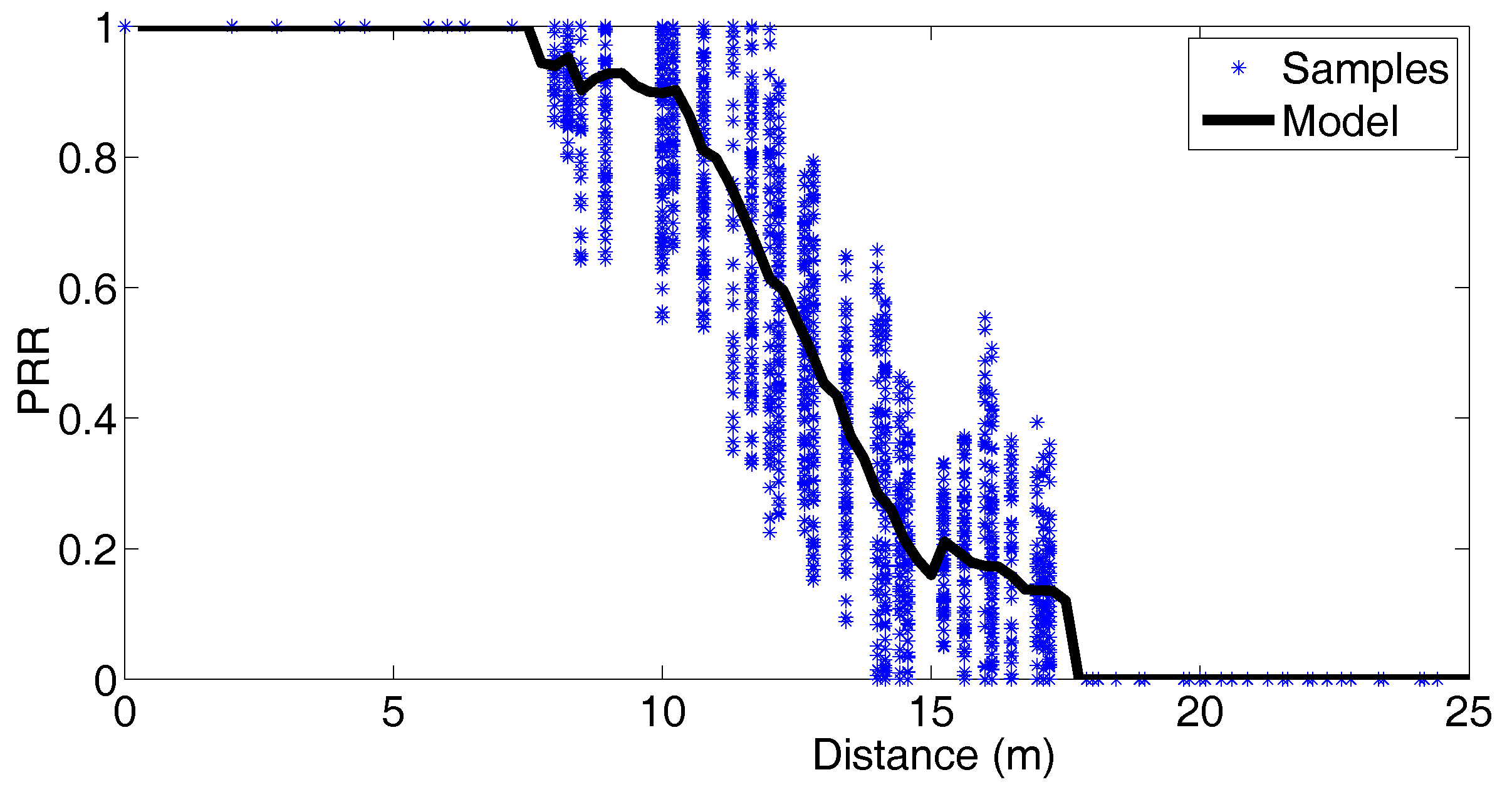
In average with M1 the target localization and tracking scheme had a localization error 18% lower than when using the default RSSI-range model. Also, with M2 the localization error was 77% lower than that of the scheme that uses the default model. The target-anchor RSSI-range modeling provides very accurate models. The experiments were performed assuming realistic conditions. For instance, Figure 14 shows the Packet Reception Rate (PRR) measured experimentally during the experiments.
Figure 15 shows the cumulate target localization errors obtained in the three cases: default, M1 and M2. M2 had significantly higher accuracy: the mean error was 53 cm and the error was lower than 97 cm in 80% of the samples. Errors were significantly higher in M1 and also in the default model.
M2 provides accurate models because it estimates target location with cameras and trains the RSSI-range model dynamically considering the local surroundings of the target and of the anchor node. Besides, it includes self-corrective tools that improve robustness against camera errors. Table 1 summarizes the performance of the target localization and tracking scheme with the default model, the models resulting from methods M1 and M2. In M2 the cameras were active during an average of 11.5% of the total duration of the experiment. Considering the energy consumption of TelosB WSN nodes and CMUcam3 modules, which can be found in their data-sheets, the energy consumed by M2 was 140.75 mW, 61% higher than in case of using the default model and method of M1, which did not use cameras. M2 obtains localization and tracking errors similar to vision-based methods but requires having the cameras active only during a small fraction of the experiment duration and hence, has significantly lower energy consumption than tracking systems based solely on cameras.

6.4. Discussion

M, the number of measurement pairs used in RSSI-range model regression, is critical both for M1 and for M2. On one hand, higher values of M reduce inaccuracies in model fitting. On the other hand, using older measurements reduces their capability to adapt to the changes in the scenario, particularly in M2, which uses target-anchor measurements and the target is usually in motion.
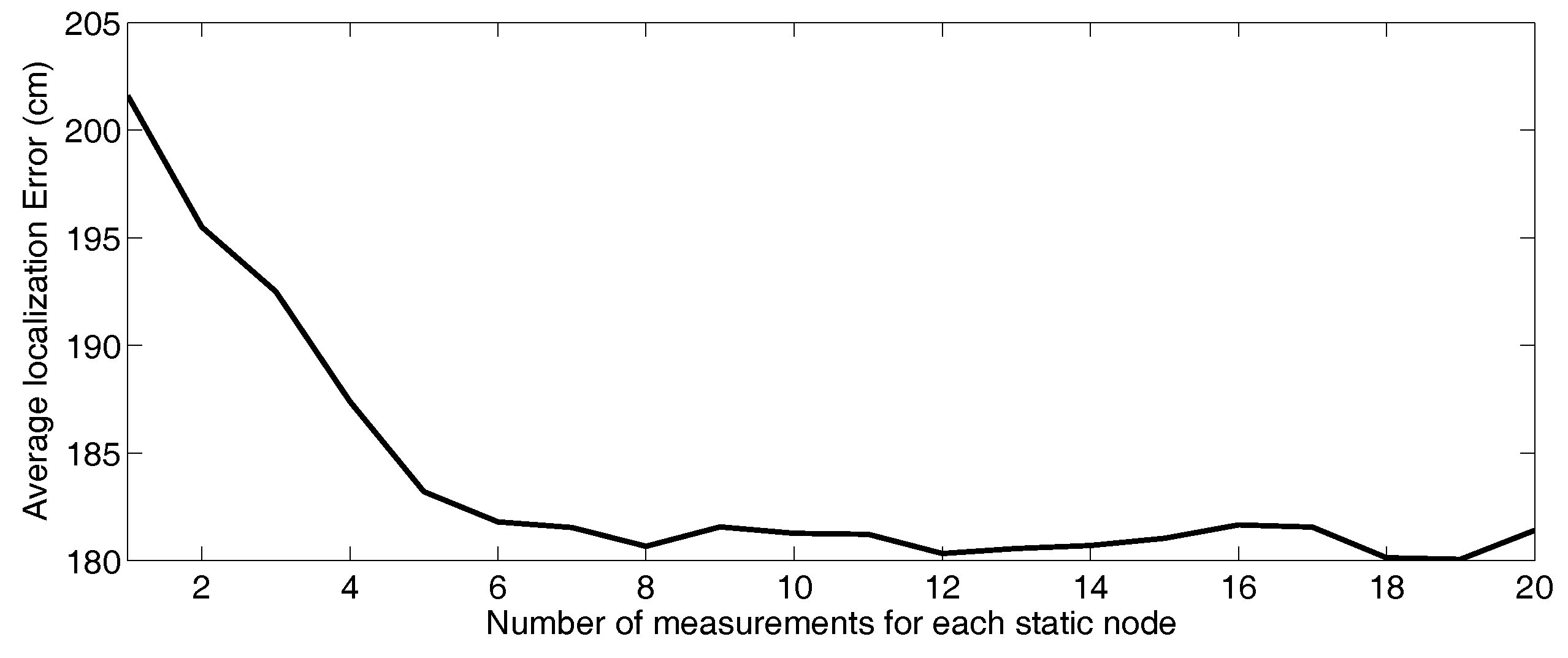
Figure 16 shows the average target tracking error in the above experiments when using M1 with different values of M. In M1 the models trained with fewer measurement pairs were less accurate than those fitted with higher M. With less than 3 measurements from each anchor node, the trained RSSI-range model obtained errors that are similar to those when using the default RSSI-range model. It was necessary to select at least M = 5 to exploit the benefits of on-line fitting. However, the target tracking error did not decrease when using M > 7. Taking higher M involved higher computational burden but did not increase the accuracy of the RSSI-range model.
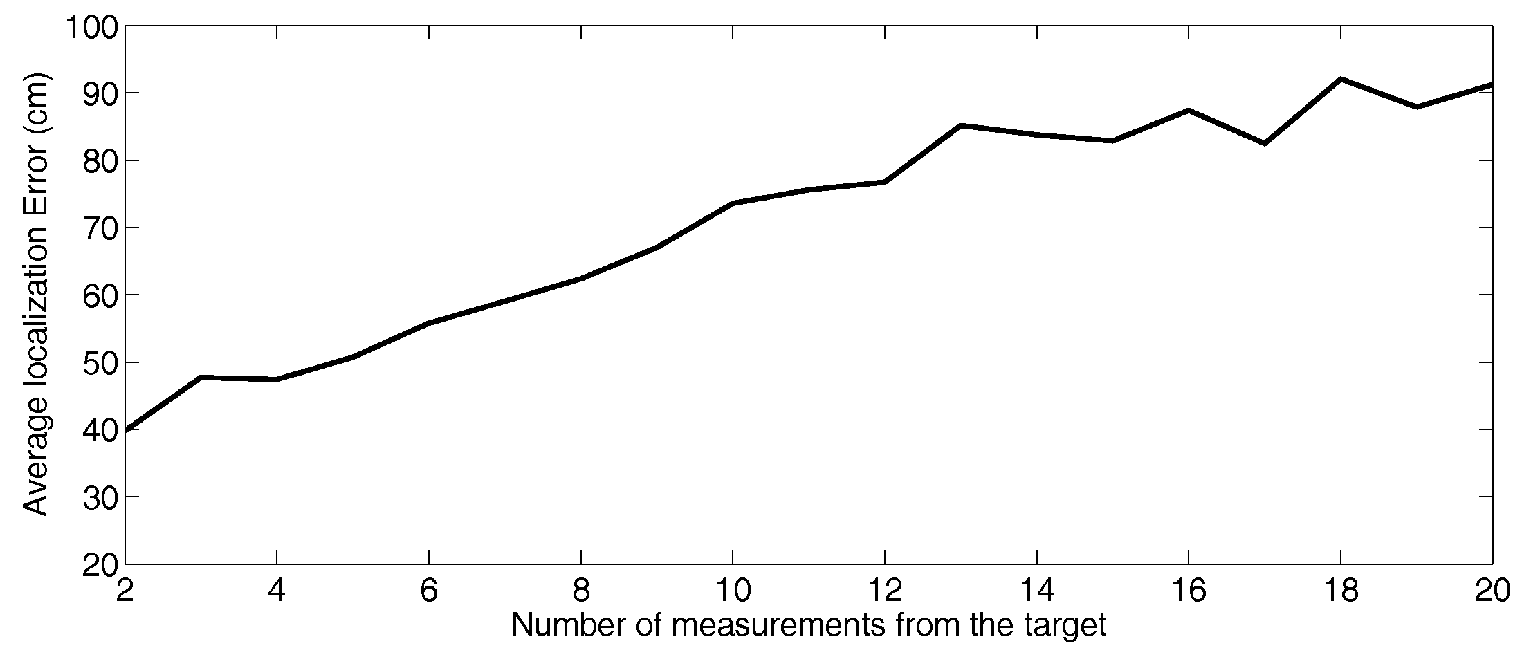
Figure 17 shows the average target tracking error when using M2 with different values of M. In M2 linear RSSI-range models enable accurate fitting even when using very low number of measurement pairs. With higher M the RSSI-range models were less accurate since the target was in motion and with a higher number of measurement pairs the model was not fitted to the surroundings of the target but to a wider area, loosing accuracy.
In the following, the complexity (number of operations) of M1 and M2 are estimated. Assume that in M1 the measurements of K anchor nodes are used in the training of the RSSI-range model of each anchor node. M is the number of measurement pairs employed in the regression. Also, the RANSAC algorithm performs I iterations and F is the fraction of samples taken for the RANSAC initial fitting. The complexity of M1 without outlier rejection is O ( 2 K M ) . The complexity of outlier rejection in M1 increases proportionally to the number of RANSAC iterations I. The complexity of M1 with RANSAC is O ( 2 I F K M ) . The complexity of scheme M2—without including the number of operations to compute P k —is O ( M ) .
We take typical values for the above parameters in the experiments performed in UBILOC: K = 5, M = 7, I = 4 and F = 0.2 for M1 and, M = 4 for M2. Method M1 without RANSAC requires N O M 1 = 73 operations and M1 with RANSAC requires N O M 1 R = 537 operations. The use of RANSAC for outlier rejection requires significant burden and the improvement in accuracy can be interesting in some applications. Method M2 requires only N O M 2 = 11 operations. M2 is very efficient but requires accurate target location estimates obtained with other sensors such as cameras. M2 is very interesting if anchor nodes are equipped with cameras.

7. Conclusions

RSSI is the most widely used measurement for localization and tracking in ubiquitous computing systems. RSSI can be measured by most radio modules used in COTS WSN nodes without incurring in extra delay, computational or energy consumption costs. However, RSSI measurements are highly affected by perturbations originated by interactions of the radio signal with the environment, which significantly disturb the accuracy of RSSI-based localization techniques.
Most range-based localization methods use a general RSSI-range model that assumes free-space radio propagation and considers these perturbations as noise. However, this noise is correlated and does not satisfy the hypotheses assumed by these techniques, involving high localization errors. Some techniques adopt a training-based approach in which they off-line learn the RSSI-range characteristics of the environment in a prior training phase. However, the training phase is a long off-line time-consuming process, which must be repeated if there have been changes in the environment, lacking adaptability.
This paper deals with methods in which each anchor node on-line learns its RSSI-range model adapted to the particularities of its environment and uses its trained model for localization and tracking. In the presented methods the training stage is performed during the localization stage, enabling adaptability to scenario changes. Two techniques are presented. The first method (M1) uses the information of the location of the anchor nodes to dynamically adapt the RSSI-range model. The second methods (M2) uses the target location estimated by anchor nodes equipped with cameras to on-line adapt the RSSI-range model. The presented methods operate in real-time and only require a few measurements to compute updated RSSI-range models.
The presented techniques have been integrated in a target localization and tracking scheme based on Kalman Filter and evaluated in experiments performed in the UBILOC Testbed. In average with M1 had a localization error 18% lower than when using the default RSSI-range model. M1 does not require camera measurements and had the same energy consumption as the default case. The localization error in M2 was 77% lower than when using the default model. In M2 the cameras were active during 11.5% of the total duration of the experiment, involving an energy consumption 61% higher than in M1 or in the default case. Hence, M2 obtains localization and tracking errors similar to vision-based methods but requires having the cameras active only during a small fraction of time, involving high energy savings w.r.t. systems based solely on cameras.

Acknowledgments

This work was developed mainly in the context of EU Project MULTIDRONE (H2020-ICT-2016-2017/H2020-ICT-2016-1). Partial funding was obtained from EU Project AEROARMS Ref. H2020-ICT-2014-1-644271 and the AEROMAIN project funded by the Spanish R&D plan (DPI2014-59383-C2-1-R). José Ramiro Martínez-de Dios acknowledges EU Project AEROBI funded under contract H2020-ICT-2015-1-687384.

Author Contributions

José Ramiro Martínez-de Dios was the main designer of the scheme and algorithms that led to this paper, coordinated the experiments and elaborated the major part of the manuscript. Anibal Ollero provided suggestions and corrections during the preparation of the manuscript. Francisco José Fernández and Carolina Regoli participated in the implementation and evaluation of the methods.

Conflicts of Interest

The authors declare no conflict of interest.

Appendix A. Derivation of RSSI-Models

In the basic radio free-space propagation model the following expression holds:
R S S I ( D ) = P 0 ( D 0 ) 10 n p log ( D / D 0 ) ,
where R S S I ( D ) is the value of RSSI in dBm at distance D, P 0 ( D 0 ) is the strength of the transmitter in dBm at a reference distance D 0 , n p is the path loss exponent. Mathematically, Equation (A1) can be expressed as:
R S S I ( D ) = 10 n p log ( D ) + P 0 ( D 0 ) + 10 n p log ( D 0 )
n p depends on the environment. In a model training approach D 0 and P 0 ( D 0 ) are treated as unknowns that are fitted during training. In a model training problem, Equation (A2) can be expressed as:
R S S I ( D ) = a log ( D ) + b ,
where a = 10 n p and b = P 0 ( D 0 ) + 10 n p log ( D 0 ) .
This RSSI-range model reflects the numerical relations between RSSI and range. Although it is simple for efficient RSSI-range model training, it is actually derived as a simplification of physical radio free-space propagation model as explained below. The linear RSSI-range model used in Section 5 is also an experimental RSSI-range model which objective is to numerically relate the values of RSSI and range. This RSSI-range model is computed continuously and hence it is enough to compute a simple model valid for the surroundings of the target.

References

  1. Baccour, N.; Koubaa, A.; Mottola, L.; Zuniga, M.A.; Youssef, H.; Boano, C.A.; Alves, M. Radio link quality estimation in wireless sensor networks: A survey. ACM Trans. Sens. Netw. 2012, 8, 34:1–34:33. [Google Scholar] [CrossRef] [Green Version]
  2. Wang, X.; Bischoff, O.; Laur, R.; Paul, S. Localization in Wireless ad-hoc Sensor Networks using multilateration with RSSI for logistic applications. Procedia Chem. 2009, 1, 461–464. [Google Scholar] [CrossRef]
  3. Savvides, A.; Han, C.; Strivastava, M. Dynamic fine-grained localization in ad-hoc Networks of Sensors. In Proceedings of the International Conference on Mobile Computing and Networking, Rome, Italy, 16–21 July 2001; pp. 166–179. [Google Scholar]
  4. Benkic, K.; Malajner, M.; Planinsic, P.; Cucej, Z. Using RSSI value for distance estimation in wireless sensor networks based on ZigBee. In Proceedings of the 15th International Conference on Systems, Signals and Image Processing (IWSSIP’2008), Bratislava, Slovak Republic, 25–28 June 2008; pp. 303–306. [Google Scholar]
  5. Zhang, J.; Zhang, L. Research on distance measurement based on RSSI of ZigBee. In Proceedings of the International Colloquium on Computing, Communication, Control, and Management (CCCM’2009), Sanya, China, 8–9 August 2009; Volume 3, pp. 210–212. [Google Scholar]
  6. Liu, C.; Wu, K.; He, T. Sensor localization with ring overlapping based on comparison of received signal strength indicator. In Proceedings of the IEEE International Conference on Mobile Ad-hoc and Sensor Systems, Fort Lauderdale, FL, USA, 25–27 October 2004; pp. 516–518. [Google Scholar]
  7. He, T.; Huang, C.; Blum, B.M.; Stankovic, J.A.; Abdelzaher, T. Range-free localization schemes for large scale Sensor Networks. In Proceedings of the International Conference on Mobile Computing and Networking, San Diego, CA, USA, 14–19 September 2003; pp. 81–95. [Google Scholar]
  8. Bahl, P.; Padmanabhan, V.N. RADAR: An in-building RF-based user location and tracking system. In Proceedings of the Annual Joint Conference of the IEEE Computer and Communications Societies (INFOCOM’2000), Tel Aviv, Israel, 26–30 March 2000; pp. 775–784. [Google Scholar]
  9. Smailagic, A.; Kogan, D. Location sensing and privacy in a context-aware computing environment. IEEE Wirel. Commun. 2002, 9, 10–17. [Google Scholar] [CrossRef]
  10. Youssef, M.A.; Agrawala, A.; Shankar, A.U.; Noh, S.H. A Probabilistic Clustering-Based Indoor Location Determination System; Technical Reports; UMIACS: College Park, MD, USA, 2002. [Google Scholar]
  11. Roos, T.; Myllymäki, P.; Tirri, H.; Misikangas, P.; Sievänen, J. A probabilistic approach to WLAN user location estimation. Int. J. Wirel. Inf. Netw. 2002, 9, 155–164. [Google Scholar] [CrossRef]
  12. Hassan-Ali, M.; Pahlavan, K. Site-specific wideband and narrowband modeling of indoor radio channel using ray-tracing. In Proceedings of the Personal, Indoor and Mobile Radio Communications (PIMRC’98), Boston, MA, USA, 8–11 September 1998; pp. 65–68. [Google Scholar]
  13. Hassan-Ali, M.; Pahlavan, K. A new statistical model for site-specific indoor radio propagation prediction based on geometric optics and geometric probability. IEEE Trans. Wirel. Commun. 2002, 1, 112–124. [Google Scholar] [CrossRef]
  14. Awad, A.; Frunzke, T.; Dressler, F. Adaptive distance estimation and localization in WSN using RSSI measures. In Proceedings of the Conference Digital System Design Architectures, Methods and Tools (DSD’2007), Lubeck, Germany, 29–31 August 2007; pp. 471–478. [Google Scholar]
  15. Vanheel, F.; Verhaevert, J.; Laermans, E.; Moerman, I.; Demeester, P. Automated linear regression tools improve rssi wsn localization in multipath indoor environment. EURASIP J. Wirel. Commun. Netw. 2011, 2011, 1–27. [Google Scholar] [CrossRef] [Green Version]
  16. Mihaylova, L.; Angelova, D.; Bull, D.R.; Canagarajah, N. Localization of Mobile Nodes in Wireless Networks with Correlated in Time Measurement Noise. IEEE Trans. Mob. Comput. 2011, 10, 44–53. [Google Scholar] [CrossRef] [Green Version]
  17. Patwari, N.; Hero, A.O.; Perkins, M.; Correal, N.S.; O’dea, R.J. Relative location estimation in wireless sensor networks. IEEE Trans. Sig. Process. 2003, 51, 2137–2148. [Google Scholar] [CrossRef]
  18. Itoh, K.-I.; Watanabe, S.; Shih, J.-S.; Sato, T. Performance of handoff algorithm based on distance and RSSI measurements. IEEE Trans. Veh. Technol. 2002, 51, 1460–1468. [Google Scholar] [CrossRef]
  19. Fischler, M.A.; Bolles, R.C. Random sample consensus: a paradigm for model fitting with applications to image analysis and automated cartography. Commun. ACM 1981, 24, 381–395. [Google Scholar] [CrossRef]
  20. De San Bernabé, A.; Martínez-de Dios, J.R.; Ollero, A. Efficient cluster-based tracking mechanisms for camera-based wireless sensor networks. IEEE Trans. Mob. Comput. 2015, 14, 1820–1832. [Google Scholar] [CrossRef]
  21. Sánchez-Matamoros, J.M.; Martínez-de Dios, J.R.; Ollero, A. Cooperative localization and tracking with a camera-based WSN. In Proceedings of the International Conference on Mechatronics (ICM2009), Malaga, Spain, 14–17 April 2009; pp. 1–6. [Google Scholar]
  22. Jiménez-González, A.; Martínez-de Dios, J.R.; Ollero, A. An integrated testbed for heterogeneous mobile robots and other cooperating objects. In Proceedings of the IEEE/RSJ International Conference on Intelligent Robots and Systems, Taipei, Taiwan, 18–22 October 2010. [Google Scholar]
  23. Jiménez-González, A.; Martínez-de Dios, J.R.; Ollero, A. An integrated testbed for cooperative perception with heterogeneous mobile and static sensors. Sensors 2011, 11, 11516–11543. [Google Scholar] [CrossRef] [PubMed]
  24. Rowe, A. CMUcam3 Datasheet. 2012. Available online: http://www.cmucam.org/ (accessed on 9 August 2017).
  25. Fox, D.; Burgard, W.; Dellaert, F.; Thrun, S. Monte carlo localization: Efficient position estimation for mobile robots. In Proceedings of the AAAI/IAAI, Orlando, FL, USA, 18–22 July 1999; pp. 343–349. [Google Scholar]
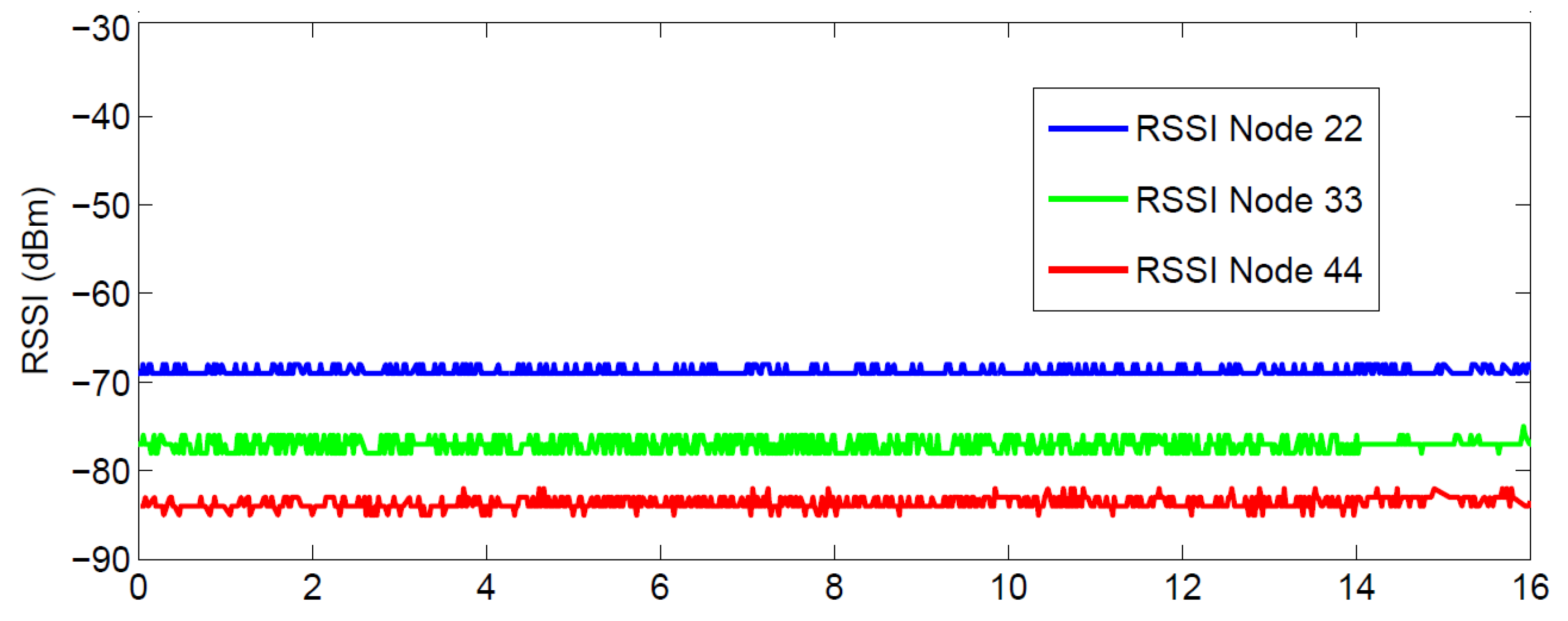
Figure 1. Result of RSSI variability experiments between three different anchor WSN nodes and the same receiver.
Jsan 06 00015 g001
Figure 2. (a) General target localization and tracking scheme with on-line trained RSSI-range models; (b) Geometrical setting of the scenario.
Jsan 06 00015 g002
Figure 3. RSSI-range model experimentally obtained in the UBILOC Testbed.
Jsan 06 00015 g003
Figure 4. Operations and communications between anchor node i and the rest of anchor nodes for inter-anchor RSSI-range model training.
Jsan 06 00015 g004
Figure 5. Experimental RSSI-range models obtained with and without RANSAC.
Jsan 06 00015 g005
Figure 6. Operations and communications between anchor node i and the target in target-anchor RSSI-range model training.
Jsan 06 00015 g006
Figure 7. Simple example of the ML technique.
Jsan 06 00015 g007
Figure 8. Trained RSSI-range linear models obtained in an experiment in the UBILOC Testbed using target-anchor RSSI measurements.
Jsan 06 00015 g008
Figure 9. (a) Picture of the UBILOC Testbed during an experiment; (b) Nodes of the WCN: each node is composed of a CMUcam3 module and a TelosB WSN node.
Jsan 06 00015 g009
Figure 10. Result of an experiment performed with the scheme in Figure 2 using target-anchor RSSI-range model training: ground truth in solid (blue) and estimated location (in red).
Jsan 06 00015 g010
Figure 11. Performance of nodes ID1, ID2 and ID3 in the experiment shown in Figure 9 between second t = 550 s (k = 0) and second t = 570 s (k = 20): (a) mode of anchor nodes ID1, ID2 and ID3; (b) values of E i of each node along time.
Jsan 06 00015 g011
Figure 12. Result of a target localization and tracking experiment performed in UBILOC: ground truth is the solid black line, the target location estimated using M1 and M2 are represented respectively with dashed red lines and blue points.
Jsan 06 00015 g012
Figure 13. The mean localization error obtained by the scheme in Figure 2 when using the three approaches: Default, M1 and M2 in 70 different experiments performed in UBILOC.
Jsan 06 00015 g013
Figure 14. Packet Reception Rate obtained experimentally in the described experiments.
Jsan 06 00015 g014
Figure 15. Cumulative target localization errors obtained by the scheme Figure 2 in the above experiments when using the default model, method M1 and method M2.
Jsan 06 00015 g015
Figure 16. Average tracking error in Figure 2 with M1 when using different number of measurement pairs.
Jsan 06 00015 g016
Figure 17. Average tracking error in Figure 2 with M2 when using different number of measurement pairs—M.
Jsan 06 00015 g017
Table 1. Performance when using the default model, and those resulting from methods M1 and M2.
DefaultM1M2
Average localization error (m)2.321.890.53
Average time cameras are active (% of the experiment time)0011.5%
Average sensor node energy consumption (mW)6666140.75